Design Hourly Volume Estimation at Freeway Nodes From Short-Term Traffic Counts

Abstract

This paper extends the concept of a design hourly volume (DHV) which is derived from the “nth hour” to a concept based on the nth highest saturated hour. To calculate this nth highest saturated hour at each ramp junction of a node, it is necessary to have permanent traffic counts (PTC) on all ramps and the main lanes. In practice, such counts are often not available. For such cases, the German Highway Capacity Manual proposes a method that enables the estimation of DHV through short-term traffic counts (STCs) and the extrapolation of the results using available PTC in the vicinity. This study examines how accurately the required nth highest saturated hour can be estimated with this method and similar concepts. Furthermore, we investigate to what extent the number and the location of the available PTC affect the accuracy of the estimation. Scenarios without PTC are also considered. The evaluation is based on a database with a total of 72 freeway nodes for which PTC data from three years (2017–2019) are processed. The results show that the estimation of the nth highest saturated hour with the method of the German Highway Capacity Manual works accurately, even if only one PTC is available on each inflowing approach. The results further indicate that STC are crucial to achieve accurate results when few PTCs are available. Acceptable results are also obtained by STC of one week, even without a projection at a PTC.

Estimating the design hourly volume (DHV) is an essential step when it comes to estimating the level of service (LOS) of traffic facilities. In both the Highway Capacity Manual (HCM) ( 1 ) and the German HCM (Handbuch für die Bemessung von Strassenverkehrsanlagen) ( 2 ), DHV is determined based on a concept for DHV estimation known as the nth hour, or the hour of the year with the nth highest traffic volume. This implies designing the traffic facility in such a way that it is only oversaturated in n−1 hours per year, with typical values for n ranging between 30 and 200 h per year. To calculate this nth hour precisely, it is necessary to have a permanent traffic count (PTC) at the corresponding traffic facility, since the traffic volume for all 8,760 h of the year must be known. If no PTC is available, the DHV can be alternatively estimated using short-term traffic counts (STCs). Appropriate methods are provided by the Federal Highway Administration’s (FHWA) Traffic Monitoring Guide (TMG) ( 3 ).

These methods refer exclusively to freeway segments with only one traffic stream. A method for the estimation of the DHV at nodes (freeway exits and interchanges on freeways) or ramp junctions (merging, diverging, and weaving segments) using STC (and its extrapolation using nearby PTC) is proposed by the German HCM.

At ramp junctions, determining the nth hour for each of the streams separately would lead to an inconsistent demand-situation since these volumes would most likely not occur at the same hour. Thus, an artificial demand-situation would be created, which did not occur in reality. Figure 1 illustrates this as an example for the 50th hour of a merging segment: the 50th hour of the traffic stream on the main lane upstream is measured at 5:00 p.m. in the afternoon peak hour (a), whereas the 50th highest traffic volume on the on-ramp occurs at 07:00 a.m. in the morning peak hour (b). The 50th hour of the main lane upstream corresponds to the 206th hour of the on-ramp (a), whereas the 50th hour of the on-ramp appears at the time of the 3768th hour of the main lane upstream (b). Calculating the LOS for each of these different hours (using the methods of the German HCM), leads to considerably different results: in the 50th hour on the main lane upstream, the result is LOS F, whereas in the 50th hour of the on-ramp, it results in LOS D. Considering the traffic volume downstream of the merging segment (c), the 50th hour of this total traffic volume results in the 45th hour on the main lane upstream and the 678th hour of the stream on the on-ramp, which results in LOS E. This example shows that the estimated LOS of a ramp junction can depend highly on the decision of which traffic stream is considered when determining the 50th hour or the DHV in general. This raises the question which of these approaches provides the most appropriate result for the design of traffic facilities.

Figure 1.

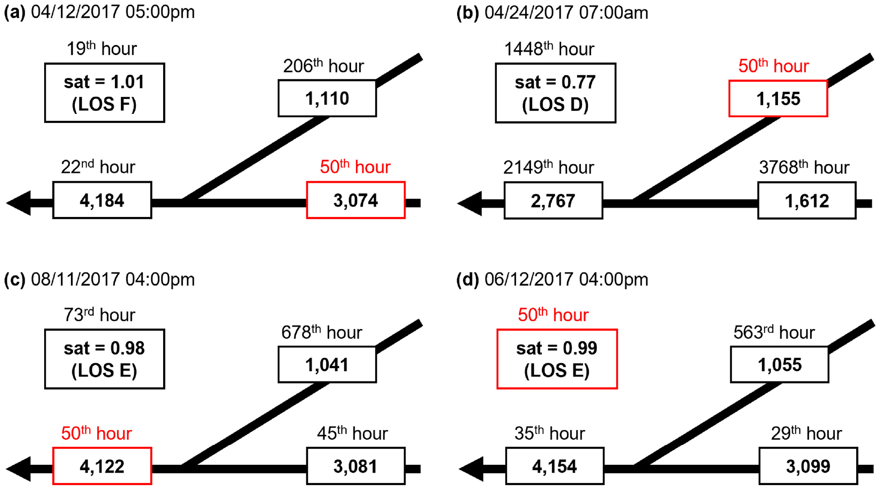
Saturation rate (sat), level of service (LOS), and traffic volume (vehicles per hour) of all streams in the 50th hour of the main lane upstream (a), the on-ramp (b), the main lane downstream (c), and the saturation rate (d).

The concept for DHV estimation of the nth hour requires that the traffic facility may be congested at a maximum of n−1 hours in the observed year. This implies that only n−1 hours of the year may have a LOS of E or worse, as this is the threshold of acceptable traffic stream quality according to the definition of the German HCM (analogous to the HCM). As LOS is a rather aggregated metric, it seems more appropriate to consider the metric from which the LOS is derived instead. According to the German HCM, LOS is derived from the saturation rate. For this reason, the DHV corresponds to the traffic volumes in the hour with the 50th highest saturation rate (d).

This paper examines how the nth highest saturated hour can be estimated by combining STC and PTC considering the topology of a node. For this purpose, we generalize the method proposed in the German HCM and analyze six concepts for DHV estimation at nodes. It is also examined how the number of available PTCs affects the accuracy of an estimation. To achieve this, five data availability scenarios are distinguished in which the numbers and locations of the available PTCs are varied. Scenarios with and without PTC are considered. The combinations of a concept for DHV estimation and a data availability scenario lead to DHV estimation scenarios. These DHV estimation scenarios are calculated and analyzed to investigate the accuracy of estimating the nth highest saturated hour based on STC and the extrapolation with PTC with the method proposed in the German HCM.

Literature Review

The procedure for estimating the DHV on basic freeway segments based on STC can be divided into two sub-steps: the extrapolation of the results of a STC to an annual average daily traffic (AADT) value, and the determination of the DHV from the AADT. In the following literature review, studies are considered that deal with these two sub-steps.

To estimate AADT from STC or short-period traffic counts (SPTC), the TMG ( 3 ) proposes the following method. First, group the available PTC stations into groups of road sections with similar temporal traffic variations, then determine average seasonal adjustment factors for each of these groups. The road section monitored with STC is assigned to one of the road section groups. The STC results are extrapolated to an AADT using the corresponding seasonal adjustment factor of the assigned road section group.

Gecchele et al. ( 4 ) and Gastaldi et al. ( 5 ) further develop this method in the sense that the grouping of the PTC is performed using a fuzzy C-means algorithm, and neural networks are used for the assignment of the monitored road section. The authors select 25 PTC stations of a rural road network to validate the presented method. These PTC are grouped and used to derive 775 sample SPTCs each covering one week. The study shows satisfactory results for the AADT estimates that could be obtained with SPTC of one week. It is found that the results depend on the period during which the SPTCs are carried out, assuming that socio-economic and land-use characteristics influence the temporal pattern of the local travel demand. The authors recommend incorporating these characteristics in future models ( 5 ).

Khan et al. ( 6 ) apply machine-learning approaches such as artificial neural networks and support vector regression to develop models for estimating AADT from STC. According to the authors, support vector regression is the most appropriate model, especially when incorporating hourly volume data and day-of-week and month-of-year as categorical features. It is found that including socio-economic factors into the model lowers the model performance. The authors conclude that the AADT of a location is primarily based on temporal traffic patterns like day-of-week or month-of-year.

Bagheri et al. ( 7 ) propose a method that improves the matching of STC to PTC or groups of PTC by including all historical counts collected for these sites in the model. The proposed two-pattern matching methods can significantly improve the performance of the TMG method ( 3 ). Ha ( 8 ) compares the TMG method with a similar method used in South Korea. The results show that it can be helpful to carry out two days of STC, one in each half of the year. Sharma et al. ( 9 ) investigate the reliability of daily truck traffic estimates from STC and Figliozzi et al. ( 10 ) the estimation of the AADT of non-motorized traffic.

Capparuccini et al. ( 11 ) compare three different methods for determining the DHV. The first method is determining the DHV manually from the peak hour of the design day during the week of STC. The remaining two methods estimate the DHV from the AADT by multiplying a K-factor, which represents the relative proportion of the DHV on the AADT. The methods differ in their approach to determining the K-factor. The performance of the methods is tested based on 74 PTCs. For each PTC, 10 weekly counts are simulated by extracting the traffic volumes of the corresponding week and estimating the DHV with each of the three methods. The estimated DHV are then compared with the actual DHV (30th hour), which are calculated based on all 8,760 hours of the year for the corresponding PTC. The simplest method of manually determining the DHV provides the best results. This result shows that the K-factor must be chosen very well to obtain accurate results.

Petković et al. ( 12 ) propose a model that also determines the DHV as a function of AADT but is considering the ratio of the daily volume of the design weekday to AADT and the ratio of the daily volume on Saturday to AADT. The model is developed using statistical analysis of 2016 PTC data and is then tested on the data of 2015 and 2017. The model provides accurate results with the advantage that classification of road sections based on the traffic flow characteristics is not required.

Liu and Sharma ( 13 ) investigate holiday peaking characteristics and the contributions of holiday travel to the yearly highest hourly volumes for rural highways in Alberta, Canada. Based on the analyzed data (PTC of 20 years), genetic algorithms are used to develop models for the prediction of DHV. The study demonstrates that models assisted by genetic algorithms are very robust and suitable for determining the DHV.

Concepts for DHV Estimation at Freeway Nodes: Combining PTC and STC

The literature review indicates that STC may be a suitable data source for determining the DHV when data from PTC are not available. However, the studies all refer to count stations on basic freeway segments. An equivalent concept for DHV estimation in the context of a node has not yet been investigated in detail. The German HCM ( 2 ) shows an example of how to combine PTC and STC using topological relationships of a freeway interchange: The example assumes that a cloverleaf interchange, as shown in Figure 2, has eight PTC, one for each inflow or outflow, and at least two STC for each ramp junction. Each PTC defines a specific demand-situation, which needs to be analyzed. In the following, these demand-situations are referred to as PTC demand-situations.

Figure 2.

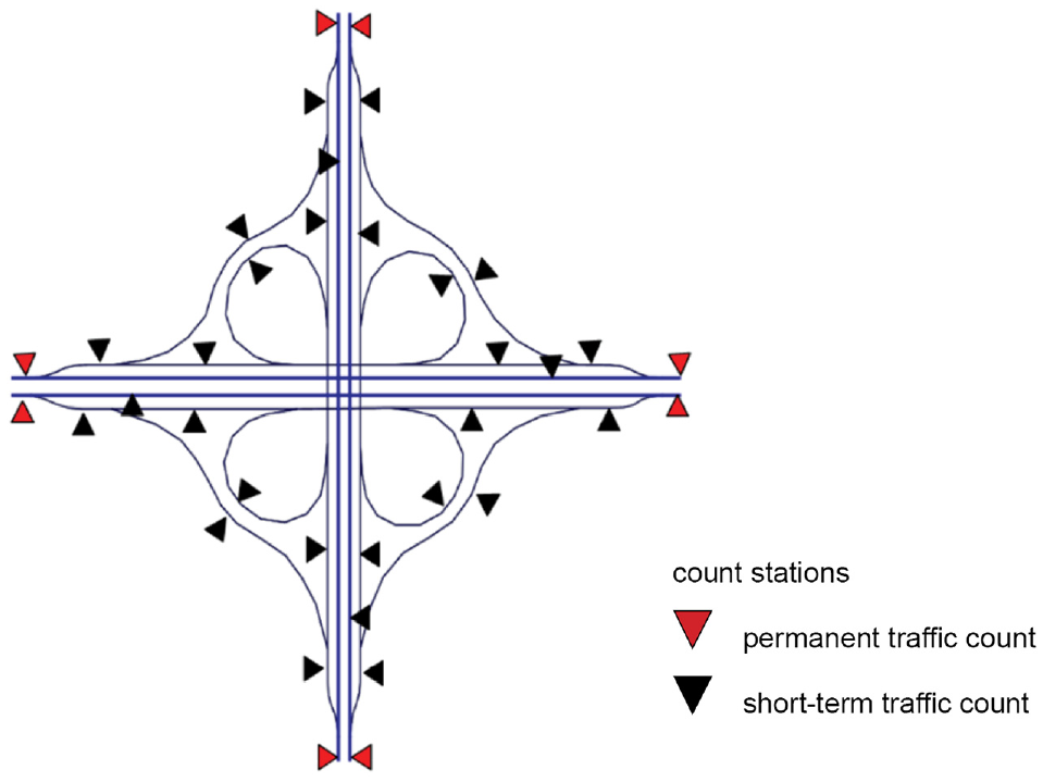
Count stations on a cloverleaf interchange based on an example in the German Highway Capacity Manual (2).

Each PTC demand-situation describes a temporary state with consistent traffic volumes at the entire interchange, such that inflow equals outflow. In the German HCM ( 2 ), these demand-situations are defined using the method “50th hour of the PTC”. For the example in Figure 2 this leads to eight demand-situations, which may occur on different weekdays and times of day. Considering the example merging segment in Figure 1, we can define three PTC demand-situations (a), (b), and (c), that is, one PTC demand-situation per PTC. Each PTC demand-situation has a different date and time, for example April 12 at 5:00 p.m. (a), April 24 at 7:00 a.m. (b), and September 8 at 4:00 p.m. (c).

STC are usually conducted at a different date. Therefore, the German HCM uses the hour of the day of the PTC demand-situation to derive a second demand-situation based on the STC (STC demand-situation). For the PTC demand-situation (a) in Figure 1, the STC demand-situation is 5:00 p.m. In the next step a matrix estimation method is applied using the PTC demand-situation as boundary conditions and the STC demand-situation as initial matrix to derive DHV for each count station.

This procedure is repeated for all eight PTC demand-situations of the cloverleaf interchange. After that, all eight demand-situations are evaluated. For each ramp junction, a separate saturation rate is estimated per demand-situation. The resulting saturation rate of a ramp junction is the worst case saturation rate of all demand-situations considered.

This approach can be generalized as follows. A concept for DHV estimation in the context of a node has four components:

• basic concept for DHV estimation for PTC, for example the 50th hour

• demand-situation(s) for the PTC (PTC demand-situation)

• demand-situation for the STC (STC demand-situation), which can depend on the PTC demand-situation

• data extrapolation procedure, for example matrix estimation

The basic concept for DHV estimation defines the traffic volumes of the PTC demand-situation. The combination of PTC demand-situation and STC demand-situation serves as input for the data extrapolation procedure. In this way, the PTC demand-situation defines boundary conditions for the extrapolation procedure and the STC demand-situation defines initial information of the traffic streams for all relations, that is, origin–destination flows at the node. Using matrix estimation as a data extrapolation procedure, we obtain the general procedure to calculate the DHV based on PTC and STC on freeway nodes:

1. Define all PTC demand-situations, including traffic volumes for all PTC, with reference to the basic concept for DHV estimation.

2. For each PTC demand-situation:

3.   b. For each STC demand-situation perform a matrix estimation with an initial matrix from the STC demand-situation and the boundary condition from the PTC demand-situation.

For our analysis, we define four concepts for DHV estimation for the DHV in the context of a freeway node (Table 1) with PTC. They are applied to the general procedure described above. Note: In this study, the 50th highest saturated hour is examined as a representative of the nth highest saturated hour.

1. 50th hour (STC: day hour): This is the concept used in German HCM described in the example above. This concept applies PTC demand-situations with consistent traffic flows at the entire interchange (inflow equals outflow).

2. 50th hour (STC: mPH or aPH): To analyze the influence of using a specific day hour for the STC demand-situation, which depends on the 50th hour of a PTC, we define a second concept by changing the way of deriving the STC demand-situation. Here the STC demand-situation does not depend on the day hour of the PTC demand-situation but is based on either the morning peak hour (mPH) or afternoon peak hour (aPH) of the STC considering the total traffic volume of all counting stations of the node. Which peak hour is chosen depends on whether the 50th hour occurs in the morning or in the afternoon. The PTC demand-situations are the same as in the concept “50th h (STC: day hour),” thus providing consistent traffic flows.

3. 30th–70th hour (STC: frequent day hour): This concept varies the method of DHV estimation at the PTC. Instead of the 50th hour, the mean traffic volumes of the 30th–70th hour are considered. To achieve consistent traffic flows at the node, each examined PTC demand-situation defines 41 hours of the year (calendar day and day hour). Traffic volumes at neighboring PTC stations are computed as the average of volume for these 41 time points. For the STC demand-situation this concept uses the most frequent day hour of all examined 41 hours.

4. 30th–70th h (STC: mPH+aPH): This concept also uses the 30th–70th hour for the DHV estimation at the PTC, but instead of considering one PTC demand-situation for each PTC, it only considers one PTC demand-situation with an average volume for each PTC station. This leads to a PTC demand-situation where traffic flows are not consistent. As STC demand-situation, the concept distinguishes two cases: one demand-situation for the morning peak hour of the STC considering all counting stations of the node and one demand-situation for the afternoon peak hour.

The STC demand-situation is consistent for all four concepts. If there is no PTC available, the German HCM suggests STC for a week, using the peak hour as DHV estimation for a single count station. To extend this approach to a node, we define two additional concepts covering only STC:

1. STC PH week (worst case): The concept defines one demand-situation per count station, which is derived from the weekly peak hour of the count station. For each ramp junction, the worst case is considered. Each demand-situation shows consistent traffic flows.

2. STC PH week (one demand-situation): This concept defines one demand-situation combining the peak hours of all count stations. This demand-situation has inconsistent traffic flows.

Furthermore, the number of PTCs and STCs can be varied, which leads to different data availability scenarios. They are defined and explained in the section “Data Availability Scenarios.”

Table 1.

Overview of the Six Concepts for Design Hourly Volume (DHV) Estimation and Their Attributes

Name of concept for DHV estimation	Basic concepts for DHV estimation for PTC	Number of DHV estimation scenarios	PTC demand-situation	STC demand-situation	Consistent traffic streams
50th hour (STC: day hour)	nth hour	Number of PTC stations × number of STC days	One for each PTC	Day hour of 50th hour	yes
50th hour (STC: mPH or aPH)	nth hour	Number of PTC stations × number of STC days	One for each PTC	Morning peak hour or afternoon peak hour, using 50th hour	yes
30th–70th hour (STC: frequent day hour)	Mean value for a range of hours around the nth hour	Number of PTC stations × number of STC days	One for each PTC	Most frequent day hour in set of 30th–70th hours	yes
30th–70th hour (STC: mPH+aPH)	Mean value for a range of hours around the nth hour	2 day times × number of STC days	One including all PTC	Morning peak hour and afternoon peak hour	no
STC PH week (worst case)	PH of week	Number of ramp junctions × number of weeks of year	-	One demand-situation per ramp junction, no matrix estimation necessary	yes
STC PH week (one demand-situation)	PH of week	1 × number of weeks of year	-	One demand-situation including peak hours of all ramp junctions	no

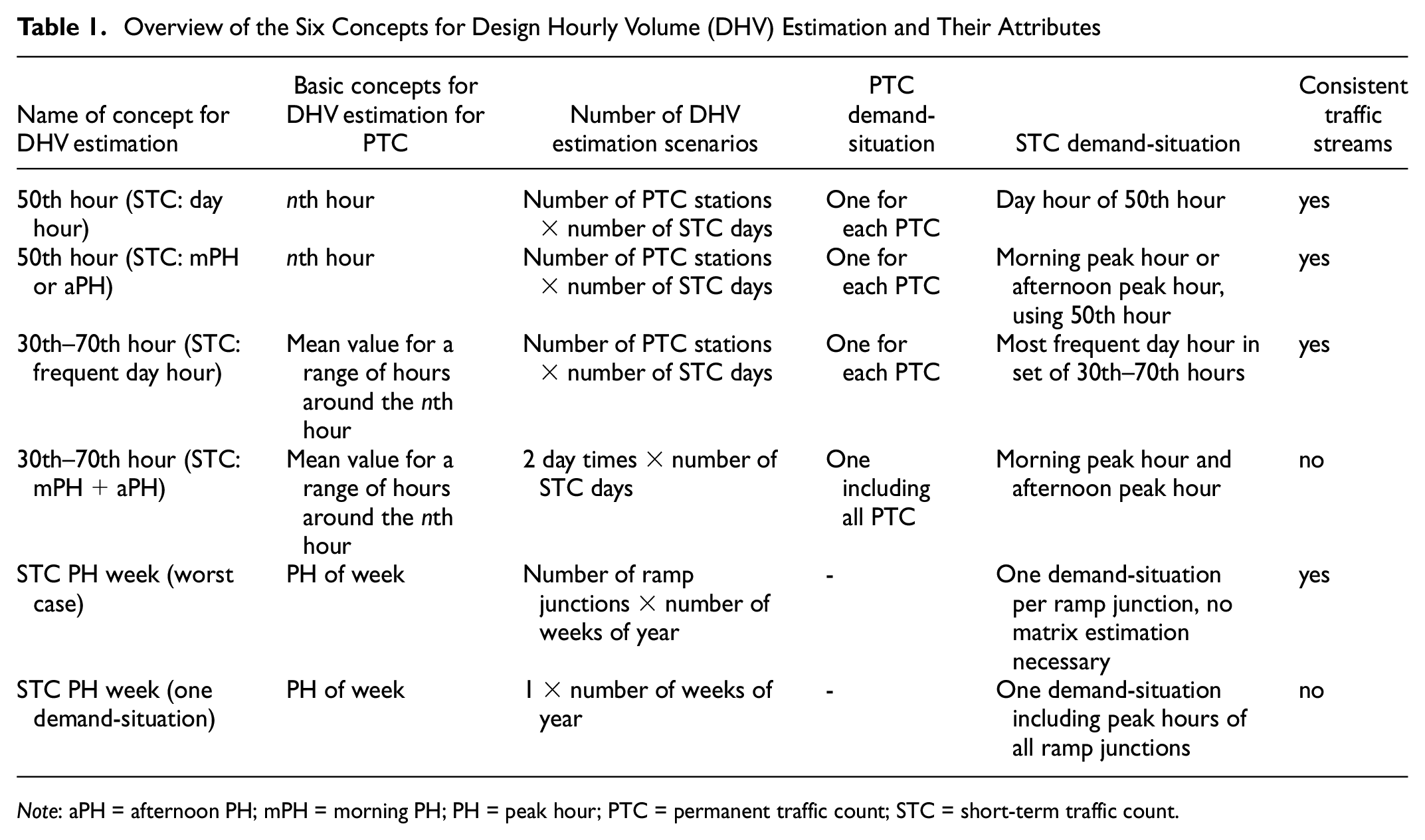
Note: aPH = afternoon PH; mPH = morning PH; PH = peak hour; PTC = permanent traffic count; STC = short-term traffic count.

Methodical Approach

The intention of this study is to investigate how accurately the nth highest saturated hour of a ramp junction can be determined using the method proposed by the German HCM, depending on the STC demand-situation and the number and location of the PTC stations.

For this purpose, a reference database is first created based on real-world PTC data from 2017, 2018, and 2019, which includes 72 nodes overall. The available traffic count data are expanded in such a way that the traffic volume is known for each main lane and ramp for all 8,760 h of the year. The German HCM evaluation procedures for the calculation of the saturation rate, as well as the proposed methods for DHV estimation based on STC, are implemented as a Python program. This program computes for each ramp junction the saturation rate for every hour of the year and derives the saturation rate at the 50th highest saturated hour. This saturation rate serves as reference scenario to evaluate DHV estimation scenarios which combine a concept for DHV estimation and a data availability scenario.

To examine the concepts shown in Table 1, STC are simulated. For each year, all reasonable days (workdays outside of vacations) are determined. For each of these days, the STC is simulated, leading to different DHV estimation scenarios for every concept for DHV estimation combined with a data availability scenario. The traffic volumes of the corresponding day are extracted from the reference database for all count stations of the node which are not recorded by a PTC station. The volumes are used as the results of a simulated STC according to the method suggested by the German HCM. The set of count stations equipped with PTC and count stations requiring a STC depends on the data availability scenario. The tested data availability scenarios differ in the amount of available PTC at the node. Each simulated STC estimates the saturation rate of the 50th highest saturated hour for each ramp junction. The estimated saturation rate is compared with the saturation rate of the reference scenario.

Data Processing

To perform the analysis described above, a reference database containing hourly traffic volumes for nodes and their ramp junctions is established. The database provides traffic volumes meeting the following requirements:

• For each count station, traffic volumes are available for all hours of the year.

• For each node, the available count stations represent a state of complete detection. In this state, count stations exist for all main lanes and ramps of the respective node.

• The data of the count station is consistent, meaning that within an hour, inflows correspond to outflows at the respective node and for all ramp junctions of this node.

• The reference database provides the input for computing the saturation rate and the LOS according to the German HCM for every ramp junction at every hour of the year.

The reference database is based on count station data provided by the (German) Federal Highway Research Institute and the States of Bavaria, Hesse, and North Rhine-Westphalia. The traffic volume data is aggregated to hourly intervals. To create a reference database meeting the requirements described above, the data is processed in three sequential steps:

1. Selection of nodes based on the data availability of the corresponding count station.

2. Processing on count station level: Temporal data completion of missing hourly values for each count station.

3. Processing in the network context: Spatial data completion by inserting virtual count stations and ensuring consistency in the context of a node.

Since such a state of complete detection does not exist in reality, nodes with a good data availability are identified in the first step. Data availability is good if PTC stations exist not only on the main lane, but also on several ramps and if the PTC provides hourly volumes for all or almost all hours of a year. In the next step, missing time periods are filled in for all identified count stations. In case short time periods are missing, traffic volumes are scaled based on the context of the respective hour. In the case of missing hours, these are supplemented by the average traffic volume of the corresponding combination of hour of day and type of day (work day, vacation work day, Sunday, and public holiday). This serves as input values for the subsequent processing in the network context. For this purpose, the topology between the individual count stations has to be defined. Thus, the count stations must be combined to ramp junctions (e.g., for a merging segment, the count station representing the traffic volume of the on-ramp as well as the count station representing the traffic volume upstream of the segment on the main lane need to be combined). In addition, the meta information required for evaluating the ramp junction according to the German HCM, such as the type of the ramp junction or the longitudinal slope, is collected for each ramp junction. For the processing in relation to the network context, the temporally completed traffic volumes of all existing count stations of the considered node are used as the boundary condition for a matrix estimation procedure, which is carried out for every hour of the year. When the matrix estimation finds an admissible solution, each count station is assigned a traffic volume that is consistent in the network context. This step also determines the traffic volumes of the virtual count stations. Virtual count stations are count stations that do not exist in reality but are necessary to meet the state of complete detection.

Overall, a total of 72 nodes are processed with the described procedure. These nodes contain 701 ramp junctions. Traffic volumes come from 867 real and 519 virtual count stations. If necessary, missing data (e.g., from malfunction of a PTC station) is derived based on the existing data to provide traffic volumes for all traffic streams of each node. These completed data represent traffic volumes in the context of the respective node and its surrounding PTC stations. It cannot be verified whether these are exactly the real traffic volumes which could not be measured. The traffic volumes of the reference database can be considered as realistic. All subsequent calculations are based on this database.

Data Availability Scenarios

To understand the impact of PTC and STC, five data availability scenarios are examined that differ in the number of available PTCs and STCs:

1. “PTC: all, STC: −”: This data availability scenario assumes there is no STC but there is PTC for all count stations. This case represents a state with perfect data knowledge (Figure 3, first row).

2. “PTC: inflow/outflow main lanes, STC: −”: This data availability scenario again uses no STC data, but the numbers of PTC stations are reduced to one count station for each inflow or outflow on the main lanes of the node. This leads to eight PTC stations at a four-leg interchange and to four PTC stations at a freeway exit (Figure 3, second row).

3. “PTC: inflow/outflow main lanes, STC: all”: This data availability scenario adds STC information for all counting stations (Figure 3, third row).

4. “PTC: inflow main lanes, STC: all”: This data availability scenario further reduces the number of available PTCs to one PTC station for each inflow on main lanes. This leads to four PTC stations at interchanges and two stations at a freeway exit (Figure 3, fourth row).

5. “PTC: −, STC: all (week)”: This data availability scenario assumes only STC but extended to the period of one week.

Figure 3.

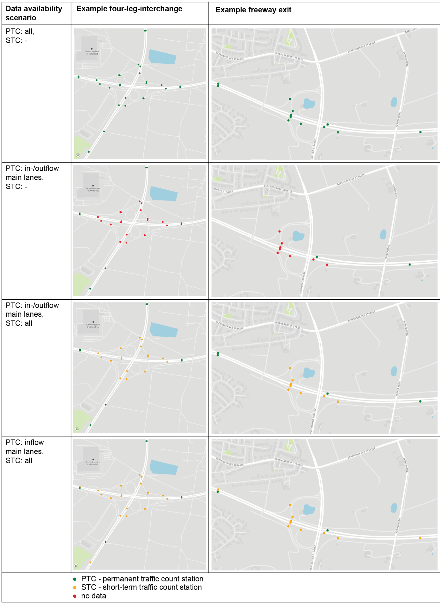
Data availability scenarios, applied to an interchange and a freeway exit.

Evaluation

For each ramp junction, the saturation rate is calculated for each DHV estimation scenario. For data availability scenarios with STC, every potential count day is simulated. As the resulting saturation rate differs depending on the day of the STC, an estimation scenario contains multiple saturation rates. Figure 4 shows exemplary results for one DHV estimation scenario, where each bar shows the result for one potential day of the STC. The saturation rate is represented by the height of the bar, whereas the color of the bar represents the LOS corresponding to the saturation rate. The target saturation rate of the reference scenario (50th highest saturated hour) is marked by the horizontal black line.

Figure 4.

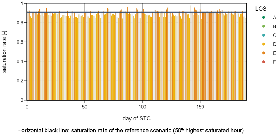
Example showing results of one ramp junction for a design hourly volume (DHV) estimation scenario with several short-term traffic counts (STCs) in one year.

The correlation between the saturation rate of the simulated STC and that of the reference scenario is shown in Figure 5. For each ramp junction of a node, the results of the simulated STC are plotted against the target saturation rate of the reference scenario (each bar of Figure 4 has a corresponding point in Figure 5). The results of one specific ramp junction are plotted on the same x-coordinate since the reference scenario does not depend on the day of the STC. The colored squares illustrate the corresponding LOS. If a point is located in one of the squares, the saturation rate of the simulated STC results in the same LOS as that of the reference scenario. Otherwise, the simulated LOS differs from the target LOS of the reference scenario.

Figure 5.

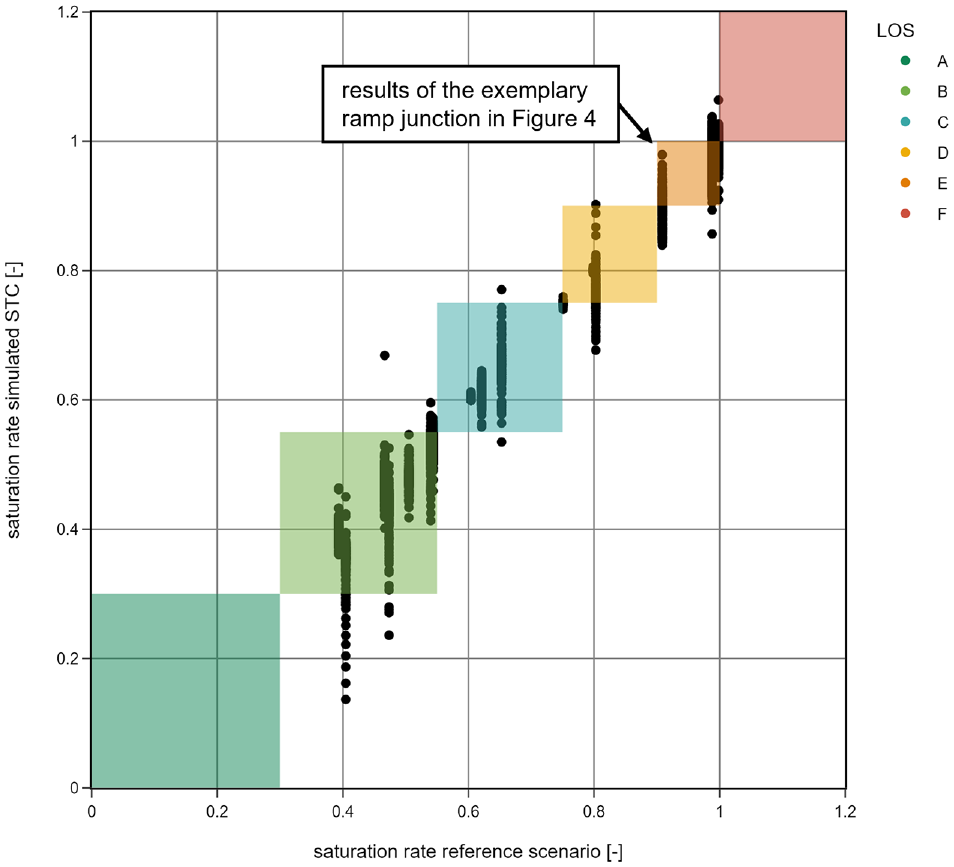
Example showing results of a node (with 16 ramp junctions) for design hourly volume (DHV) estimation scenario for several short-term traffic counts (STCs) in 2017.

Figure 5 shows the results for one node with 16 ramp junctions. To be able to evaluate the DHV estimation scenarios for all nodes, further aggregation of the results is required. For this reason, the metric of the “average LOS accuracy” is introduced. Based on the results of the simulated STC, this metric describes the relative share of the simulated STCs that achieve the target LOS of the reference scenario. In the visualization in Figure 5, this corresponds to the proportion of points located within one of the colored LOS-squares.

$$\mathrm{average}\mathrm{LOS}-\mathrm{accuracy}=\frac{n\left(LO{S}_{es}=LO{S}_{rs}\right)}{n}$$

(1)

where

$n=\mathrm{number}\mathrm{of}\mathrm{estimation}\mathrm{scenarios}$

$\mathrm{LO}{S}_{\mathrm{es}}=\mathrm{calculated}\mathrm{LOS}\mathrm{of}\mathrm{estimation}\mathrm{scenario}$

$\mathrm{LO}{S}_{\mathrm{rs}}=\mathrm{LOS}\mathrm{of}\mathrm{corresponding}\mathrm{reference}\mathrm{scenario}$

$\begin{array}{c}n(\mathrm{LO}{S}_{\mathrm{es}}=\mathrm{LO}{S}_{\mathrm{rs}})=\mathrm{number}\mathrm{of}\mathrm{estimation}\mathrm{scenarios},\mathrm{which}\mathrm{hit}\mathrm{the}\mathrm{LOS}\mathrm{of}\mathrm{their}\hfill \\ \mathrm{reference}\mathrm{scenario}\hfill \end{array}$

Results

Evaluation of the results for the years 2017, 2018, and 2019 shows similar values of LOS accuracy per year. The following discussion considers the results of all years (Table 2). Figure 6 shows the results for 2017 as an example. We aggregate the average LOS accuracy for each concept for DHV estimation (colored bars in Figure 6) with respect to the year and data availability scenario (x-axis). Figure 7 shows the results of Figure 6 split into results for interchanges and for exits.

Table 2.

Aggregated Evaluation for all Design Hourly Volume (DHV) Estimation Scenarios

Data availability scenario	Concept for DHV estimation	LOS accuracy			LOS under-estimation			LOS over-estimation			Without result
		2017	2018	2019	2017	2018	2019	2017	2018	2019	2017	2018	2019
PTC: all, STC: −	30th–70th hour (STC: frequent day hour)	96%	92%	94%	4%	8%	6%	0%	0%	0%	0%	0%	0%
PTC: all, STC: −	30th–70th hour (STC: mPH+aPH)	72%	78%	63%	1%	3%	1%	7%	5%	5%	20%	15%	31%
PTC: all, STC: −	50th hour (STC: day hour)	90%	92%	92%	2%	2%	2%	8%	6%	6%	0%	0%	0%
PTC: all, STC: −	50th hour (STC: mPH or aPH)	90%	92%	92%	2%	2%	2%	8%	6%	6%	0%	0%	0%
PTC: in-/outflow main lanes, STC: −	30th–70th hour (STC: frequent day hour)	42%	42%	41%	3%	4%	3%	55%	55%	55%	0%	0%	0%
PTC: in-/outflow main lanes, STC: −	30th–70th hour (STC: mPH+aPH)	39%	39%	38%	3%	4%	3%	59%	57%	59%	0%	0%	0%
PTC: in-/outflow main lanes, STC: −	50th hour (STC: day hour)	37%	38%	39%	2%	3%	3%	60%	58%	58%	0%	0%	0%
PTC: in-/outflow main lanes, STC: −	50th hour (STC: mPH or aPH)	38%	38%	40%	2%	3%	3%	60%	58%	58%	0%	0%	0%
PTC: in-/outflow main lanes, STC: all	30th–70th hour (STC: frequent day hour)	93%	90%	92%	5%	9%	6%	2%	1%	2%	0%	0%	0%
PTC: in-/outflow main lanes, STC: all	30th–70th hour (STC: mPH+aPH)	88%	87%	88%	6%	8%	6%	7%	6%	5%	0%	0%	0%
PTC: in-/outflow main lanes, STC: all	50th hour (STC: day hour)	90%	89%	90%	3%	6%	5%	7%	5%	6%	0%	0%	0%
PTC: in-/outflow main lanes, STC: all	50th hour (STC: mPH or aPH)	87%	87%	87%	6%	8%	9%	6%	5%	5%	0%	0%	0%
PTC: inflow main lanes, STC: all	30th–70th hour (STC: frequent day hour)	87%	83%	83%	10%	15%	14%	3%	2%	3%	0%	0%	0%
PTC: inflow main lanes, STC: all	30th–70th hour (STC: mPH+aPH)	81%	81%	82%	5%	6%	6%	14%	12%	12%	0%	0%	0%
PTC: inflow main lanes, STC: all	50th hour (STC: day hour)	85%	82%	85%	10%	15%	12%	5%	3%	3%	0%	0%	0%
PTC: inflow main lanes, STC: all	50th hour (STC: mPH or aPH)	82%	79%	81%	13%	18%	14%	5%	3%	3%	1%	0%	1%
PTC: −, STC: all (week)	STC PH week (one demand-situation)	61%	57%	56%	7%	9%	9%	32%	33%	35%	0%	0%	0%
PTC: −, STC: all (week)	STC PH week (worst case)	84%	81%	82%	9%	12%	12%	6%	6%	6%	0%	0%	0%

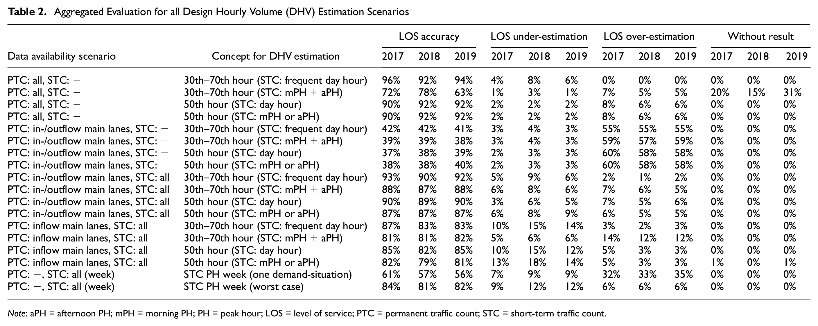
Note: aPH = afternoon PH; mPH = morning PH; PH = peak hour; LOS = level of service; PTC = permanent traffic count; STC = short-term traffic count.

Figure 6.

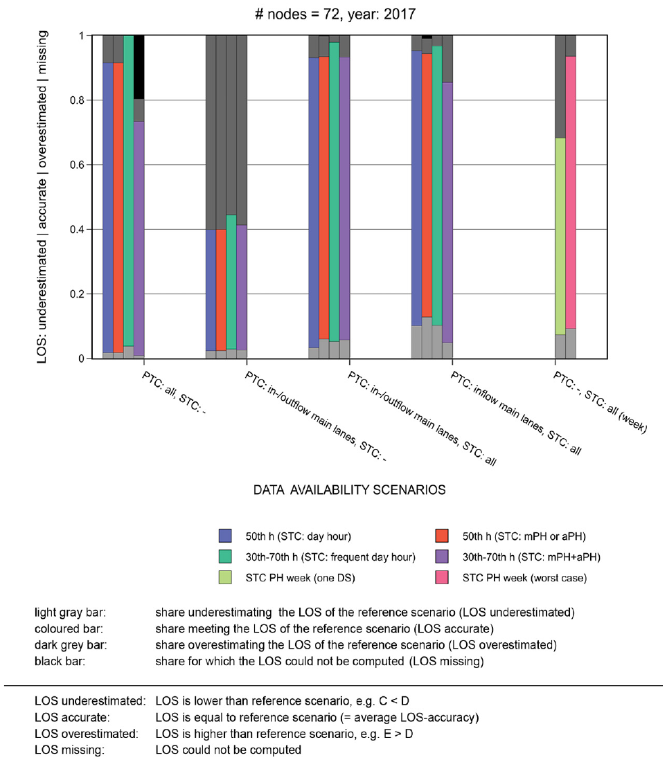
Aggregated evaluation for all estimation scenarios.

Figure 7.

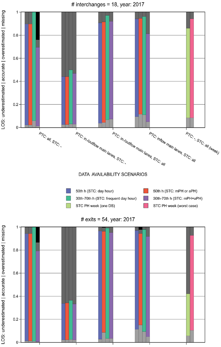
Aggregated evaluation for all design hourly volume (DHV) estimation scenarios by interchanges and exits.

PTC: All, STC: -

This data availability scenario shows the deviation of a concept for DHV estimation compared with the reference with perfect data availability, that is, PTC for all count stations. All concepts for DHV estimation perform quite similarly, with an average LOS accuracy of between 90% and 96%. An exception is the estimation concept “30th–70th hour (STC: mPH + aPH)”. The latter cannot compute a LOS for about 20% of the scenarios because of an inconsistent PTC demand-situation. That happens more often on interchanges than on freeway exits. An interchange has far more traffic streams and count stations, which lead to more boundary conditions for matrix estimation.

The results for the estimation concepts using the 50th hour as basic concept for DHV estimation are exactly the same, as the data availability scenario does not rely on STC. This is also a reason for the estimation concept “30th–70th hour (STC: frequent day hour)” having the highest average LOS accuracy. Calculating an average volume of multiple highly loaded hours is more robust compared with 50th highest saturation than just using the 50th hour as DHV. The number of scenarios that overestimated the LOS, especially, are reduced using the estimation concept “30th–70th hour (STC: frequent day hour)”.

PTC: In-/Outflow Main Lanes, STC: -

The reduction of available PTC in this data availability scenario leads to drastically decreasing average LOS accuracies for all concepts for DHV estimation. Most scenarios (about 60%) overestimate the LOS compared with the references, even more for nodes of freeway exit type. Without additional STC, there is no information about traffic stream distribution on ramps. Interchanges deal better with this availability scenario because there are PTCs on each inflow or outflow. For freeway exits, the traffic stream on ramps is overestimated.

PTC: In-/Outflow Main Lanes, STC: All

In this data availability scenario, STCs provide the missing information on the distribution of flows on the ramps. This leads to an improvement of the average LOS accuracy, up to 93%, which is near the result of the first data availability scenario “PTC: all, STC: −”. This approach works for interchanges and freeway exits, with exits having minor advantages because of their less complex topology. The estimation concept “50th hour (STC: day hour),” which derives the STC demand-situation based on the DHV of the PTC, has the fewest cases underestimating LOS compared with the reference. In contrast, the estimation concept “30th–70th hour (STC: frequent day hour)” shows the lowest share of overestimates. In this data availability scenario, there is little difference between the concepts for DHV estimation considering PTC demand-situations for each PTC station and the estimation concept “30th–70th hour (STC: mPH+aPH)” that creates artificial demand-situations for the morning and afternoon peak hours. Comparing this data situation with the previous availability scenario “PTC: in-/outflow main lanes, STC: −”, it is reasonable to conclude that additional information about traffic flows provided by STCs is crucial for a precise estimation of the LOS reference.

PTC: Inflow Main Lanes, STC: All

With the reduction of PTC stations, a decrease of the average LOS accuracy of about 5% to 9% can be observed for all concepts for DHV estimation. The three concepts that define multiple PTC demand-situations to maintain consistency tend to underestimate the LOS. In contrast, the estimation concept “30th–70th hour (STC: mPH + aPH)” tends to overestimate the LOS reference, especially for interchanges.

PTC: −, STC: All (Week)

The evaluation of the data availability scenario without PTC but with STC over a whole week shows that considering a demand-situation, including peak hours for all ramp junctions, overestimates the LOS in many cases, especially for freeway exits. The concept “STC PH week (worst case)”, which evaluates STC demand-situations for each ramp junction and considers a worst case per ramp junction, has an average LOS accuracy of almost 80%. This is similar to the result for the data availability scenario “PTC: inflow main lanes, STC: all”. This good LOS accuracy occurs because the idea of a weekly peak hour is quite equivalent to the 50th hour, considering that a year has 52 weeks.

Conclusions and Further Research

For the design of a traffic facility, the German HCM provides a concept for DHV estimation that determines the design hourly volume from the nth hour (usually n = 50) of a year. To determine this value exactly, the volumes of all traffic flows of a traffic facility must be recorded for all 8,760 hours of a year. The PTC stations required for this are usually only available on the main lanes in the freeway network, but not for ramps. For this case, the German HCM recommends determining the unrecorded ramp traffic volumes by means of STCs with a subsequent projection using the available permanent traffic counts.

The aim of the study is to develop concepts for DHV estimation at freeway nodes and to compare them with a reference concept based on the nth highest saturated hour of a year. When comparing the concepts, the available databases (PTC stations, STCs) are varied to examine how this affects the accuracy of an estimation.

Using a reference database, combinations of six concepts for DHV estimation and five data availability scenarios are tested. The study provides the following results on the databases:

• The data availability scenario has a much stronger influence on the quality of the results than the choice of the concept for DHV estimation.

• It is sufficient to have one PTC on each inflowing main lane of a freeway node.

• STCs on all ramps of the node are crucial for an accurate estimation of the DHV because this is the only way to collect information for all origin–destination flows at the node.

• The results indicate that the method proposed in the German HCM for determining the DHV at nodes using STCs and extrapolating at PTCs precisely meets the required nth highest saturated hour.

The results for the concepts for DHV estimation can be summarized as follows:

• The estimation concepts provide rather similar results for identical data availability scenarios.

• Estimation concepts defining STC demand-situations with regard to the PTC demand-situation—“50th hour (STC: day hour)” and “30th–70th hour (STC: frequent day hour)”—lead to slightly better results.

• Estimation concepts that use peak hours for the STC demand-situation—“50th hour (STC: mPH or aPH)” and “30th–70th hour (STC: mPH + aPH)”—have the disadvantage that the choice of the corresponding peak hour is dominated by the traffic volumes on the main lanes, since these lanes contribute most to the total traffic volume of the node. The traffic volumes of the ramps are underrepresented concerning their influence on the selection of the demand-situation, although they usually have a larger influence on the traffic flow quality at a ramp junction.

• Estimation concepts which only consider STCs of a week, that is, “STC PH week (worst case)”, can provide a good estimate for the nth highest saturated hour, if the counts are carried out in representative weeks (e.g., outside of holidays).

The results of this study are based on a reference database. This reference database is the result of a data processing approach in which missing data/traffic volumes were complemented by realistic values based on available PTC data in the vicinity. The concepts presented were tested on different traffic facilities (merging, diverging, and weaving segments of freeway exits and interchanges). The concepts and the influence of the availability scenarios (STCs, PTCs, or both) were evaluated in aggregate for these facilities. In future research, the influence of the concepts and data availability scenarios on the individual facilities should be investigated in more detail since the effects might differ for clusters of similar facilities. The same applies to the temporal aggregation: Figure 4 shows that the estimation accuracy differs depending on the day for which the STC is simulated. A careful identification of suitable days could further improve the method. In addition, the question arises of how other data sources, such as floating car data, would perform if these were used instead of short-term traffic counts.

The procedures used to calculate LOS in this study and the use of the saturation rate are taken from the German HCM. The traffic facilities evaluated are also located in Germany. In the future, it would be interesting to evaluate the method in other countries in combination with the guidelines applicable there (e.g., the HCM, which determines the LOS of a ramp junction based on traffic density).