
Abstract
The standard framework for evaluating the impact of online shopping on travel and shopping behavior considers the possibility of complementarity, substitution, neutrality, or modification effects. Complementarity (online shopping complementing physical purchases, or vice versa) and substitution (online shopping replacing trips to physical stores and eventually the stores altogether) have generally received more attention in research, particularly the latter, since substitution may substantially impact travel and street life within cities. This paper analyzes data from a two-wave seven-day shopping and travel survey implemented in Lisbon before the COVID-19 pandemic (January–February 2020) and in its aftermath (April–May 2022) using a structural equation model and multigroup analysis. The results show that, in 2022, variables such as education or income, often used to characterize online shoppers, have lost significance as predictors, suggesting a broader engagement with online shopping. Moreover, the complementarity effect found in 2020 has given place to substitution, which also supports that the physical–online shopping balance might have tipped toward a more generalized adoption of online shopping in the aftermath of the pandemic.
Keywords
The COVID-19 pandemic caused a huge disruption to everyday life. A global increase in the adoption of online activities was necessary to reduce the risk of infection ( 1 , 2 ), and social distancing measures forced people to become familiar with digital technology out of necessity ( 3 ). E-commerce, which accounted for 13.8% of retail sales worldwide in 2019, reached a share of 19.7% in 2022 ( 4 ). This huge increase in just three years may be a sign of things to come, although growth is expected to slow down, with forecasts indicating that online shopping will account for a quarter of global sales in 2026 ( 4 ).
During the peak of the pandemic, shopping online became more than a convenience; it became a way of avoiding dangerous supermarket queues ( 5 ). Health-related fears prompted consumers to shop more online ( 6 ), and because telecommuting was also encouraged, the implications for travel were severe, with the number of trips generally falling, along with the share of public transport ridership ( 2 , 7 ). Because most countries had generally lifted most restrictions at the time of writing (in the face of the global decline in reported severe cases of COVID-19 and deaths form the virus), we may now start assessing what proportion of these “pandemic behaviors” were out of sheer necessity and what will become prevalent as part of the new “post-COVID-19 normal.” Although e-shopping is still a fraction of the shopping that takes place on the high street, can we not expect a “democratization” of e-shopping ( 8 ), considering the strengthened relationship between consumers and the online channel?
Two questions arise from this scenario. The first pertains to the implications for individuals’ travel patterns. During the pandemic, online shopping increased, and many public transport users shifted to active modes and individual car use ( 9 – 11 ). The relationship between car use and online shopping had been noted in research before the pandemic ( 12 , 13 ). Online purchases may be complemented by physical purchases ( 14 , 15 ), eventually made by car ( 12 ). If the pandemic strengthened this relationship, what will be the consequences for promoting sustainable travel patterns and a “car-free lifestyle”? A second question relates to the consideration that not everyone can shop online: age (younger) and education (and, to a lesser extent, gender and income) played a significant role in the adoption of e-shopping ( 16 – 18 ). Will older, poorer, and less well-educated consumers be left out of this “e-shopping revolution”?
To contribute to this discussion, we compare a shopping survey (here termed the Lisbon Shopping Survey [LSS]) implemented in Lisbon in two waves, that is, immediately before the pandemic (January–February 2020) and approximately two years later (March–April 2022) when most restrictions had been lifted. The survey characterizes the respondents considering socioeconomic characteristics and other variables that influence shopping and travel. The LSS also incorporates a seven-day shopping diary and an evaluation of individual preferences with regard to shopping (Likert scale questions). The longitudinal before-and-after COVID-19 data may provide relevant insights into long-lasting changes in shopping and travel patterns. In this paper, we use “e-shopping” and “online shopping” interchangeably, referring only to the purchase, not the search processes. We believe that time-use surveys are better suited to the study of the latter.
This paper is organized as follows. A brief literature review is presented in the next section, followed by a description of the data and methodology. Then, a structural equation model (SEM) using the 2020 specification ( 12 ) is implemented using 2022 data, and a multigroup analysis is performed to compare it with the 2020 results ( 12 ). The results are discussed, and the paper finishes with the conclusions and some guidelines for further research.
Literature Review
The first COVID-19 lockdown has been called “the largest work-from-home experiment” ( 19 ). In the first year of the pandemic, out of fear of contracting the disease ( 2 ) but also because of the possibility of working from home ( 10 ), it seemed we left traffic jams behind and headed back to living in small neighborhoods; some people even moved to the countryside ( 20 ). A fueled sense of community was apparent in the implementation of online neighborhood social networks ( 21 , 22 ), and because people engaged in physical activity in the neighborhood and nearby parks ( 23 ), and shopped at local independent small shops ( 24 ).
However, although support for local small shops increased, visits to grocery shops decreased by as much as 34% between February 15 and April 17 2020 in Japan ( 25 ). In the Netherlands, the proportion of respondents who shopped for groceries at physical stores at least four times a week dropped from 15% in September 2019 to 8% in late March/early April 2020 ( 10 ). In Istanbul, the frequency of grocery shopping (in-store purchases) dropped by 17.1% from January 2020 to April 2020 ( 26 ). The increase in e-shopping may have offset the potential growth in “going local,” which was also in part a result of working from home ( 24 ).
The impact of e-shopping on travel has been analyzed since the advent of the internet made it as attractive as home shopping television channels or catalog shopping had been before ( 27 ). E-shopping presents the consumer with an unlimited selection, lower prices/search costs, and the convenience of shopping from home, among other desirable features ( 27 ). On the other hand, online shopping cannot offer, for example, sensory information or immediate possession ( 27 ). The former is one of the significant advantages of physical stores over online shopping and, ultimately, may be the determining factor in keeping retail on the streets ( 28 ). The latter will become less advantageous as deliveries become faster. For example, in California, the percentage of frequent users of priority shipping for e-shopping purchases increased from 14.23% to 24.21% when comparing 2020 with 2019 ( 29 ). The positive impact of same-day delivery in relation to the substitution of physical shopping for online shopping has also been discussed in previous research, even before the pandemic ( 30 ).
The potential impacts of online shopping on in-store shopping, namely, substitution, complementarity, modification, or neutrality, as framed by Mokhtarian ( 27 ), have frequently been analyzed using SEM ( 31 – 35 ). Weltevreden ( 36 ) proposes that complementarity results from e-shopping leading to shopping in store (for example, because of promotions online that require a visit to the store or, generally, because physical purchases can complement e-purchases). On the other hand, substitution always implies that an online purchase replaces a trip to the store ( 36 ) (from the consumer’s point of view, because the delivery also results in a trip). These two effects have generally been more evident and, therefore, received more attention in research than neutrality (no effect of online shopping on physical purchases and trips) or modification (changes in trip chaining and scheduling). This focus has also happened because substitution is bound to have an impact on travel and street life within cities.
Individuals’ socioeconomic characteristics matter in the decision to shop online. Apart from age, education, and income, research has also linked e-shopping with other individual factors such as holding a driver’s license, having access to a car, internet use and experience, and being responsible for the household shopping (shopping responsibility) ( 16 , 37 , 38 ). Shopping-related attitudes also influence the decision to shop online or in store, and “shopping enjoyment” has been related positively to the frequency of in-store shopping ( 39 ). Online shopping reveals a more utilitarian motivation ( 39 ) and is eventually motivated by a tighter time budget and a higher cost sensitivity than by the “pleasure of shopping” ( 40 ).
This heterogeneity among shoppers can eventually lead to different effects within a sample of respondents ( 18 , 35 ). Therefore, “time-pressured” respondents will be more likely to replace shopping trips with online purchases ( 35 ). At the same time, traditional shoppers will eventually continue to shop in store (neutrality), and dual-channel shoppers will complement physical shopping with online shopping ( 35 ). Similar behavior has been noted before (the “store shopaholics” versus “time-starved worriers” [ 18 ]), and also in Lisbon ( 12 ), and this is partly the reason we undertook the research presented in this paper. We wanted to evaluate what impact COVID-19 has had on shopping–travel relationships.
Therefore, in Lisbon, a SEM analysis implemented using data from the LSS 2020 ( 12 ) found that older, less well-educated, and more centrally located respondents preferred to buy in store and did so. On the other hand, younger, more educated, and car-dependent respondents preferred to buy online. The latter group revealed complementarity between online shopping on weekdays and in-store shopping at weekends, implying that a tighter time budget could be influencing their shopping behavior ( 12 ). Therefore, the research presented in this paper was designed to assess the impact of the COVID-19 pandemic on these relationships and link them with the promotion of the “car-free lifestyle” and equity in access to goods.
Data and Methodology
Research Hypothesis
The research hypothesis is built considering the literature and previous findings in relation to Lisbon ( 12 ). Although we still expect that a positive attitude toward online shopping might lead to more of it, with the same being true for a positive attitude toward in-store shopping and subsequent in-store purchasing, we now wonder if the relationship between those variables remains the same. Will the “loyal” in-store shoppers (who preferred to shop in store and did so, with their preference having a negative effect on online shopping) continue to be as loyal, or did COVID-19 pave the way for the adoption of widespread e-shopping? In addition, how did the relationship with other (exogenous) variables change? Is the online shopper still young, well educated, and affluent?
Therefore, the attitudes toward shopping enter the SEM as latent constructs (online shopping preference and in-store shopping preference) of Likert scale questions included in the survey to address these aspects. Because the 2020 model ( 12 ) revealed that shopping and travel behavior differed between weekdays and weekends, online and in-store purchases during these two periods will also enter the model as endogenous variables. Finally, sociodemographic variables, internet experience, mobility, and shopping opportunities will enter the model as exogenous variables too. The conceptual model, which considers the possible relationships between weekday and weekend shopping and between shopping behavior and shopping preferences, is presented in Figure 1 and will be tested using an SEM.
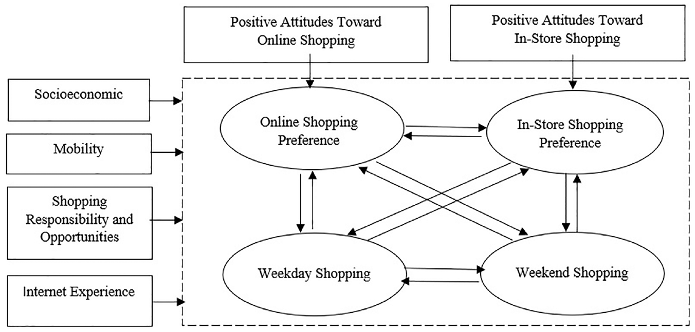
Conceptual model.
Figure 1 represents our starting point, from which different model specifications were developed. We started by testing one hypothesis and analyzing its statistical significance and the intuitiveness of the result (the first hypothesis being that preference for one shopping channel affects purchases using that channel on weekdays and weekends and also affects the preference for the other shopping channel). Because we were not satisfied with the model fit of this first attempt, and also because we were trying to get to a structure comparable with that of the 2020 data set (12), other hypotheses had to be tested before reaching the final specification. The conceptual model represents the many structures that might have been found in the data, and we do not want to give the impression that all these relationships were or should have been estimated simultaneously. They are all presented in Figure 1 to give the general idea that they were all possible within different specifications and that most were pursued until arriving at the final model, whose fit satisfied us and was also comparable with the results obtained from the 2020 data set (12). The final model structure and overall results are presented in the Results section.
Case Study and Data
Data used in this paper come from a two-wave seven-day shopping and travel survey implemented in Lisbon. The first wave was implemented between January and February 2020, immediately before the COVID-19 pandemic, and the second wave was conducted between April and May 2022, when most pandemic restrictions had been lifted. Working from home, for example, ceased being recommended altogether in the middle of February 2022 ( 41 ). The 2022 survey was implemented approximately two months later to give the respondents time to adapt to the new normal, which was almost free of restrictions.
The survey was implemented in Lisbon (the municipality), which is the capital and most populous city in Portugal, with a population of 545,796 residents (2021 census) ( 42 ). The respondents were recruited from an opinion panel, thus controlling the sample for gender and age (quota sampling). A pre-recruitment email was sent to a panel of 2,043 respondents in 2020, of which 1,648 demonstrated their willingness to participate. Considering the sample design (quota sampling for gender and age) and the completeness of the answers, we received 400 valid responses. In 2022, 2,431 respondents were pre-recruited and 1,847 demonstrated their willingness to participate, and again considering the sample design and the completeness of the answers, we received 400 valid responses, of which 80 were from respondents who had also participated in the first wave (2020). The age of the respondents ranges from 18 to 70, and the sample is representative of the population, considering age and gender.
Although only 20% of the panel returned for the second wave, the two samples are as similar as possible, not only in relation to age and gender but also with regard to education, employment status, income, and other variables that may influence purchasing and shopping channel choices. The survey is divided into three parts: characterizing the respondent; weekly shopping patterns (e.g., in-store and online shopping frequency) and shopping trips; and attitudinal aspects of in-store and online shopping. Likert scale questions are used. In wishing to provide an overview of the consumers’ shopping patterns and considering the need to span a period when different products might have been purchased, the survey addressed purchases made during one week. Other surveys on shopping patterns and travel implemented in Lisbon consider only one day, which is insufficient for addressing intrapersonal variability, for example ( 43 ).
Additionally, to avoid potential forgetfulness and underreporting of trips ( 44 , 45 ), every purchase was registered considering one of 17 possible categories of goods based on the official Portuguese Classification of Economic Activities ( 46 ), similar to the North American Industry Classification System. Retail ranged from supermarket purchases to household articles (e.g., furniture and home decoration items) to electrical and electronic appliances, in a total of 14 categories. Purchases made at restaurants, cafes, and bars accounted for the three remaining categories. However, in the end, we only considered retail items bundled as a whole because there were not sufficient purchases to model each category separately. Moreover, we considered that restaurants, cafes, and bars should be left for later (and eventually compared with retail, for example) to make the current analysis more straightforward.
Table 1 presents the definitions and descriptive statistics of the variables.
Definitions and Descriptive Statistics of the Variables
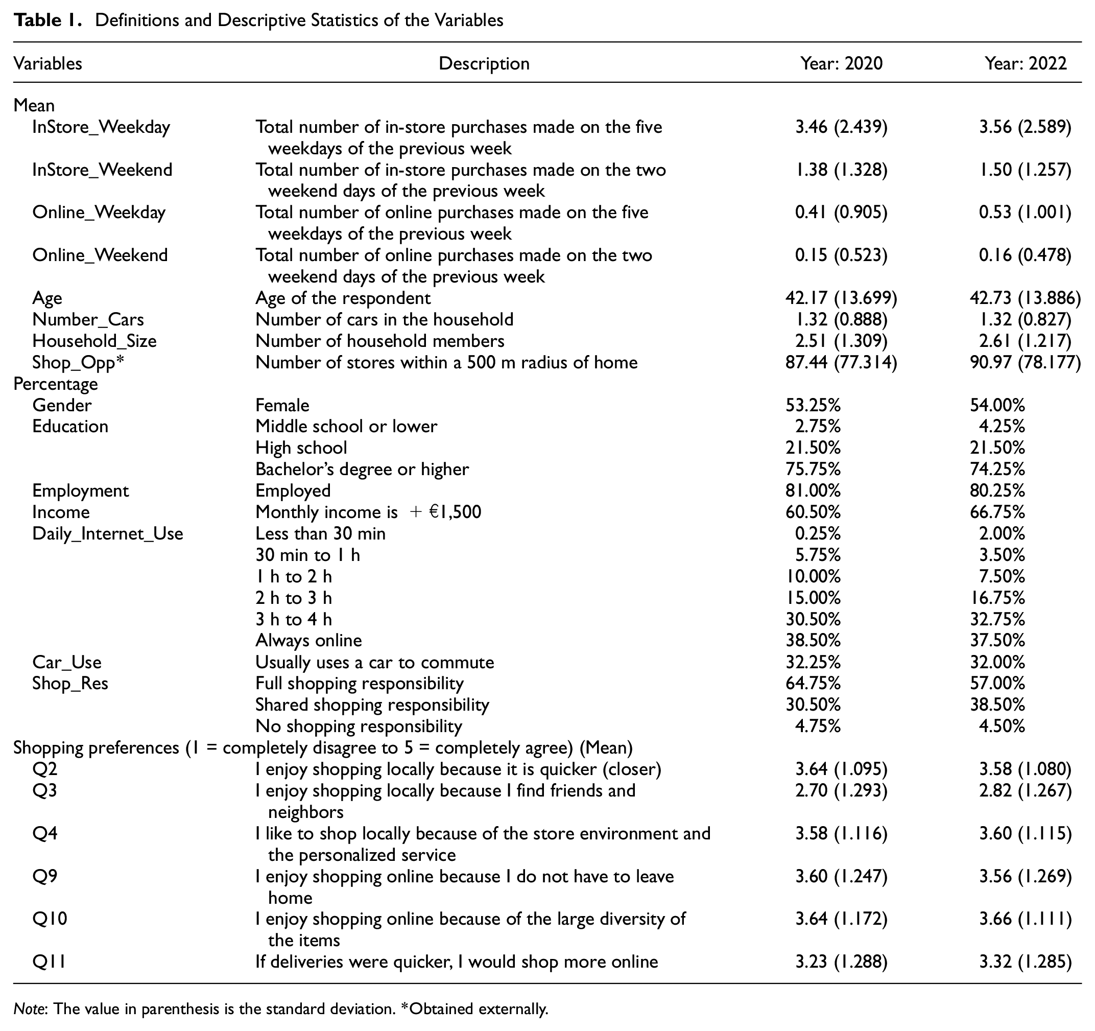
Note: The value in parenthesis is the standard deviation. *Obtained externally.
Although representative of the population considering age and gender, the sample presents more highly educated people in both waves, which can lead to a bias toward more e-shopping. When considering the two waves, people’s income is higher in the second, whereas the percentage of respondents having full responsibility for household purchases is lower. Even though to some extent we can expect the second to offset the first in the total number of purchases, the patterns and products might not be the same (e.g., less affluent respondents with full shopping responsibility buying groceries once a week and more affluent respondents with less shopping responsibility also buying once a week, but purchasing leisure items). This difference will be kept in mind during the discussion of the results.
Methodology
The empirical data are analyzed using SEM and employing Bayesian estimation ( 47 ) as implemented in the AMOS 26TM software ( 48 ). SEM is a well-known statistical modeling technique adapted for modeling complex and indirect relationships and simultaneously accommodating latent variables. We direct the reader to ( 49 , 50 ) for more detailed information on SEM. The Bayesian estimation method uses a prior distribution, which is combined with the observed data, using Bayes’ theorem formula to estimate an updated version of the model parameters, which is called a posterior distribution ( 48 ). This distribution reflects a combination of the initial belief (given by the prior distribution) and the empirical evidence ( 51 ), and is computed using Markov chain Monte Carlo simulation techniques ( 48 ).
The prior distribution used in the Bayesian estimation is based on a previous maximum likelihood (ML) estimation of the same model specification and data set. In this ML estimation, the following goodness-of-fit indicators were obtained: the comparative fit index (CFI) is 0.957, the normed fit index is 0.864, the non-normed fit index (NNFI) is 0.942, the root mean squared error of approximation is 0.031, and the standardized root mean square residual is 0.049. The simulation stops when the model achieves stability in the estimated parameters. In the AMOS module of SPSS, this is assessed by a convergence statistic, which, by default, should be smaller than 1.002 ( 47 , 48 ).
The model in this study contains both a measurement submodel and a structural submodel. It can be described by the following set of equations, where Equation 1 represents the structural submodel and Equation 2 the measurement submodel:


where
η is a vector (6×1) of latent endogenous variables,
B is a matrix (6×6) of coefficients of η variables,
Γ is a matrix (6×6) of coefficients of exogenous variables,
x is a vector (6×1) of observed exogenous variables,
ζ is a vector (6×1) of errors from structural relation,
y is a vector (6×1) of observed endogenous variables,
Λy is a matrix (6×6) of regression coefficients of y on η, and
ε is a vector (6×1) of measurement and errors on y.
The model outputs include the average value of the posterior (posterior mean) distribution, that is, the posterior standard deviation, similar to the conventional standard error ( 47 , 48 ) and confidence intervals. What is calculated is not exactly a confidence interval but a Bayesian credible interval, which has better properties than the conventional confidence interval if the posterior distribution is not normal ( 48 ). The same model specification was used for 2020 and 2022 and compared using multigroup analysis afterwards. Multigroup analysis is more robust than simple fit and parameter comparison, because it tests for the simultaneous invariance of several model parameters (measurement weights, structural weights, covariances, and residuals) between different populations ( 52 , 53 ).
Results
The model fit is indicated by the predictive posterior p-value (ppp). The ppp is a Bayesian counterpart of the classic p-value ( 54 ). A ppp close to 0.5 indicates that the model is plausible, because its discrepancies are closer to the center of the posterior predictive distribution of the discrepancy measure ( 55 ). Values close to 0 or 1 indicate a worse fit ( 56 ). Because the ppp is not uniformly distributed, it has no theoretical cutoff to maintain Type I error at 0.05 as p-values do ( 57 ). However, the 0.05 cutoff has been used to maintain consistency with traditional p-values ( 57 ). Because the ppp equals 0.06, the model is considered to have an acceptable fit. Additionally, the ML estimation fit indicators CFI and NNFI are used to help compare the models (>0.90 indicates a good fit) ( 58 , 59 ).
Therefore, in the 2020 model ( 12 ), ppp equaled 0.18, suggesting that the 2022 model fits the data less adequately (ppp of 0.06). Although the CFI and NNFI indicate a good fit in both models (>0.90), they are slightly worse considering the 2022 model. The CFI is 0.957 (0.976 for the 2020 model), whereas the NNFI is 0.942 (0.968 for the 2020 model). However, there is no suggestion that we should discard the 2022 model, although it has a worse fit than the 2020 model. Therefore, because we aim to compare changes in the relationships between variables in 2020 and 2022, we accept both models and proceed with the analysis.
Table 2 presents the measurement equations for the latent constructs of in-store shopping preference (InStore Preference) and online shopping preference (Online Preference) in 2022. InStore Preference is a latent construct of the attitudinal variables Q2, Q3, and Q4, which reveal a positive attitude toward in-store shopping. Online Preference is a latent construct of the attitudinal variables Q9, Q10, and Q11, which show a positive attitude toward online shopping. All the other attitudinal variables included in the survey were excluded from the latent variables because they reduced the fit of the preliminary exploratory factor analysis and the measurement submodel in 2020. Therefore, they were also excluded in 2022.
Measurement Equations for the Latent Constructs InStore Preference and Online Preference (2022)
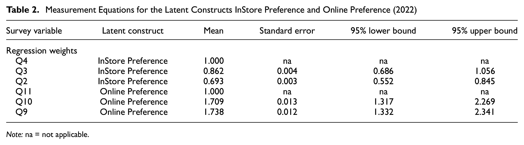
Note: na = not applicable.
Table 3 presents the standardized direct effects of one variable on another and the total effects (the sum of the direct and indirect effects) in 2022. InStore_Weekday and InStore_Weekend represent physical purchases made on weekdays and at weekends, respectively. Online_Weekday and Online_Weekend represent online purchases. Some of the variables shown in Table 1 are absent in the final model. They were excluded for model fit purposes in 2020 ( 18 , 31 ), and because the model in 2022 uses the same specification, they were not considered for this either.
Direct and Total Effects for the Adopted Model (Standardized) (2022)
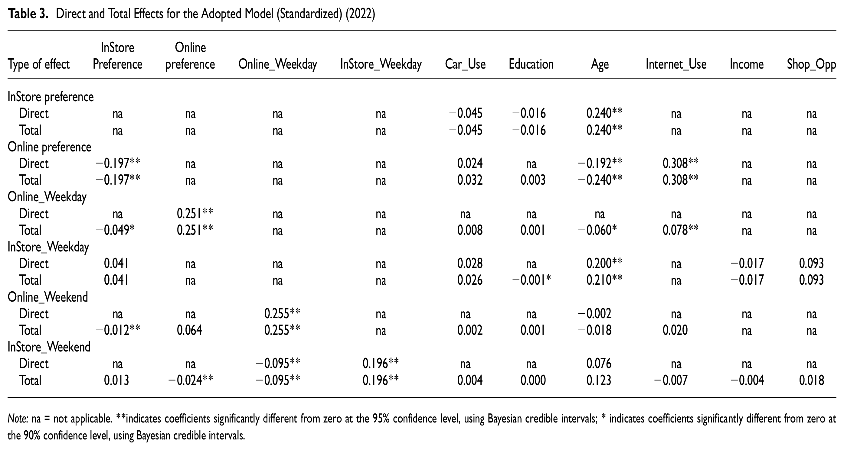
Note: na = not applicable. **indicates coefficients significantly different from zero at the 95% confidence level, using Bayesian credible intervals; * indicates coefficients significantly different from zero at the 90% confidence level, using Bayesian credible intervals.
Results from the multigroup analysis are presented in Table 4.
Multigroup Analysis*
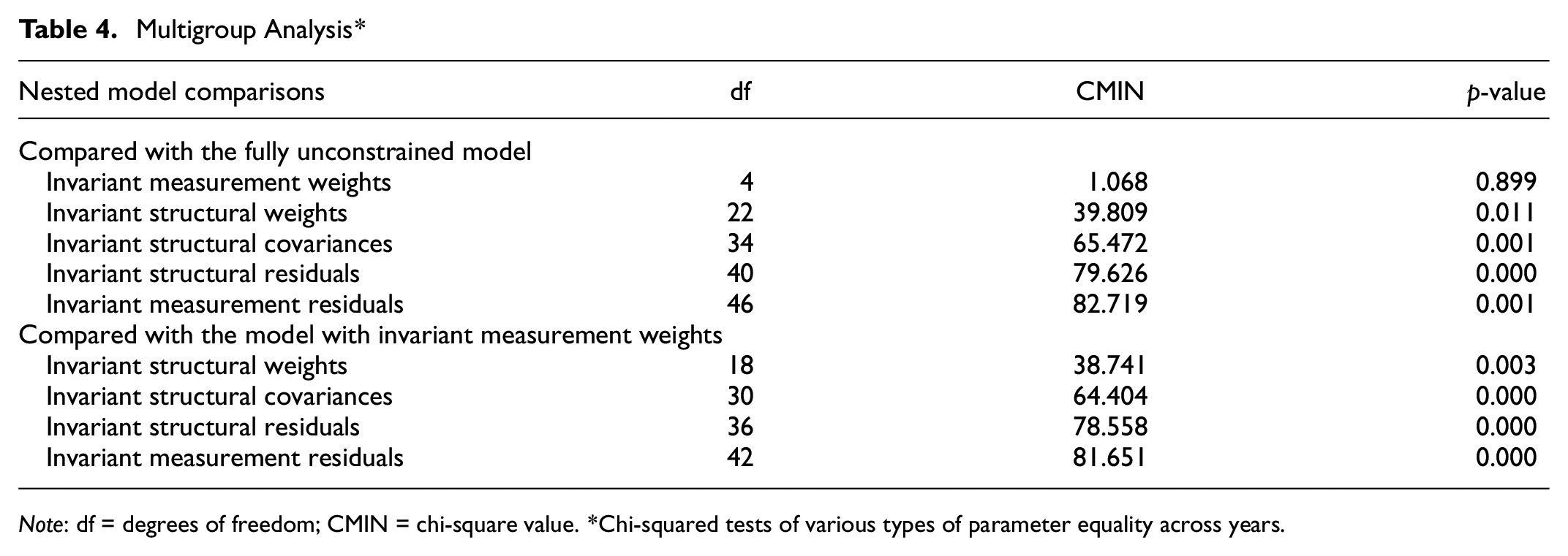
Note: df = degrees of freedom; CMIN = chi-square value. *Chi-squared tests of various types of parameter equality across years.
The unconstrained model, in which all parameters are freely estimated in each group, suggests the hypothesis indicating the measurement weights will be the same in 2020 and 2022 cannot be rejected, whereas for all the other parameters, this hypothesis is rejected. Additional restrictions are made, and the measurement weights are constrained to be equal across both groups. In this latter case, the hypothesis of invariance across groups is rejected for all parameters. Therefore, the model effects shown in Table 3 can be assumed to be different from the ones found in 2020, and this is discussed in the following section.
Discussion
Analysis of the 2020 model ( 12 ) showed that in-store preference was significantly related to age (positively) and education and car use (negatively), suggesting that shopping in store could eventually be linked with an older and less well-educated group that did not commute by car, and was more centrally located (closer to more abundant “shopping opportunities”). The latter was supported by the positive effect of shopping opportunities on in-store purchases on weekdays and at weekends (although not significant for the latter). On the other hand, online preference could be related to car use, internet use (positively), and age (negatively), suggesting that a younger population that commuted by car and was, therefore, eventually more peripherally located, was more likely to shop online. Considering that online shopping on weekdays showed a positive and significant effect on in-store purchases at weekends, eventually related to a tighter time budget during the week, a complementarity effect between online and in-store purchases was evident and found to be related to this younger, more peripherally located group ( 12 ).
In 2022, these relationships were lost to some extent. Age still has a positive impact on in-store preference and a negative impact on online preference (both are significant). However, the total effect of age on online purchases is smaller and less significant on weekdays and nonsignificant at weekends. The effect of age on in-store purchases at weekends has also ceased to be significant. This loss of significance may be happening because in the sample, there are more online shoppers in all groups aged 35+ and more online purchases per individual for all groups aged 45+.
On the other hand, the effect of education and car use lost significance considering in-store preference, with the same happening for the latter considering the actual purchases. The magnitude of the effect of internet use on both online preference and online purchases on weekdays is greater in 2022, showing that the higher the level of internet engagement, the more likely people are to browse for products and then buy them ( 31 , 33 , 60 ). The suggestion from the 2022 model is that of a broader engagement with online shopping by all kinds of respondents. Figure 2 presents the empirical relationships between endogenous variables in 2020 ( 12 ) and 2022, which also supports this idea of a potential “democratization” of e-shopping as the COVID-19 pandemic progressed ( 8 ).
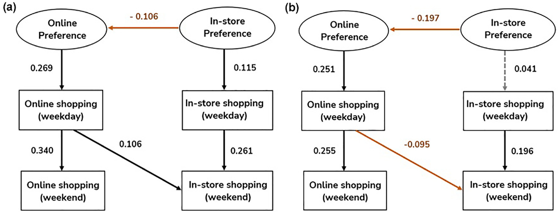
Empirical relationships between endogenous variables (standardized direct effects): (a) 2020; (b) 2022.
Figure 2 shows that although in-store preference still has a negative impact on online preference, it ceased to have a significant impact on in-store purchases on weekdays. Whereas in 2020, a group of “loyal in-store shoppers” preferred shopping in store and did so, in 2022, this loyalty has been shaken. A possible conclusion is that although people still prefer to shop in store, the group that only shops via this channel has become smaller. Therefore, the effect on physical purchases became nonsignificant. Additionally, as online shopping became (more) widespread, some people may still prefer shopping in store although they shop via both channels.
Perhaps the most impactful change is that the complementarity effect found in 2020 has also been lost. Younger people who commuted by car, shopped online during the week, and complemented those purchases efficiently with in-store shopping at weekends, can no longer be found by the model. Because the 2022 model shows a negative relationship between shopping online on weekdays and in store at weekends, they may have gone entirely online. However, we cannot say this group is the same because although the effect of car use on online purchases is still positive, it is nonsignificant. We can expect that the group of car commuters is now found among the much larger group of 2022 online shoppers.
Conclusions
This paper implemented an SEM to analyze the relationships between online and in-store shopping preferences and purchases in Lisbon, Portugal. For the purchases, we considered all products (retail) reported from a one-week shopping diary kept by 400 respondents during April and May 2022 (two months after most COVID-19-related restrictions had been lifted). For this analysis, the products were bundled together (all categories) and then divided according to the purchase period, that is, weekend or weekday. The material and methods (survey design and implementation, data curation, SEM) are the same as the ones used in a similar analysis implemented in 2020 ( 12 ). Finally, although the samples are not the same (only 20% of the panel returned), they are matched in relation to most socioeconomic variables and other factors that influence online shopping.
Considering the changes between 2020 and 2022, a broader engagement with online shopping is evident. Variables such as age and education, traditionally used to separate the online shopper from the in-store shopper ( 16 , 17 , 31 ), do not have the same impact as they used to. We found age to be significantly related to a preference for buying in store but not as significantly related to the actual physical purchase at weekends. Older respondents are also less resistant to shopping online: the negative effects of age on online shopping are less significant (weekdays) or nonsignificant (weekends).
As for the “loyal in-store shoppers” found in 2020 who were older, less well educated, and centrally located, they have “disappeared” from the sample, either altogether or because they are now part of a larger group of respondents who buy in store and online. The preference for buying in store also ceased to affect the purchase significantly. Although respondents still prefer to shop in store, this does not necessarily translate into a purchase, supporting the widespread adoption of online shopping.
Another finding is that the complementarity relationship between online purchases on weekdays and in-store purchases at weekends found in 2020 has been replaced by a substitution effect in 2022. We bear in mind that the samples are similar but not the same; therefore, we may be dealing with somewhat different groups of people. Additionally, we are considering all retail items bundled together, and some in-store purchases may be more prone to substitution (or complementarity) by online purchases than others. Nevertheless, the model shows a general substitution of in-store shopping for online purchases in 2022, when it showed complementarity in 2020.
Therefore, considering the discussion up to this point, and also the literature on changing shopping and travel behaviors during the COVID-19 pandemic, we have to admit the possibility that as internet use and e-shopping adoption increased during the pandemic and people became more familiar with the options offered by online shopping, some purchases that were made via both channels may have shifted to online, with substitution being now more evident than complementarity (although the amount of online shopping is still a fraction of physical purchases).
Finally, multigroup analysis was used to compare the models, finding that although the measurement weights are the same, the structural weights are not. The measurement weights not being different indicate only that the relative importance of the various statements capturing shopping preferences remains constant for in-store and online preferences (InStore Preference and Online Preference). Therefore, we can hypothesize that the changes between 2020 and 2022 can be attributed to COVID-19 and its social distancing measures, which resulted in previous barriers to the adoption of e-shopping being eliminated.
Linking these results with the original questions and further research, the possible democratization of e-shopping could not be directly related to individual car use in 2022, as it could before the pandemic. In our sample, what increased was online shopping, but this did not necessarily mean a reduction in car use. Although individual car commuters may be part of a larger group that has replaced weekend shopping trips with online shopping, this may or may not lead to fewer trips, depending on what they do instead; for instance, they may engage in more travel for other purposes. The increase in priority shipping and same-day delivery during the pandemic ( 29 , 30 ) suggests that consumers may be less willing to wait for their purchases to be delivered efficiently, leading to more unnecessary trips (although from the logistics supply side). If the intention is to promote a car-free lifestyle, research must address other components of daily activity and the supply side to conclude if adopting online shopping will reduce travel.
With regard to equity in access to goods, the more negligible impacts of age and education on online shopping adoption point to a more “inclusive” experience that may help people with fewer shopping opportunities access goods. Here, we must remember that our samples are generally biased toward (more) educated individuals. Further research will address those hardly ever captured by online surveys: those who are poorer, less well educated, and older (+70). Not only can they be excluded from the e-shopping revolution, they may also generate more trips, or longer ones, because of their more peripheral residential location. The geography of the e-purchase ( 17 , 61 , 62 ) in relation to socioeconomic factors and the potential exclusion of citizens from online shopping will have to be addressed in further research, and it will eventually be necessary to engage with data from the entire Lisbon Metropolitan Area, where the core–periphery effect is bound to be more noticeable.
Footnotes
Acknowledgements
The authors would like to acknowledge Fundação para a Ciência e a Tecnologia (FCT) for Rui Colaço’s PhD grant SFRH/BD/136003/2018. This work was supported by national funds through FCT, reference UIDB/04625/2020, and in the framework of the project PTDC/ECI-TRA/4841/2021 (REMOBIL Research Project). We are grateful to the anonymous reviewers who helped improve this paper.
Author Contributions
The authors confirm contribution to the paper as follows: study conception and design: R. Colaço, J. de Abreu e Silva; data collection: Rui Colaço; analysis and interpretation of results: R. Colaço, J. de Abreu e Silva; draft manuscript preparation: R. Colaço, J. de Abreu e Silva. All authors reviewed the results and approved the final version of the manuscript.
Declaration of Conflicting Interests
The author(s) declared no potential conflicts of interest with respect to the research, authorship, and/or publication of this article.
Funding
The author(s) disclosed receipt of the following financial support for the research, authorship, and/or publication of this article: This work was supported by national funds through Fundação para a Ciência e a Tecnologia (FCT), reference UIDB/04625/2020, and in the framework of the project PTDC/ECI-TRA/4841/2021 (REMOBIL Research Project).
Data Accessibility Statement
The data used in this research is available from the authors on reasonable request.