
Abstract
This paper develops a model for quantifying the relationship between flight volume and its operational performance at the macro level and investigating whether there are any changes before, during, and after the pandemic. Inspired by the market basket concept from economics, we first calculate macro-level effective flight time (EFT) for the U.S. domestic flight market by constructing a flight basket. Semi-log-linear models are developed to formulate the relationship between the total number of flights and macro-level EFT and its components. The estimation results indicate that the total number of flights has a positive and significant impact on EFT and its components, with 29.244 min longer for the weighted EFT for the analysis period compared with a zero-traffic scenario. Further investigations into the post-pandemic period verify the performance of the model and indicate that deteriorating operational performance in this period, especially with regard to gate delay and taxi-in time, is not only a result of the recovery of the flight market.
Beginning in early 2020, COVID-19 had a negative impact on people’s willingness to fly ( 1 ), leading to dramatic changes in air transportation ( 2 ). Both flight volume and passenger load decreased dramatically ( 3 ), but traffic has recovered as the pandemic has abated. These dramatic fluctuations in traffic have affected the operational performance of air transportation ( 3 – 5 ).
The pandemic provides a natural experiment for investigating the relationship between flight traffic and operational performance. Traffic volume is one well-known factor that affects operational performance ( 4 – 7 ). However, many factors influence flight delays, and only some of these are closely linked with the levels of traffic in the system. Comparisons between operational performance in low- and high-volume traffic situations can reveal how much delay is volume related. This would allow for predictions of increased delay that would result from traffic growth in the future, and how much reduction in delay would be possible with capacity enhancements, which, theoretically, can eliminate volume-related delays. Additionally, the recovery in flight traffic arising from the reduced concerns about COVID-19 (a phenomenon that we term, somewhat loosely, the “post-pandemic recovery”), enables us to assess whether operational performance has changed in recent months in a manner that cannot be explained simply by an increase in flight traffic.
Many previous studies have analyzed flight operational performance. Metrics based on flight time are the most direct means of characterizing operational performance. Effective flight time (EFT) is one such metric. EFT is defined as the duration between the scheduled departure time and actual arrival time, and can be broken down into four components: gate delay; taxi-out time; airborne time; and taxi-in time ( 8 ). Definitions for these EFT components are as follows: (a) gate delay (the difference between actual departure time and scheduled departure time); (b) taxi-out time (the time between actual departure time and wheels-off time); (c) airborne time (the time between wheels-off and wheels-on); and (d) taxi-in time (the time between wheels-on and actual arrival at the destination gate).
Another commonly used metric for evaluating flight operational performance is arrival delay, calculated as the difference between the actual and scheduled arrival time, which is equivalent to the difference between the EFT and the scheduled block time. The EFT is a more reliable metric than the arrival delay for two reasons. First, scheduled block time changes over time ( 8 , 9 ). For example, the scheduled block time may be set longer to improve on-time performance. Therefore, the arrival delay may differ even for two flights with the same EFT. This means we should not directly compare arrival delays for the same flights at different times. Therefore, on-time performance based on arrival delay is not always reliable for operational performance analysis ( 9 ). Second, EFT provides more detailed information for different flight phases, allowing a more complete operational performance analysis by covering all flight phases.
Depending on the objective of the research, various approaches have been developed to analyze the operational performance of the air transportation system. Hsiao and Hansen ( 6 ) analyzed flight delays considering the effects of arrival queuing, volume, terminal weather, en route weather, and seasonal and secular effects. Wang et al. ( 8 ) compared the on-time performance of U.S. and Chinese airlines to investigate how different strategies in relation to setting scheduled block time affected operational performance. Dai et al. ( 7 ) included a broader scope of factors to model the system delay and predict days for which there was likely to be considerable delay, for example, queuing delays, terminal conditions, convective weather, wind, traffic volume, and special events.
This literature suggests that a high volume of traffic is among the most important reasons for poor operational performance ( 4 – 7 ). The total number of flights is an accessible and helpful metric for evaluating traffic volume at the macro level. Sun et al. ( 4 ) estimated the impact of the number of flights on the air transportation network during the COVID-19 pandemic. Zhou et al. ( 5 ) illustrate the vulnerability of the air transportation network, taking traffic volume into consideration. Thus, it is expected that flight volume will be a good predictor of operational performance. In Figure 1, we plot the weekly total number of U.S. domestic flights since January 2015. The volume of air traffic was fairly stable before COVID-19 but plummeted in the wake of the pandemic.
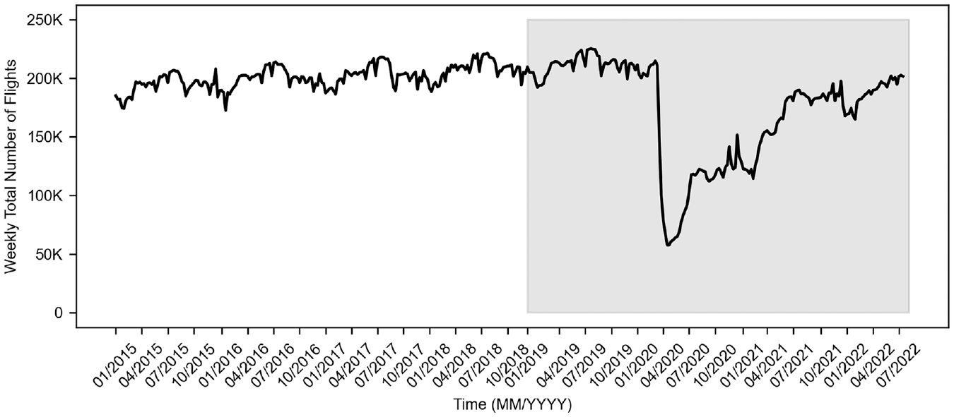
Weekly total number of domestic flights in the U.S.A. since January 1, 2015.
Although previous studies have yielded valuable insights into the relationship between air traffic volume and operational performance, none has developed a method for quantifying this relationship for all flight phases, or employed a data set that includes the large reduction in flight volume resulting from the pandemic. In this paper, we investigate how the operational performance across all flight phases is influenced by traffic, specifically during the pandemic period. Toward this end, we will focus on the relationship between flight volume and EFT, as well as the EFT components. Because flight traffic, that is, the total number of flights, is calculated for the whole flight system, we will analyze the relationship at the macro level. Specifically, we first borrow the market basket concept from economics and construct a flight basket to describe the EFT and its components at the macro level. Then, we develop regression models to formulate the relationship between the macro-level EFT and the total number of flights, while controlling for airport capacity and other omitted variable bias. The regression analysis is developed based on domestic flights in the U.S.A., for which the requisite data are readily available. Finally, we apply our models to the period of recovery following the pandemic. This serves two purposes. First, it tests model performance on out-of-sample data. Second, it reveals whether a high volume of delays during 2022 is simply the result of traffic recovery, as opposed to other factors, such as labor shortages, which are unique to the recovery period.
The remainder of this paper is organized as follows. We discuss the data source, construction of the flight basket, and the model specifications in the methodology section. Then, the estimation results are presented, and post-pandemic performance is discussed. Finally, we offer some conclusions and suggestions for future work.
Methodology
Data Source
We mainly use the Aviation System Performance Metrics (ASPM) flight-level data set in the Federal Aviation Administration’s (FAA) Operations and Performance Database ( 10 ). The data set provides departure date and time for each operating flight, location identifier for both departure and arrival airport, and components of EFT, including gate delay, and taxi-out, airborne, and taxi-in time, which can be used to derive variables needed for our analysis. The traffic volume and the EFT components can be aggregated at different spatial and temporal levels according to the flight, departure time, and departure/arrival airports. The location identifier for departure and arrival airports is used to construct airport origin–destination (OD) pairs for the operating flights of interest. In this study, the analysis period is from January 1, 2019 to July 25, 2022. All the variables needed are obtained or derived for this 186-week period.
Flight Basket
In economics, a market basket (
11
), that is, a selected group of goods and services, is usually used to measure price trends. The market basket for the Consumer Price Index (CPI) is the most popular application. The CPI is an index measuring the overall change in living costs, and is the primary measure of inflation. Prices of essential goods are constantly changing, and they are different for different goods. For instance, the price of clothes may increase by 5%, and the price of electricity may decrease by 3% in the same period. We cannot simply calculate the average changes for all kinds of goods because the amounts of different goods required are not the same. Assuming that the kinds and quantities of goods are held constant, researchers only need to calculate the weighted sum of the prices, with weights reflecting quantities that are purchased, to obtain living costs in different periods (
11
). The basket of all kinds of goods with proper quantities is the market basket, and the change in living cost is the CPI. CPI in the period

Inspired by the market basket, we can construct a similar metric as
To calculate the weighted EFT, we first need to identify a suitable basket that consists of a specific set of flights. Flights between specific airport OD pairs are treated as goods. Once a group of airport pairs is selected to form the flight basket according to our defined criterion, we calculate the weighted EFT (similar to
Similar to the
The Goods—Airport Pairs
To construct our flight basket, we must identify airport pairs that are consistently represented in our data throughout the analysis period. (We consider directional airport pairs—the A to B market is distinct from the B to A market.) Specifically, we include the airport OD pairs with at least
To make certain the criterion
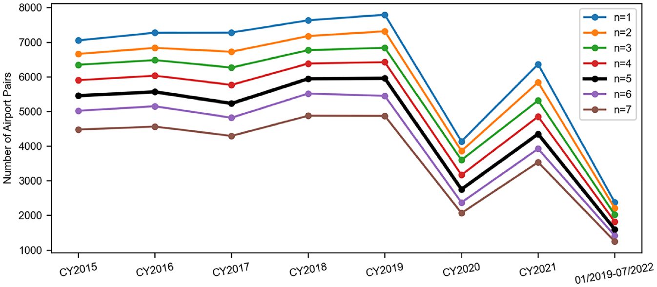
Trade-off between criterion n and number of airport pairs in flight basket.
The lines of different colors in Figure 2 represent different values of
The Total Cost—Basket-Level Weekly Weighted EFT
In this section, we will calculate the “price” and “quantity” of the selected airport pairs. These, in turn, are used to find the “total cost” of the constructed flight basket.
For the “price”, we compute the weekly (
(
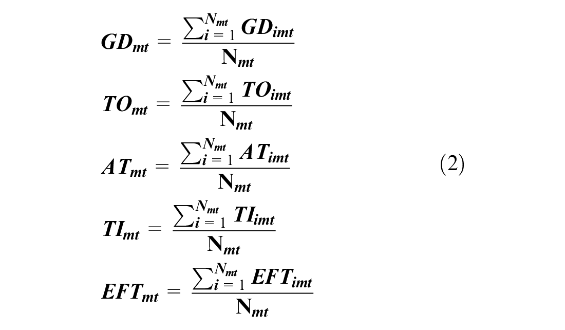
where
For the “quantity,” we use the total number of flights operating for a certain airport pair as the weight to reflect the consumption amounts for each airport pair. Intuitively, the more flights in one airport pair, the more contribution the airport pair makes to the market. We calculate the weights for each airport pair

where
Given the “amount” (i.e., the weights of airport pairs
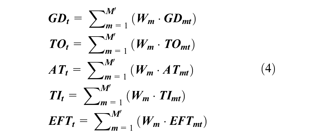
The calculation results for the flight basket-weighted EFT and its components for each week during the analysis period are shown in Figures 3 and 4. Figure 3 is the stacked bar chart showing the weekly weighted EFT and its components in different colors. Each bar represents the weighted EFT of one week in the analysis period, ranging from 120 to 140 min. We can see from the overall bar heights that there was a sharp drop around March 2020 when the COVID-19 pandemic started to affect the flight market. Each bar is also subdivided into its components. The airborne time accounts for most of the weighted EFT. To obtain a clearer view of the trends, we depict the time series for each component separately in Figure 4. Gate delay decreases during 2020 but increases in the post-recovery period compared with the pre-pandemic level. Taxi-in/out times share the same pattern as the total number of flights (Figure 1). The airborne time shows a periodic pattern but does not seem to be affected much by the COVID-19 pandemic.
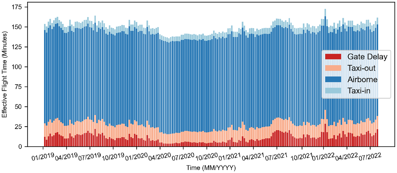
Weighted effective flight time for the flight basket.
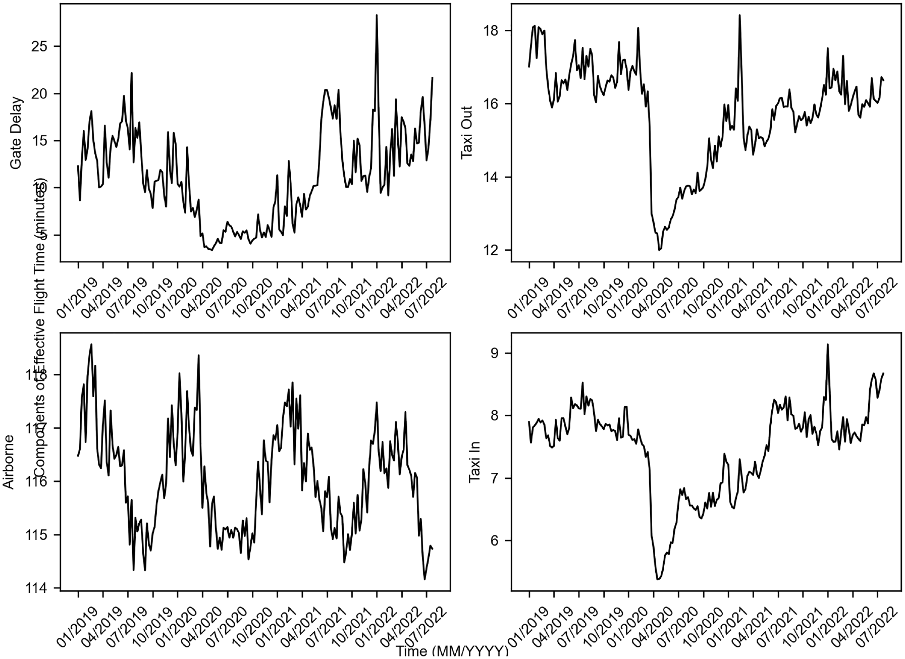
Components of weighted effective flight time for the flight basket.
Sensitivity Analysis
In the above sections, we have constructed the flight basket by selecting a group of airport OD pairs that have at least five flights operating every week of the whole analysis period, and have calculated the weighted EFT for the flight basket in each week. In this section, sensitivity analysis is conducted to illustrate that the construction period for the flight basket will not lead to a significant difference in the operational performance measures. By doing so, we can further verify the representativeness of the flight basket in relation to the whole aviation market.
Specifically, we calculate the abovementioned derived basket-level weighted EFT and its components for four flight baskets constructed for different periods with the criterion value
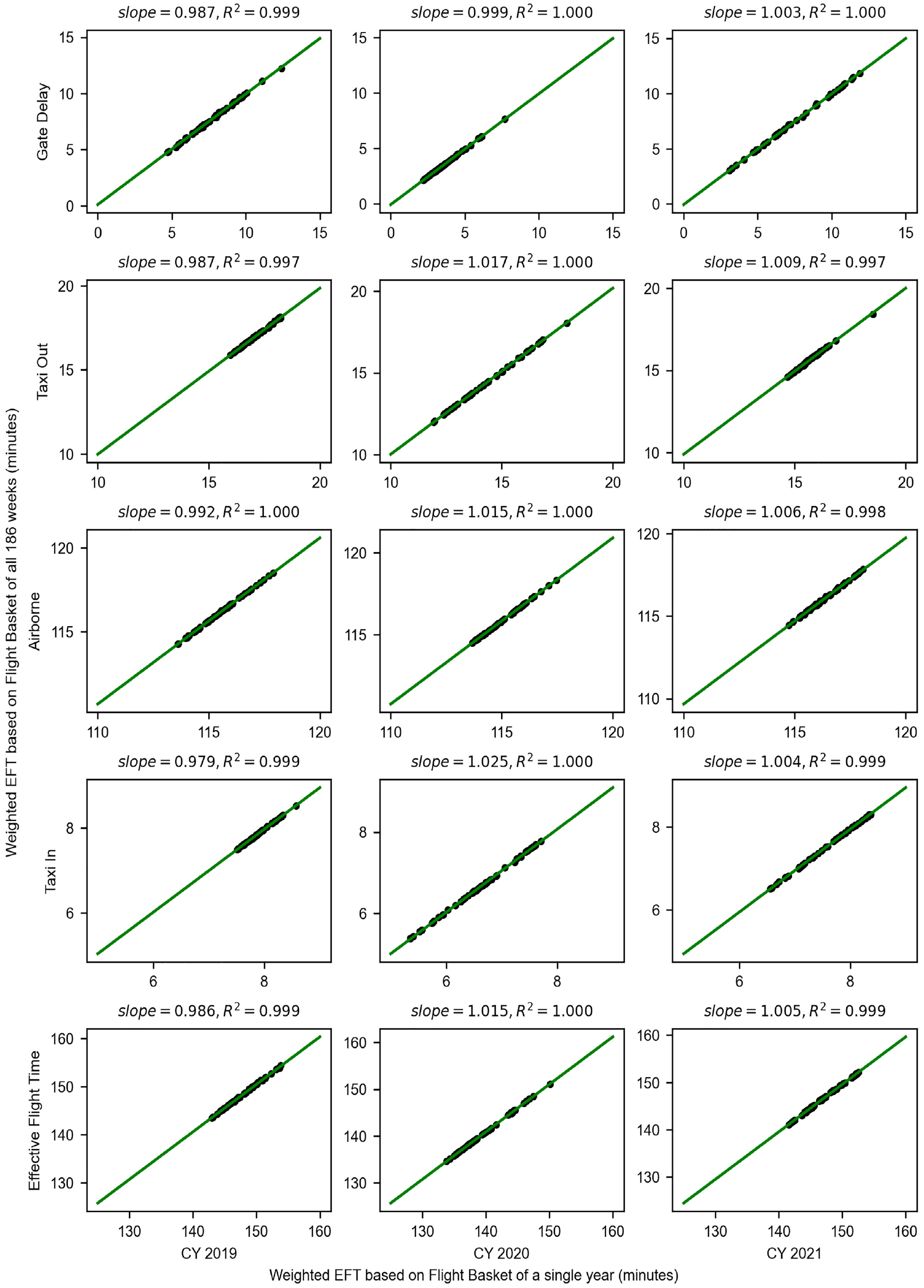
Weighted EFT comparisons for different flight baskets.
The
Regression Analysis
Model Specification
As discussed above, the construction of the flight basket helps make the operational performance metrics (i.e., weighted EFT and its components) comparable over time. In this study, we would like to understand further how and to what extent the number of flights may affect the weighted EFT and its components while controlling for omitted variable bias.
We perform initial investigations on data so as to discover patterns and spot the hypothesis we would like to test in statistical modeling. In Figure 6, we visually assess the relationship between the log-transformed weighted EFT and the total number of flights. Each point represents one observation of weekly weighted EFT and the total number of flight operations. There are 186 points in total over the analysis period, and the plot suggests a positive correlation between the two variables. This is expected, because increasing flight traffic exposes more bottlenecks in the National Airspace System (NAS), resulting in congestion. Moreover, the relationship when EFT is log-transformed appears to be roughly linear, suggesting an exponential relationship between EFT and flight traffic.
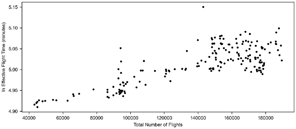
Relationship between log-transformed effective flight time and the total number of flights.
Thus, we estimate a semi-log-linear regression model to relate weighted EFT and its components to the number of flights and other factors. The model specification is formulated as in Equation 5, where

As well as the total number of flight operations
(
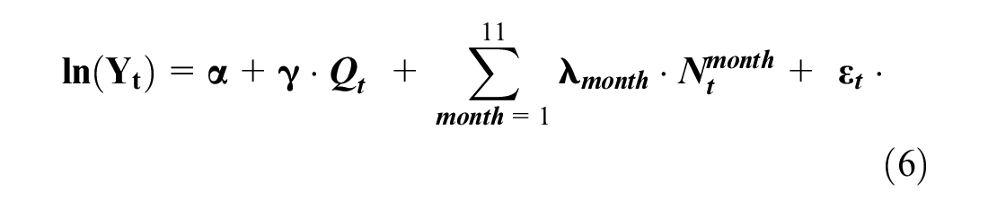
where
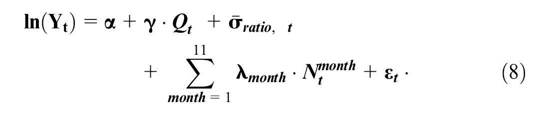
Airport Conditions
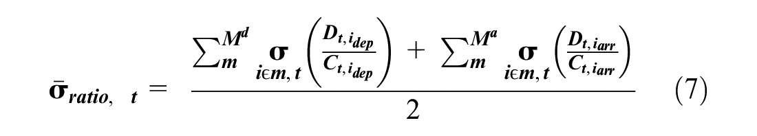
Apart from a high volume of traffic, adverse conditions at the terminal, such as congestion and bad weather, are also leading causes of poor operational performance. In this study, we employ the standard deviation of the airport demand-to-capacity ratio for departure and arrival to evaluate airport conditions for each airport pair. The demand-to-capacity ratio is a popular metric in transportation system analysis for describing the level of service. However, in our case, we found that the average value of the demand-to-capacity ratio is highly correlated with the total number of flights, with a correlation score of 0.88 for departure, and 0.90 for arrival, which leads to multicollinearity in our regression analysis. Intuitively, the greater the total number of flights, the higher the departure/arrival demand for each airport and, thus, the higher the demand-to-capacity ratio given that the capacity is relatively stable. Therefore, we employ the standard deviation of the demand-to-capacity ratio, which is less highly correlated to the total number of flights than the average, although it still captures imbalances between demand and capacity. If the standard deviation is high, then there are periods when the demand-to-capacity ratio is quite high, either because of reduced capacity or surges in demand; these are the conditions expected to cause a great deal of delay. Thus, the standard deviation of the demand-to-capacity ratio can be used to represent airport conditions and capture their impact on the weighted EFT.
We calculate the demand-to-capacity ratio for each flight for both departure and arrival airports based on quarter-hourly scheduled demand and capacity of the airport. In detail, we obtain the metric for airport conditions—the standard deviation of the departure/arrival demand-to-capacity ratio—in a manner similar to the method for obtaining the weighted EFT. First, because of missing data on demand and capacity for some airports, we obtained the new flight basket with

Results and Discussion
Estimation Results
In this section, we present the estimation results for the semi-log-linear model described in the previous section. We not only want to investigate the relationship between flight volume and operational performance, but also assess the ability of a model trained on data from the pre-pandemic and pandemic periods to predict performance in the post-pandemic period. Accordingly, we divide the analysis period, 186 weeks, into a 126-week training period (70%), from January 1, 2019 to May 31, 2021, and a 60-week test set (30%), from June 1, 2021 to July 25, 2022. Flight volume in the test period has substantially recovered from COVID-19. We make the split according to the time series for two reasons. First, it tests model performance on out-of-sample data. Second, we can determine whether a high level of delays in the post-pandemic period is simply the result of traffic volume recovery.
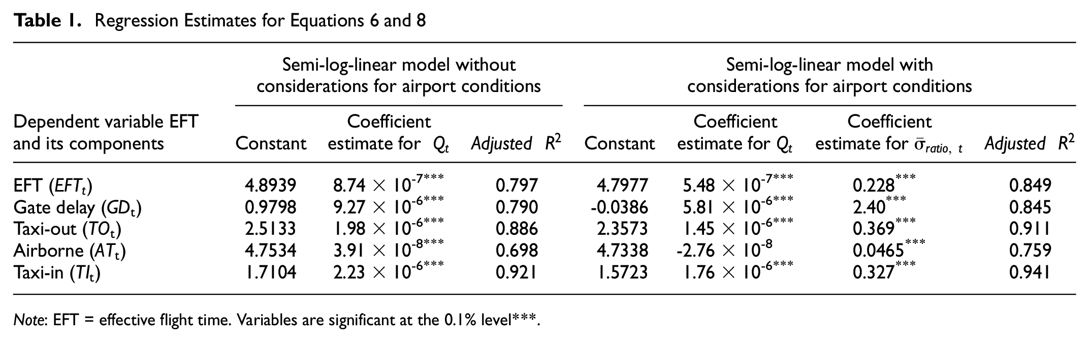
We estimate the variable coefficients of the semi-log-linear regression model specified in Equations 6 and 8 based on the training set for which the analysis period is from January 1, 2019 to May 31, 2021. Five models with different dependent variables but with the same set of predictors are analyzed. The estimation results for both models without and with considerations for airport conditions are shown in Table 1. The coefficient estimates for the primary variable of interest—the total number of flights
Regression Estimates for Equations 6 and 8
Note: EFT = effective flight time. Variables are significant at the 0.1% level***.
Generally, the
The flight volume coefficient is the largest for gate delay with
In contrast, the flight volume coefficient is the smallest for airborne time with 3.91 × 10⁻⁸ for the original model, and is even negative and insignificant for the updated model with a coefficient value of
The taxi time models have comparable traffic volume coefficients of slightly greater than 10−6. Taxi-out times are subject to queuing delays at the departure runway and for the overhead airspace, whereas taxi-in delays are caused by gate and ramp congestion. Taxi times may also increase as a result of the assignment of a runway that is further from the gate area. Flight volume is likely to influence all of these delays. The adjusted R2 is slightly lower for taxi-out time, implying that these times have greater unexplained variability. This is probably the result of long departure queues for some flights.
The coefficient estimates for
The estimation results can be used to predict operational performance in a system with zero traffic. Such performance could result from either a very low level of traffic or from infrastructure investment adequate to eliminate bottlenecks in the NAS. Thus, we consider a counterfactual scenario in which there is no flight in the system and the total number of flights
Estimations for the Weighted EFT and its Components for Different Scenarios
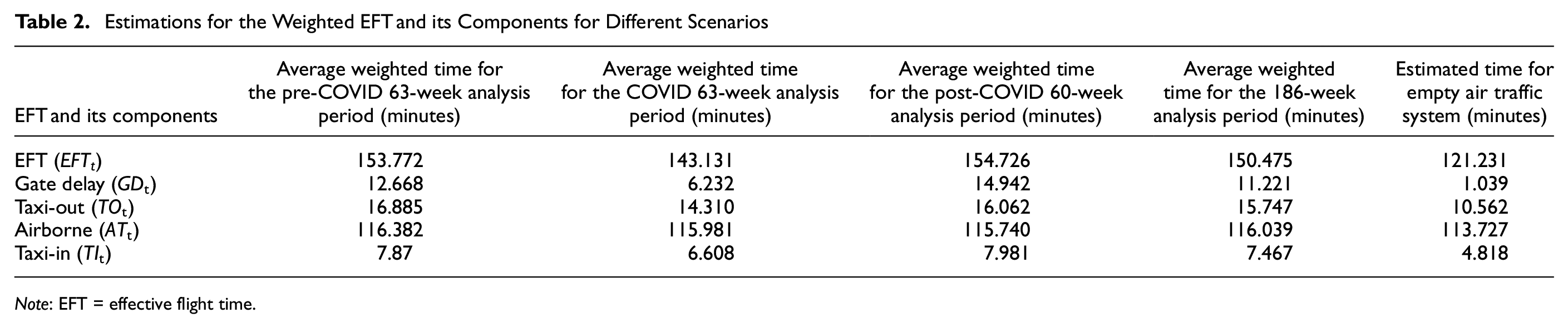
Note: EFT = effective flight time.
For the weighted EFT, the estimation result is 121.231 min. It indicates that the necessary weighted EFT is 121.231 min for an empty air traffic system. The average weighted EFT is 150.475 min for the 186-week analysis period, which means that 25% more weighted EFT time is caused in some way by the presence of other flight traffic. This increase is mainly from gate delay, whose actual average value is 10 min more than for the empty system, in which it essentially disappears. The residual gate delay in the empty system is presumably the result of delays in loading aircraft as well as known and expected delays. A busy air traffic system also has an impact on taxi times. Both taxi-out and taxi-in times increased around 50% compared with the empty scenario. This may be explained by queues for flights about to depart and queues at the destination gate. Airborne time is only 2.312 min less in the existing system compared with the empty one. This verifies previous analysis that the total number of flights and airport conditions have little impact on airborne time.
Post-COVID Recovery Performance
The semi-log-linear models perform well on the training set for modeling the relationship between the weighted EFT (as well as its components) and the total number of flights. In this section, we evaluate the model performance in relation to both the training and test set to assess out-of-sample performance of the trained model and to identify changes in operational performance in the post-COVID period. The test period is from June 1, 2021 to July 25, 2022.
Based on Equation 8 and the estimated parameters in Table 1, we calculate the prediction values for the log-transformed weighted EFT and its components. From this we find the root mean square error (RMSE) and the average difference between the predicted and actual values of the dependent variable. As shown in Figure 7, the ground truths and predictions are tracked closely in the training set but are more divergent in the test set. Figure 8 reveals that the residuals are evenly distributed around 0 in the training set, whereas there are systematic biases in the test set. These differences are confirmed in Table 3, which shows that the RMSEs are larger for the test set, and that the average residuals are non-zero. These average residuals suggest how performance during the post-COVID recovery period has changed. They imply that overall EFT is about 3% greater than what is predicted by a model trained on pre-recovery data. However, we see larger differences in certain EFT components. Specifically, gate delay is about (exp(.393)-1)*100 = 48% greater and taxi-in time is about (exp(.065)-1)*100 = 6.7% greater, whereas changes in airborne time (+0.8%) and taxi-out time (-0.2%) are minimal.
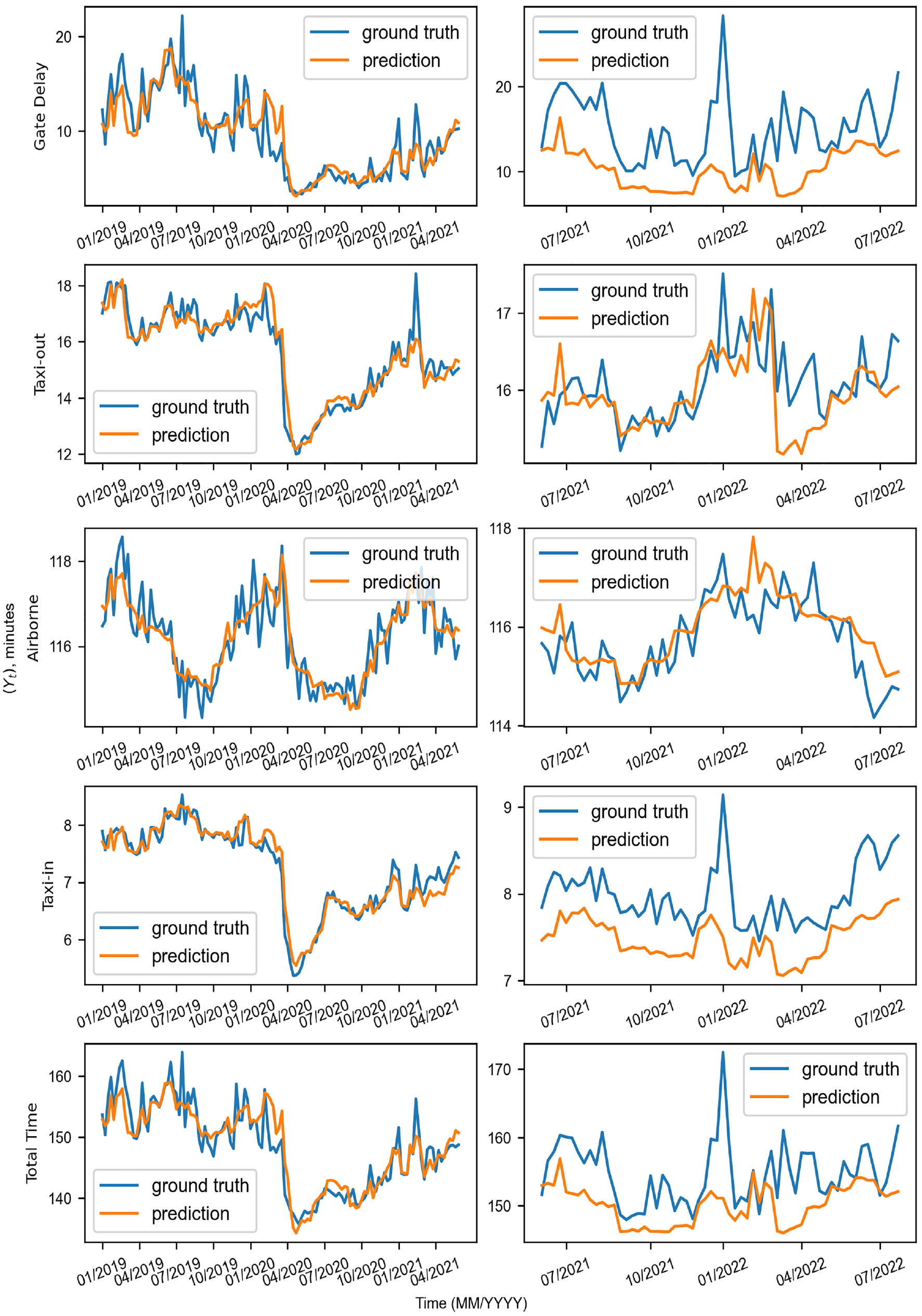
Ground truths and predictions for both training and test sets.
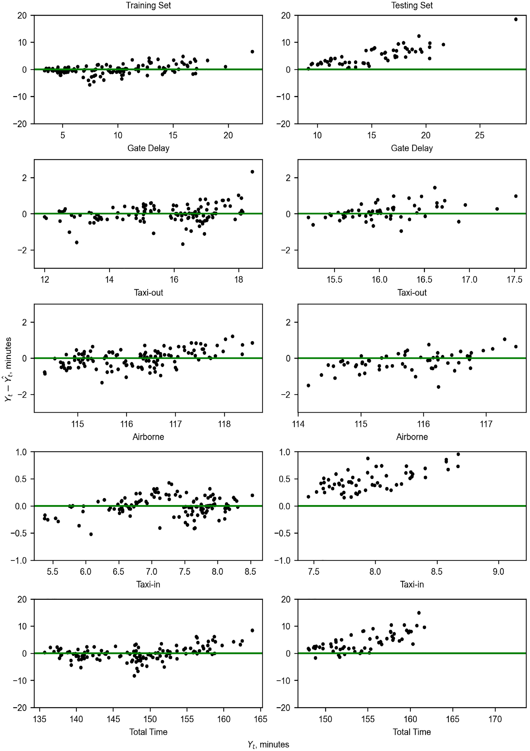
Residuals for both training and test sets.
Prediction Performances of the Training and Test Sets
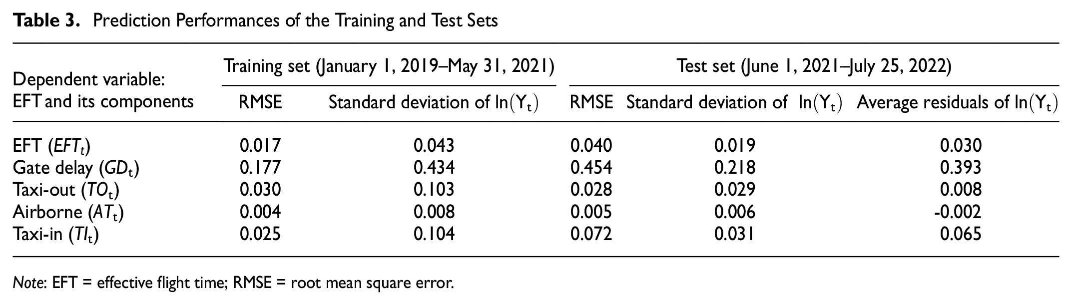
Note: EFT = effective flight time; RMSE = root mean square error.
These results suggest that the perceived degradation in operational performance in recent months is partly illusory and partly real. The EFT has increased, but this is largely to be expected as a result of increased traffic in the system. Nonetheless, EFT is about 3% greater than might be expected based on an increase in traffic alone. Moreover, certain EFT components, namely, gate delay and taxi-in time, have shown more substantial percentage increases. One possible reason is labor shortages, which inhibit the ability of airlines to achieve timely departures or expeditiously move landed aircraft to their arrival gates. Delays resulting from these problems are more evident to the traveling public, even if the change in EFT is fairly small.
Conclusion and Future Work
In this paper, we utilize the natural experiment provided by the COVID-19 pandemic, which caused dramatic fluctuations in air traffic, to quantify the relationship between flight volume and the operational performance of the flight system. Analysis of changes in operational performance allows us to investigate to what extent delays can be explained by a high volume of traffic and whether there are other factors leading to a high level of delays in the post-pandemic world. We develop regression models to formalize this relationship and compare the operational performance between the pre-pandemic and post-pandemic periods by incorporating flight volume as a predictor to reveal if there are any changes. A flight basket for the U.S. domestic aviation market is constructed based on the FAA ASPM database for the analysis period, that is, from January 1, 2019 to July 25, 2022. We first determine the airport OD pairs that should be included in the flight basket, and assign weights to each airport pair based on the number of flights performed over the analysis period. To understand the relationship between air traffic and operational performance further, semi-log-linear models are formulated and estimated using the training dataset from January 1, 2019 to May 31, 2021. We include the primary variable of interest (the total number of flights) in the model, as well as metrics based on fluctuations in airport demand-to-capacity ratios and monthly dummy variables to capture the potential effects of other factors. The model captures a statistically significant positive relationship between EFT and the total number of flights. The estimation results suggest that flight times in a system with zero traffic would be about 30 min less than one with the levels of traffic observed in 2019, with most of the differences in the gate delay and taxi-out segments. Using the estimated coefficients, we test the model on the unseen test period (i.e., post-recovery period), from June 1, 2021 to July 25, 2022. Our models have a good performance with regard to the training set, and similar but not identical results in relation to the test set, for which RMSEs are slightly larger and residuals have systematic biases for certain EFT components. The positive residuals for gate delay and taxi-in time during the test period indicate that certain changes in operational performance in the post-pandemic period, for example, increased gate delay, cannot simply be explained by the recovery of flight volume. On the other hand, overall EFT in the post-pandemic period is about 3% greater than what is predicted by the model trained on pre-recovery data.
In future work, we would consider adding more factors that may influence the operational performance of flights to make the model more reliable. It is possible that model performance could be improved by adding more data and relevant features such as queuing delays, convective weather, and wind, as did our other works for modeling system delays ( 7 ). Furthermore, analysis at a micro level may provide more practical insights and help improve the operational performance of the aviation system. This analysis can also be extended to investigate the performance at a single airport or for a specific group of flights.
Footnotes
Author Contributions
The authors confirm contribution to the paper as follows: study conception and design: J. Xu, L. Dai, M. Hansen; data collection: J. Xu, L. Dai; analysis and interpretation of results: J. Xu, L. Dai, M. Hansen; draft manuscript preparation: J. Xu, L. Dai, M. Hansen. All authors reviewed the results and approved the final version of the manuscript.
Declaration of Conflicting Interests
The author(s) declared no potential conflicts of interest with respect to the research, authorship, and/or publication of this article.
Funding
The author(s) received no financial support for the research, authorship, and/or publication of this article.