Sage Journals: Discover world-class research

Abstract

Providing real-time crowding information in urban railways would enable informed travel decisions and encourage cooperative behavior of passengers, as well as improve operating efficiency and safety. However, the problem of real-time crowding prediction is not trivial because of the unavailability of ground-truth crowding data, particularly for the direct impact of crowding on passengers (e.g., denied boarding on platforms). This paper proposes a data-driven method for real-time denied boarding prediction in urban railway systems using automated fare collection (AFC) and automated vehicle location (AVL) data. It predicts the denied boarding probability distribution or its derived metrics as a function of explanatory variables, including demand, operations, and incident-related factors. The method is validated through a case study covering 18 months on Hong Kong Mass Transit Railways. The results highlight the model’s accurate and robust performance in predicting denied boarding on platforms using purely AFC and AVL data (e.g., an average of 6%–7% error) under both recurrent and non-recurrent situations, in which transfer demand-related factors contribute most to the prediction. The prediction model outputs can support proactive operations control and management, as well as provision of customer information without relying on expensive and time-consuming data collection efforts. Customer information, for example, can include the average number of trains to wait before boarding or the average waiting time on the platform.

Keywords

rail transit systems crowding prediction denied boarding probability big data smart card data

Increases in ridership are outpacing capacity in many large urban rail transit systems, such as Hong Kong’s Mass Transit Railway (MTR), the London Underground, and the New York subway system ( 1 , 2 ). Crowding at stations and on trains may affect safety, service quality, and operating efficiency. Various studies have measured passengers’ willingness to pay for less crowded conditions ( 3 ) and suggested incorporating the crowding disutility in investment appraisals ( 4 ). Furthermore, safety concerns related to crowding are more prevalent following the advent of COVID-19. The pandemic emphasized the requirement of reliable crowding management strategies in urban rail systems.

Congestion management in traffic has been studied extensively including the effectiveness of various strategies such as traffic control, ramp metering, and congestion pricing ( 5 , 6 ). On the other hand, crowd management in transit is still evolving. Adding capacity (e.g., building new lines and shortening headways) to deal with the increased demand is often difficult, especially in the short term. Transit demand management (TDM) strategy for better utilization of available capacity is a promising alternative to deal with this challenging issue. Many agencies have implemented or tested TDM strategies in transit systems, which usually take the form of incentives and penalties ( 7 ). In addition, TDM also includes approaches like directing passengers on the platform to less crowded doors to even the train load. With the prevalence of advanced technologies in automated data collection in transit systems, such as automatic fare collection (AFC) and automatic vehicle location (AVL), many cities have been providing real-time information at stations, on websites, or in mobile applications. Survey results show that around 70% of transit operators are now offering certain levels of real-time information ( 8 ) and that real-time information improves passenger’s perceived service quality ( 9 , 10 ), which has great potential for crowding management.

From the point of view of customer information provision, although different types of information are provided by transit agencies, real-time crowding information on trains or platforms is not common. The problem of real-time crowding prediction is not trivial because of the unavailability of ground-truth crowding data, particularly for the direct impact of crowding on passengers (e.g., denied boarding probabilities on platforms). Standard ways for crowding data collection include manual counting or video processing, which cost time and resources and are prone to human errors. Because of the lack of such data, training models to predict crowding has not been possible Therefore, prediction of real-time crowding from the passengers’ perspective using only AFC and AVL data has not been addressed in the literature, and presents an important research gap.

From the point of view of prediction, many prediction approaches (statistical, machine learning, and deep learning based) have been proposed for a wide spectrum of transportation applications, such as travel times, demand, operation delays, individual mobility, and in-vehicle crowding ( 11 – 13 ). However, no study was found to predict the denied boarding probabilities (i.e., the direct impact of system crowding on passengers) in public transport systems. The distribution of the number of times a passenger is denied boarding because of crowding provides the most detailed and useful performance metric for on-platform crowding and it also allows for the calculation of intuitive performance metrics, such as average waiting time on the platform or the number of trains to wait before boarding a train.

To bridge these gaps, this paper proposes a data-driven crowding prediction method from passengers’ perspective (i.e., denied boarding probabilities and average waiting time on platforms) in urban rail systems using purely automated collection data. It also develops typical machine learning prediction models to explore important variables and model characteristics useful for deployment in practice. The proposed method uses the structure mixture model of Ma et al. ( 11 ) to estimate historical denied boarding distributions using AFC and AVL data, and then formulates supervised learning models to predict the real-time crowding situation on platforms in real time. The key contributions are:

Propose a real-time data-driven prediction framework for crowding in urban railways using AFC and AVL data that enables proactive traffic management and travel recommendations;

Develop machine learning models to predict the crowding from passengers’ perspective, for denied boarding probabilities and average waiting times on platforms;

Validate the model performance using data from the Hong Kong MTR and explore important variables and model characteristics.

The rest of the paper is organized as follows. The “Literature Review” section provides a literature review of crowding management studies (incentives, planning, and real-time information). “Methodology” develops the crowding prediction framework and formulates the supervised crowding prediction problem together with explanatory variables. “Case Study” validates the model performance and explores important factors in driving predictions. The final section summarizes the main conclusions and future work.

Literature Review

Crowding management is implemented in many different forms in various transit agencies. One way is by providing incentives for passengers. Some examples include free fares to incentivize pre-peak travel in Melbourne and Singapore ( 12 , 13 ) or route-based discounts tried in Hong Kong ( 14 ). Applications of off-peak discounts and peak surcharges have been implemented in cities like London, Tokyo, Sydney, and Washington D.C. ( 15 ). Other examples include working with employers to encourage company-specific programs in Singapore ( 16 ) and lottery rebate programs such as San Francisco’s PERKS program ( 17 ). Empirical research on the effectiveness of incentive strategies shows that 2%–5% of passengers shift their travel behavior in response to various incentives ( 18 ). Similarly, San Francisco’s PERKS program resulted in a 10% shift from peak-time travel. Empirical studies reported factors affecting behavior change, such as flexibility, demographics, trip length, and discounts ( 18 , 19 ).

Some studies have considered tactical planning methods to alleviate certain bottlenecks in the system that result in crowding. This kind of planning aims to induce behavior change in passengers in ways other than direct incentives. There is empirical evidence that people’s travel behavior is affected by attributes that are usually ignored in the literature, such as directness of the route and the passenger’s path within a station ( 20 ). Following this, Muñoz et al. ( 21 ) proposed a methodology using one-way gates on platforms to control passenger car boarding choices. Similarly, optimizing the train stop position considering passenger distribution on platforms and station entries is proposed to reduce the uneven distribution of passenger loads on trains ( 22 ).

The availability of automated data sources like AFC and AVL is the enabler for developing crowding estimation and prediction methods, while the prevalence of smartphones facilitates the delivery of related information to users in real time. This dissemination of information provides the opportunity to incite cooperative behavior from passengers while they make informed travel decisions. Moreover, real-time information has the potential to incite long-term changes in travel behavior as many studies have shown the value of real-time information on passengers’ perceptions of waiting times, safety and security, impacts of service disruptions, and general satisfaction ( 7 , 10 , 23 , 24 ). There are many studies focusing on prediction of bus arrival time using various data sources like Wi-Fi ( 25 ) and models like support vector machine (SVM) ( 26 ) and artificial neural networks (ANN) ( 27 , 28 ). For urban railway operations, real-time vehicle location information is shown to benefit service quality as well ( 29 ). There is also research focusing on the prediction of real-time train arrival times to reduce workload for operators ( 30 ).

Very few studies have focused on real-time information directly related to crowding. The value of providing real-time crowding information is shown through a case study in Stockholm where the real-time information is shown to reduce crowding in trains by 4.3% ( 31 ). Existing crowding prediction methods focus on the in-vehicle load prediction using directly observed counts or load data, such as prediction of train load using train assignment models ( 32 , 33 ), prediction of bus load using smart card data ( 34 ), and the car-specific train load information using train weighting data ( 35 ) or hybrid simulation and demand prediction models ( 36 ). However, the real-time prediction of crowding from passengers’ perspective (i.e., denied boarding on platforms) has not been reported in the literature, which is important for proactive demand management and travel planning. This paper bridges this gap by proposing a data-driven crowding prediction framework in urban railways using AFC and AVL data and developing typical prediction methods to identify important predictors and explore model characteristics.

Methodology

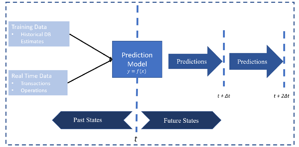
Figure 1 shows the proposed data-driven crowding prediction framework. The time is divided into discrete time intervals of length $Δ t$ (e.g., 15 min). The prediction takes place in these discrete time intervals. At time $t$ , the problem becomes predicting the value of the response variable for the time interval $[t, t + Δ t]$ using observed (recent) AFC (passenger activity) and AVL (train movement) information. Using past denied boarding information allows us to predict crowding from passengers’ perspectives without relying on direct observations.

Figure 1.

Framework of the crowding prediction methodology. The historical denied boarding (DB) estimates are used as the training data. Recent automated fare collection (AFC) transactions and train operations-related information are used to provide real-time predictions on a rolling horizon.

The method uses the structured Gaussian mixture model (GMM) from Ma et al. ( 11 ) to generate the training data (historical DB) for the real-time crowding prediction. The structured GMM estimates the probability distribution of the number of times passengers are denied boarding on a platform in a given discrete time interval, and its performance was validated against survey results in Hong Kong. Various performance metrics for crowding can be derived from the denied boarding probabilities, such as denied boarding rate ( $DBR$ , percentage of passengers not being able to board the first train on their arrival at the platform), expected number of trains to wait $(E (N))$ , and expected waiting time $(E (t^{w}))$ .

The framework utilizes historical denied boarding estimates instead of direct crowding observations (e.g., counts). Therefore, the crowding prediction problem becomes a supervised learning problem in which the denied boarding estimates serve as the response variable. Various station and operations-related features, such as demand and headways, serve as the predictor variables which are used to extract the useful relationships and historical patterns required for predictions. To develop a pure data-driven prediction model, the predictor variables are selected as those directly extracted or estimated from AFC and AVL data.

The data-driven crowding prediction model has three main steps: (i) selection of the feature variables, (ii) selection of the response variables, and (3) development of the prediction model. The feature variable selection involves identifying a set of explanatory variables for the prediction problem. The feature selection enables gaining insights into the impact of factors on crowding. Similarly, the response variable selection involves identifying which measure to use as the indicator for crowding. Since denied boarding probabilities are used, it is possible to derive multiple performance metrics for crowding which can be used as response variables. The model development step involves selecting the supervised learning model and training its parameters to achieve the best prediction accuracy.

Feature Variable Selection

The explanatory variables considered are broadly categorized into three groups: (i) demand-related, (ii) operations-related, and (iii) incident-related features. Note that all the explanatory variables are system attributes known and directly observable from AFC and AVL data in (almost) real time. Demand, operations, and incident-related features are used to capture deviations from regular operations. Variables indicating disruptions are also included, since incidents in the system may have a large impact on crowding levels. Table 1 provides the overview of the used predictor variables.

Table 1.

Overview of the Feature Variables and Their Notations

Demand	Operations	Incident
Station demand $(D_{s, t})$	Average headway $({\bar{H}}_{s, t})$	Accumulation $(A (t))$
Upstream demands $(D_{s, t}^{up})$	Number of trains $(N_{t})$
	Station left-over demand $(L_{s, t})$
	Upstream left-over demand $(L_{s, t}^{up})$

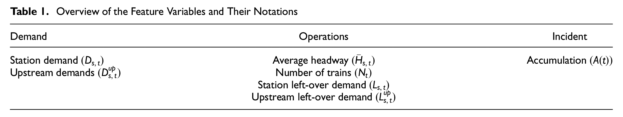
Demand

Demand-related features involve real-time AFC transactions from passengers entering the station of interest and upstream stations. Upstream stations are those belonging to the same line as the studied station as well as transferring lines connecting to the station in the same direction. For same-line stations, upstream demand serves as an indicator of used capacity. The higher the demand in upstream stations, the higher the train load when the train arrives at the platform. This, in turn, will result in a higher probability of denied boarding and higher crowding levels at the current platform. Also, upstream stations from connecting lines are considered proxies for transfer demand. Higher transfer demand is also expected to result in higher crowding at transfer stations.

The upstream demands can be included in the model either as aggregate or disaggregate features. If they are included as aggregate features, each upstream branch is represented as a single feature variable by summing up individual station demand along that branch. On the other hand, if disaggregate features are used, each upstream station is represented as a separate explanatory variable. The disaggregate features may generate a high number of explanatory variables, which may affect the model’s predictive accuracy. The variability between stations could be lost if aggregate features are used. Both versions are tested in the case study to assess the impact of aggregate/disaggregate demand features on crowding prediction.

Operations

For the operations-related features, the aim is to identify a set of variables that are able to capture current system performance. The average headway and the number of trains arriving at the platform (both from the same and transferring lines) in the current time interval $([t - Δ t, t])$ are used to capture the current service level. The number of trains is also used because the average headway by itself is not enough to indicate the level of service. Given a time interval $[t, t + Δ t]$ , the average headway might be very low for a few trains arriving on the platform as well. However, if the number of trains arriving at the platform during $[t, t + Δ t]$ is also small, it is not considered a good service. It is expected that a lower average headway value and a higher number of arriving trains are associated with a decreased crowding situation on platforms.

In addition, a set of feature variables, referred to as left-over demand, is used to capture the amount of demand that could not be served in the last time interval and carried over to the next time interval. The left-over demand is calculated both for the station of interest and for upstream stations:

L_{s, t} = A_{s, t} \times τ

(1)

L_{s, t}^{up} = A_{s, t}^{up} \times H_{last}

(2)

where $L_{s, t}$ and $L_{s, t}^{up}$ are the left-over demands for the station of interest and the upstream stations, $A_{s, t}$ and $A_{s, t}^{up}$ are the average passenger arrival rates for the station of interest and the upstream stations, $H_{last}$ is the headway of the last train arriving from the transfer line and $τ$ is the time between the arrival of the last train and the beginning of the new prediction interval.

Figure 2 illustrates the arrival times of trains from both the main and transferring lines at the station of interest. $L_{s, t}^{up}$ represents the number of passengers transferring to the station of interest with the latest train that has arrived at the station. These passengers have the highest probability of being carried over to the next time interval. Similarly, $L_{s, t}$ captures the number of passengers arriving at the platform after the last train from the same line left the platform. Note that the left-over demands and the average arrival rates are time-specific and calculated separately for each time interval. These passengers tapping in at the station of interest are the passengers who will be added to the demand of the next time interval. It is expected that higher left-over demands (for both upstream and station of interest) are associated with higher platform crowding.

Figure 2.

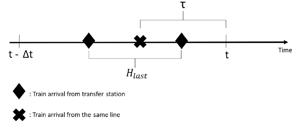
Train arrival times at the platform for the calculation of left-over demands.

Incidents

Known incidents in the system are considered within the prediction framework since they are expected to influence system crowding. We used a predictor variable, namely the accumulation of demand in the system ( 37 ), to approximate the impact of the incident at a system level. The accumulation at time $t$ , $A (t)$ is defined as the total number of passengers inside the system:

A (t) = \int_{0}^{t} a (t) dt - \int_{0}^{t} e (t) dt

(3)

where $A (t)$ is the accumulation at time $t$ , $a (t)$ is the arrival rate of passengers (at all stations in the system) at time $t$ , and $e (t)$ is the exit rate of passengers at all stations in the system.

The accumulation of demand can be calculated from passengers’ entry and exit AFC transactions. The accumulation of passengers in the system is expected to increase under serious disruptions since the railway system may take longer to move passengers and operate under reduced throughput. The impact of such a disruption would not be reflected necessarily in station demand features as these only count the people entering the system. Similarly, the operations-related features would only reflect an incident if it happens at the same line. The accumulation of demand variables adds a system-level indicator to the feature set. It also incorporates the exit rate from the system which enables tracking the system-wide impacts of disruptions.

Response Variables

We consider two different approaches for the response variable for the prediction problem. Firstly, we consider the problem of predicting the entire vector of denied boarding probabilities. This corresponds to a multi-dimensional response variable where $Y$ is a vector of size $| N |$ and each component $y_{n}$ represents the probability of denied boarding $n \in {0, \dots, N}$ times. Since the response variable $y$ represents a discrete probability distribution, the prediction needs to satisfy two conditions: $0 \leq y_{n} \leq 1 \forall n \in {0, \dots, N}$ ; and $\sum_{n} y_{n} = 1$ . Therefore, the denied boarding probability prediction problem is formulated as a classification problem.

We also consider a one-dimensional version that uses either the denied boarding rate $(DBR)$ or the expected waiting time $(E (w))$ as the response variable. Such measures can be easily derived from the denied boarding probabilities in the training set. Both response variables are practical and easy to interpret as opposed to $E (N)$ which may be useful for planning purposes but may not be very informative for communicating to passengers. In the one-dimensional prediction problem, the denied boarding probabilities are converted to the corresponding response variable and the problem becomes a typical regression problem.

The denied boarding rate in a time interval refers to the probability that a passenger will experience denied boarding at least once during that time interval. It is calculated as:

DBR = 1 - P (NoDeniedBoarding) = 1 - P_{0}

(4)

where $P_{0}$ is the probability of experiencing no denied boarding (i.e., boarding the first arriving train).

The expected waiting time for a passenger in a time interval is calculated using the denied boarding probabilities and the average headway within the time interval:

E (w) = \sum_{n = 1}^{N} (\frac{\bar{H}}{2} + n * \bar{H}) * P_{n}

(5)

where $\bar{H}$ refers to the average headway and $P_{n}$ refers to the probability of being denied boarding $n$ times.

Even though variables $DBR$ and $E (w)$ convey useful information about crowding, $E (w)$ is more representative of the whole denied boarding probability distribution and of interest to passengers, whereas $DBR$ provides more compressed information. This may cause issues, especially in situations where there are high probabilities of being denied boarding multiple times. For example, consider two scenarios: a scenario where the probability of denied boarding once is equal to one and another scenario where the probability of denied boarding twice is equal to one. Both scenarios would have a denied boarding rate equal to one, although they represent very different situations from the point of view of passenger experience. Thus, $DBR$ does not capture the difference between these two cases whereas the difference would be represented by the $E (t^{w})$ . For the one-dimensional crowding prediction problem, the paper focuses on the expected waiting time predictions.

Prediction Model

The proposed prediction methodology allows the crowding prediction problem to be formulated as a typical supervised learning problem. The model selection step for the supervised learning problem involves selecting a model that best suits the needs and structure of the data set and fine-tuning the parameters to gain optimal results on accuracy and robustness. The expected waiting time and denied boarding probability models are developed separately given that they have different problem characteristics.

The expected waiting time prediction problem is a regression problem in which the aim is to predict one continuous response variable as a function of a set of explanatory variables. Note that the response variable for the time interval $[t, t + Δ t]$ is represented using the explanatory variables observed in previous time intervals. With this formulation, any generic supervised learning algorithm can be used for prediction. Three machine learning models, namely, gradient boosting trees (XGB), random forest (RF), and SVM are considered for the expected waiting time prediction problem. These models are selected because they are efficient and have shown good performance with a high number of explanatory variables. Also, they can be used for regression problems with non-linear decision boundaries capturing complex patterns. Another factor in the model selection is that their outputs provide information about the explanatory powers of the various variables ( 38 – 40 ). Discovering the important features that have the most impact on platform crowding prediction is also a desired output of the model. The three selected methods all have built-in feature importance metrics which can provide such information.

For the denied boarding probability prediction problem, we use a neural network formulation, in which the architecture consists of dense layers and a softmax layer. The model is trained using the categorical cross-entropy loss function to accommodate the prediction of a probability distribution. The softmax function converts a given vector to probabilities that satisfy the requirements for the denied boarding distribution prediction.

For the expected waiting time prediction models, the accuracy is assessed using the mean squared error (MSE), mean absolute error (MAE), and mean absolute percentage error (MAPE) as performance metrics.

MAPE = \frac{1}{n} \sum_{i = 1}^{n} | \frac{y_{i} - {\hat{y}}_{i}}{y_{i}} |

(6)

MAE = \sum_{i = 1}^{n} \frac{| y_{i} - {\hat{y}}_{i} |}{n}

(7)

MSE = \sum_{i = 1}^{n} \frac{{(y_{i} - {\hat{y}}_{i})}^{2}}{n}

(8)

where $n$ is the number of observations and $y_{i}$ and ${\hat{y}}_{i}$ are the actual and predicted values for observation $i$ respectively.

For the denied boarding probability prediction model, we use the Kullback–Leibler (KL) divergence $(D_{KL})$ to assess its accuracy. It calculates the relative entropy from a discrete probability distribution $Q$ to another discrete probability distribution $P$ over the same probability space $N$ .

D_{KL} (P | | Q) = \sum_{n \in N} P (n) \log (\frac{P (n)}{Q (n)})

(9)

The hyperparameters of all models (both expected waiting time and denied boarding prediction models) are optimized using a grid search considering different combinations of parameters. For both the expected waiting time prediction and denied boarding probability prediction models, we use leave-one-out cross-validation for every parameter set within the hyperparameter grid.

Case Study

The case study applies the proposed prediction framework using actual data from the MTR operating in Hong Kong. MTR operates the urban railway transit network serving the urbanized areas in Hong Kong Island, Kowloon, and the New Territories. Currently, the MTR network consists of 11 lines, serving 159 stations (91 heavy rail and 68 light rail stations) with 218.2 km of rail. MTR uses a smart card fare collection system called Octopus which records more than 5 million trips on an average weekday. For the heavy rail lines, the AFC system records both entry and exit transactions which allow for a complete record of each trip.

The denied boarding estimation model in Ma et al. ( 11 ) is used to generate the historical denied boarding data. The prediction model is validated at one key station within the network. The selected platform is one of the busiest platforms in the entire network. In addition to its own demand (highest in the network), it is at the intersection of three lines and receives transfer passengers from three directions. Figure 3 illustrates the network and the studied stations in the case study. The denied boarding model used to generate the training set was validated against manual observations collected at the same platform ( 11 ).

Figure 3.

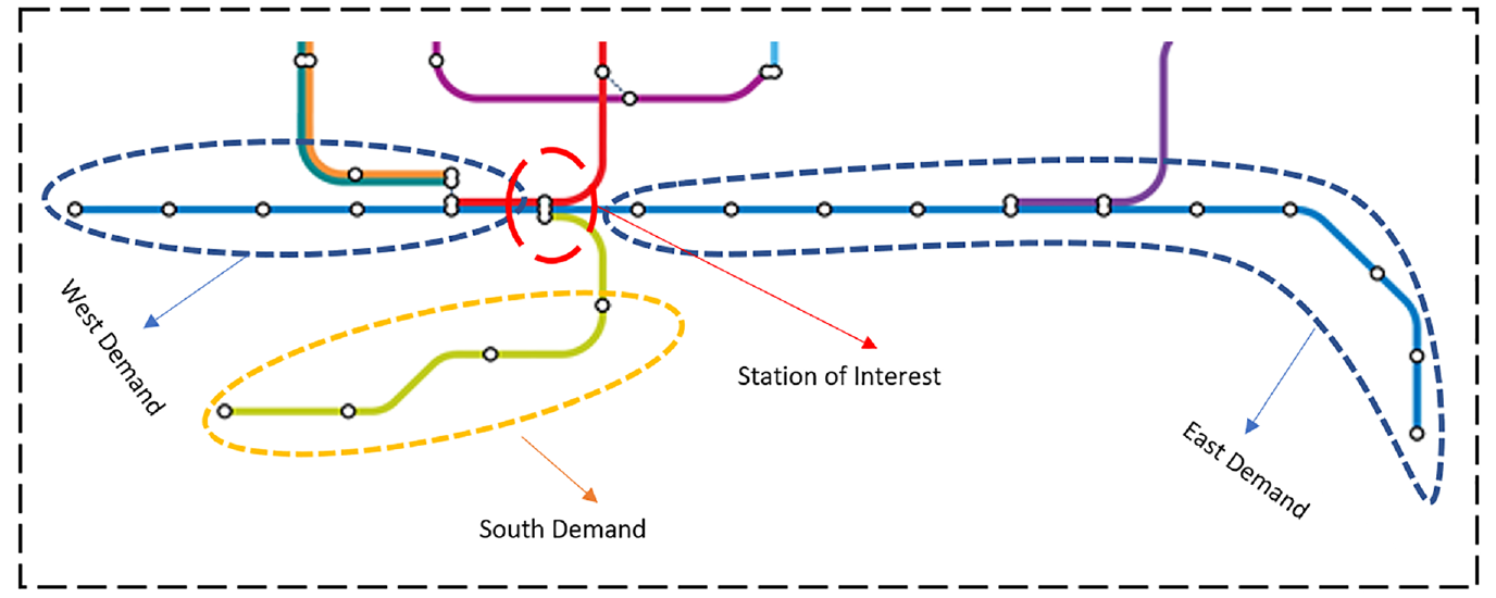
Network used in the case study. The station within the red circle is the station of interest. The three upstream lines are differentiated based on their direction (west, east, south). Both disaggregate and aggregate upstream demands are tested.

The available data covers a period spanning from January 2017 to July 2018. Denied boarding probabilities are estimated in discrete time intervals of 15 min for the evening peak (6:00 to 8:00 p.m.). After removing abnormal days, 295 days are fully processed resulting in 2,360 observations that can be used to train and test the prediction model. The observations that are considered outliers and removed from the dataset had: (a) missing train records in the AVL data (i.e., some trains are on the schedule but are not recorded on the AVL data) and/or (b) incorrect AVL records (i.e., train arrival time for a forward station is before the earlier station, etc.).

The expected waiting time is calculated for all observations from the denied boarding probabilities using Equation 5. The demand and headway-related explanatory variables are calculated for the station of interest and the transfer stations. As shown in Figure 3, the upstream stations are separated into three parts: west, east, and south representing incoming demand and trains from different directions. Both aggregate and disaggregate versions of upstream demand are used. Figure 4 shows the average weekday demand in 15 min time intervals for the station of interest as well as the upstream components (aggregated). It indicates that the majority of transfer demand is generated in the east and west sections (Figure 3). Figure 4 also indicates that the peak of the peak is between 6:00 p.m. and 7:00 p.m. with a gradual decline in demand after 7:00 p.m. The aggregate version consists of three upstream demand features for east, west, and south. On the other hand, the disaggregate version consists of 20 different features representing each upstream station. This results in 11 total features for the aggregate version and 27 for the disaggregate version. Both versions are used for model development and comparison purposes.

Figure 4.

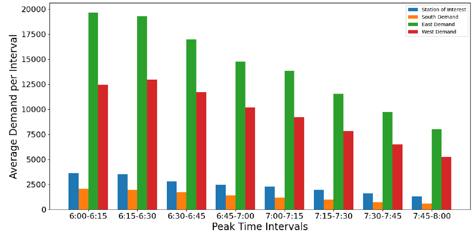
Average weekday demand for a 15 min time interval between 6:00 and 7:00 p.m. for various demand components used in the model.

Parameter Settings

We perform a hyperparameter grid search for both expected waiting time and denied boarding probability prediction models. We have a sample of observations $i \in {1, \dots, n}$ , and a set of supervised learning models $M \in [SVM, RF, XGB, DNN]$ each with a unique parameter grid $M \in M$ . For each $M \in M$ , we consider all potential parameter vectors $X_{k} \forall k \in M$ . For each $X_{k}$ , we perform a leave-one-out cross-validation to acquire the error term for each observation: $e_{i} = y_{i} - {\hat{y}}_{i} \forall i \in {1, \dots, n}$ . We calculate the various performance metrics $(MSE, MAE, MAPE, D_{KL})$ for $X_{k}$ . The reported accuracy for each $M$ is for the $X_{k}$ minimizing the corresponding metric.

For the expected waiting time prediction formulation, all three models (XGB, RF, and SVM) are trained using the skicit-learn package in Python ( 41 ). For the RF model, around 4,000 parameter combinations of different numbers of trees, maximum tree depths, pruning parameters, and split criteria are considered. Similarly, different values for the number of trees, maximum tree depths, and learning rates are considered for the XGB model resulting in around 2,000 combinations. For the SVM model, around 5,000 combinations are considered based on various kernel functions (including kernel-specific parameters), regularization parameters, and epsilon values. Each combination in the expected waiting time formulation is evaluated using the leave-one-out cross-validation.

For the denied boarding probability prediction model, we use the Keras ( 42 ) package in Python to train the neural networks. Our hyperparameter tuning stage includes a different number of layers (up to six layers), various activation functions for intermediary layers, the number of nodes in each layer, and different values for the number of epochs and batch sizes. The number of parameter combinations is around 14,000 and each combination is evaluated using the leave-one-out cross-validation procedure.

Results from the models are also compared with the historical average prediction model. The historical average model prediction is specific to each day of the week and time interval (e.g., Monday 6:00–6:15 p.m.). The averages are used as a naïve predictor. For the denied boarding probability model, we calculate the historical averages for each denied boarding probability, and for the expected waiting time model we calculate the corresponding $E (w)$ .

Expected Waiting Time Prediction

For the expected waiting time models, the prediction results for various scenarios and models are summarized in Table 2, including results for the naïve model. Generally, all three machine learning based models outperform the historical average (naïve) model significantly. For both aggregate and disaggregate features, the XGB model provides the best results even though the differences are small. The small differences in accuracy for the three models indicate that the performance depends more on selected features rather than the selected machine learning model. Once the parameters are fine-tuned to the set of explanatory features, the additional gain resulting from the best machine learning model is marginal. Interestingly, using the aggregate or disaggregate demand features for the upstream stations makes a marginal difference to accuracy. The XGB model performs better with disaggregate features, while the RF and SVM models perform better with aggregate demand features. Considering these observations, the aggregate demand features alternative is preferable since it requires a less number of predictors. The XGB model is also selected as the model for further analysis since it provides the best performance.

Table 2.

Model Performances: Three Performance Metrics Considered for each Model and Compared with the Naïve Model

	Aggregate features model			Disaggregate features model			Historical average
	SVM	RF	XGB	SVM	RF	XGB	Historical average
Mean squared error	989.92	967.33	940.56	997.33	1,068.67	911.77	5,442.45
Mean absolute error	19.31	19.60	19.10	19.56	20.42	18.65	48.65
Mean absolute percentage error	7.68%	7.85%	7.47%	7.77%	8.08%	7.20%	25.56%

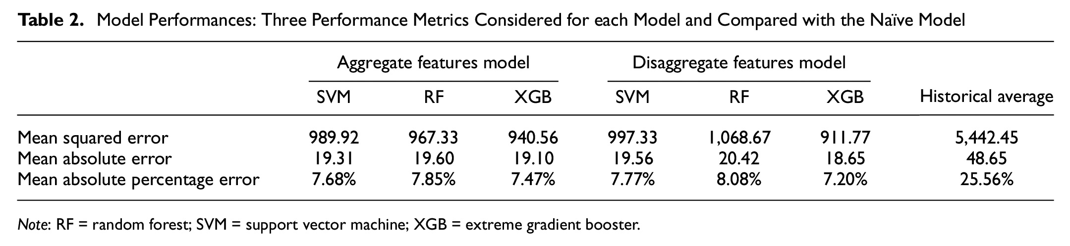
Note: RF = random forest; SVM = support vector machine; XGB = extreme gradient booster.

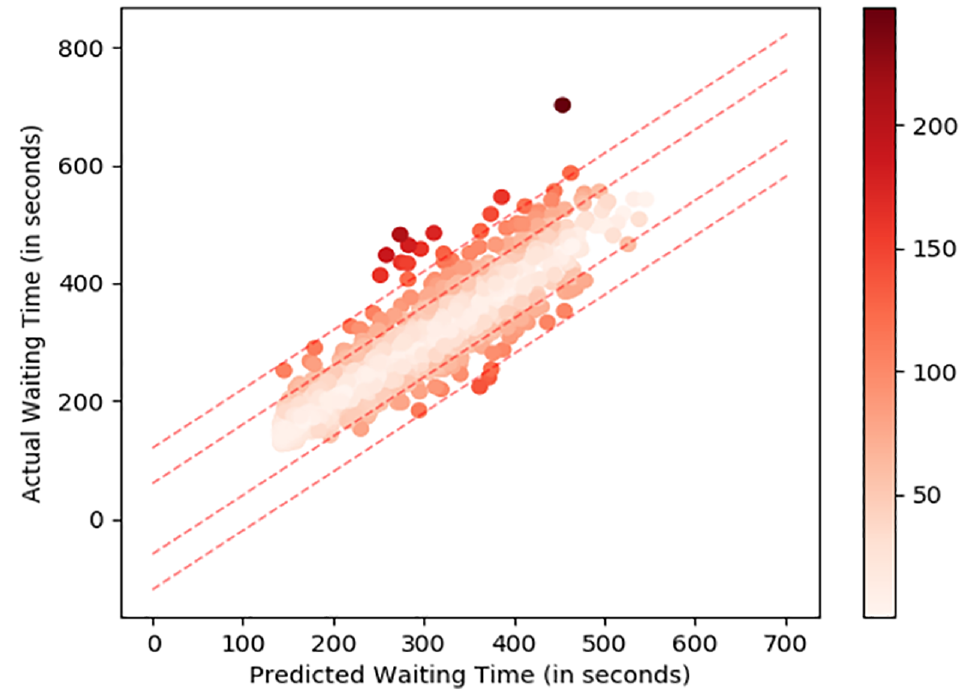
Figure 5 shows the scatter plot of predicted versus the actual values of all observations. Note that the plotted results are reported from the XGB model with optimized parameters. The scatter plot shows that all the observations are distributed around the 45-degree line. The inner dashed lines indicate $\pm 1$ min error and the outer dashed lines indicate $\pm 2$ min error. The MAE for the plotted results is 19.6 s which means that, on average, the predictions are within 20 s of the actual waiting time. This corresponds to around 7% of the average waiting time. Furthermore, it is less than 7% during the peak of the peak (6:00–7:00 p.m.), since the waiting times are higher than the overall average during that period. Moreover, 97% of all predictions are within 1 min of the actual value and 99.25% are within 2 min of the actual waiting time.

Figure 5.

Predicted waiting time against actual waiting time (both in seconds). The inner dashed lines represent 1 min error and the outer dashed lines represent 2 min error. Each observation is color coded where darker colors represent larger errors.

Figure 5 shows that there is a small set of predictions that have errors larger than 3 min. However, it is known that none of the results that have an error higher than 3 min are incident days. In fact, the predictions from the days where there is an incident all have errors smaller than 2 min which suggests that the proposed features are able to capture the effects of incidents. Therefore, the predictions with errors larger than 3 min are either outlier observations of waiting time or cannot be learned by the current set of features. One possible solution to these issues may be using external information such as weather or event information (e.g., a concert) to supplement the existing predictors. Currently, the model only uses explanatory variables that are observable using AFC and AVL data.

Figure 6 shows the distribution of prediction errors from the XGB model with aggregate demand features. The average error by itself might be misleading since the variability in the error is also important. A skewness or bias in the error distribution could imply a methodological error or model bias ( 38 ). The figure shows that the errors are distributed evenly around zero (even close to a normal distribution) with a relatively small variance. The results show that the model predictions are not biased. The low variability shows that the model performs well with all errors distributed close around zero. This supports the results shown in Figure 5. The results show that the predictions that are made using the denied boarding estimates are accurate and robust and can be used for the provision of real-time crowding information in a completely data-driven manner.

Figure 6.

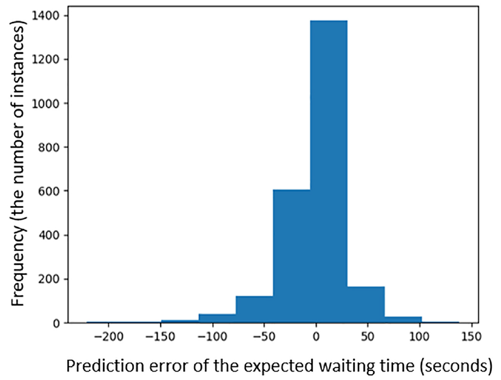
Distribution of prediction errors from the extreme gradient booster model (XGB) with aggregate features.

Feature Importance

The XGB model also outputs the importance of each feature variable. The metric for each predictor is a percentage score that corresponds to the ratio of the gain from the variable to the overall gain. The gain in this context refers to the improvement made in the objective function of the model. Note that, this performance metric is valid only for the XGB model since it is calculated using the splits made in the base learners. Feature importance provides useful insight into the usefulness of the proposed feature set within the XGB model.

Figure 7 shows the feature importance for the XGB model with aggregate demand features. The results show that the transfer demand is the most important factor since east and west demands constitute 90% of the total gain. This is sensible since the demand carried to the station of interest from the parts denoted as east and west are much larger compared with the south demand (reflected in Figure 4). Another reason is using 15 min time intervals. The average waiting time (for a 15 min interval) during the peak of the peak at platform of interest is between 5–6 min. Since the model looks back into the last 15 min period, on average, two-thirds of the passengers tapping in at the station of interest during the past interval would be most probably served. The passengers transferring from other lines would have a delayed impact on crowding. Moreover, the passengers from transferring lines come in bulk and might have a more direct impact on platform crowding. Finally, both the service and the arrival rates in the MTR system are very regular, especially in peak periods. The headway distribution therefore has a low standard deviation and the passenger arrival rate is almost constant. This means that there is low variability in operations-related features such as headways and left-over demands which is another explanation for the high importance associated with transfer demand features.

Figure 7.

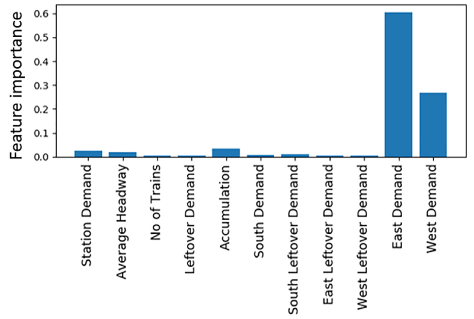
Feature importance for the extreme gradient booster model (XGB) model trained on aggregate demand features.

Based on these observations, another model was built using only the demand-related features to test the impacts on prediction accuracy. The new model resulted in an MAE score of 21.56 s and a MAPE score of 8.43% which shows lower accuracy compared with the original model. This result indicates that, although these variables have low feature importance scores, they still have an impact on the accuracy of the model.

Denied Boarding Probability Prediction

Figures 8 and 9 show the results of the denied boarding probability prediction model compared with historical averages and the actual values over the days with actual observations. Each day shows the average of the corresponding denied boarding probability over the time period between 6 and 7 p.m. This period is selected since the majority of denied boardings occur in this period. Figure 8 shows the results for denied boarding zero times, Figure 9 for denied boarding once, and Figure 10 for denied boarding twice or more. The denied boardings of more than two times are aggregated since the variability for higher denied boarding levels (e.g., 4–5 times) is low and the associated values tend to be close to zero. We observe that the predicted results outperform the model based on historical averages for all three predicted metrics. Moreover, the predicted results are able to capture the fluctuations in denied boarding levels across time.

Figure 8.

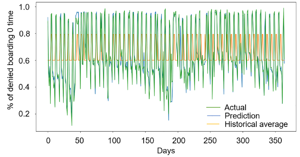
Probability of no denied boarding.

Figure 9.

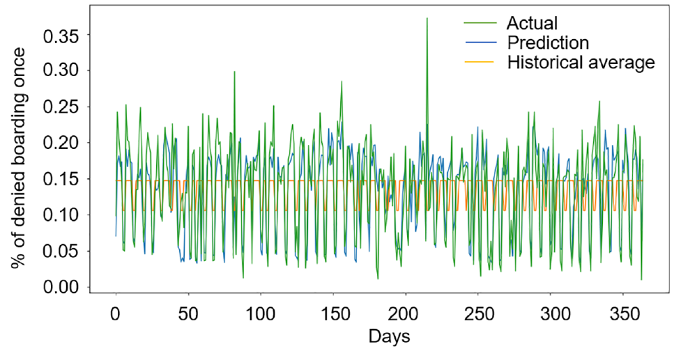
Probability of denied boarding once.

Figure 10.

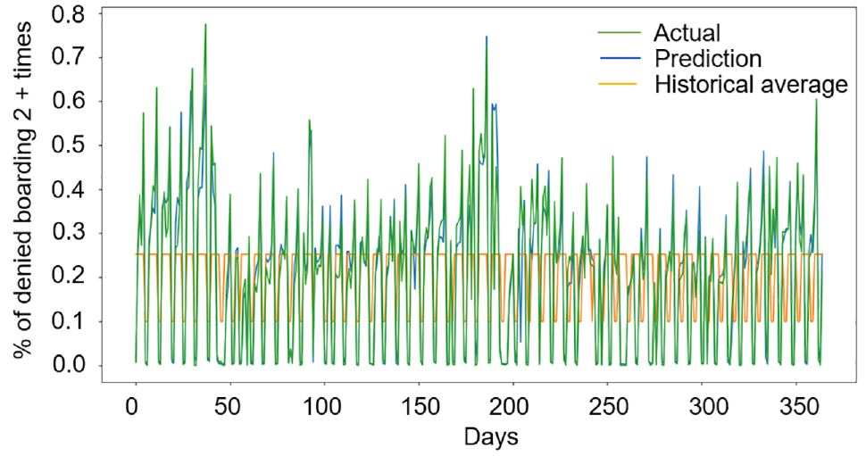
Probability of denied boarding more than twice.

Figure 10 shows that the denied boarding probability prediction model is also able to capture abnormal results in the denied boarding vector. The average waiting time for a weekday between 6:00 and 7:00 p.m. is around 5 min and the average headway for the same interval is around 2 min. This suggests that, on average, passengers are able to board the second train during this 1 h period. Thus, having a high (more than 0.5) probability of denied boarding two or more times can be considered unusual. Our data includes 12 days where the probability of denied boarding twice or more times exceeds 0.5. Figure 10 shows that the predictions are able to capture the majority of these observations. Additionally, the model is also able to capture the days when the probability of denied boarding twice or more exceeds 0.7.

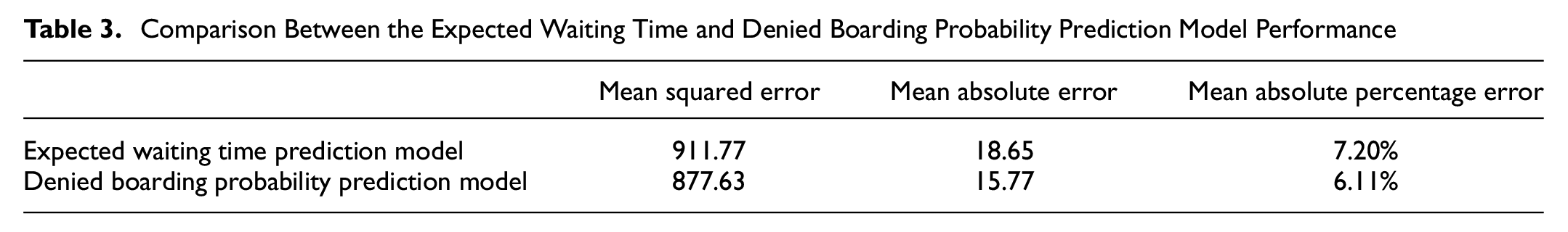
As a further demonstration of the effectiveness of the denied boarding probability prediction approach, we compare the results from the denied boarding probability prediction model with the expected waiting time model predictions. We use the predicted denied boarding vector for every interval and day in the dataset to calculate the corresponding expected waiting time. This provides a basis for comparison by enabling the calculation of MAE, MAPE, and MSE measures related to the average waiting time corresponding to the predictions by the denied boarding probability prediction model. The aggregate metrics (e.g., expected waiting time) are more useful for information dissemination.

Table 3 provides the comparison of results across different accuracy metrics. The MAE, MSE, and MAPE values for the denied boarding probability prediction model are 15.77, 877.63, and 6.11%, respectively. Compared with the expected waiting time prediction approach, we observe around 3 s of decrease in absolute prediction errors and more than 1% decrease in MAPE. Moreover, 93% of all the predictions have errors below 1 min and 99.5% of predictions have errors lower than 2 min compared with higher values for the expected waiting time prediction models. These results indicate that the denied boarding probability prediction model outperforms the best expected waiting time prediction model (XGB). Thus, having a denied boarding probability prediction approach is preferable to an expected waiting time prediction approach. The reason for the improvement in accuracy is that the denied boarding probability prediction model is trained using more detailed data (denied boarding vector), whereas the expected waiting time prediction method is trained on aggregated information (expected waiting time). The higher granularity of information is used in the training and validation of the denied boarding probability prediction model. This enables the model to capture details across the denied boarding vector, thus providing better predictions.

Table 3.

Comparison Between the Expected Waiting Time and Denied Boarding Probability Prediction Model Performance

	Mean squared error	Mean absolute error	Mean absolute percentage error
Expected waiting time prediction model	911.77	18.65	7.20%
Denied boarding probability prediction model	877.63	15.77	6.11%

Conclusion

Real-time crowding prediction is important for operating control and information provision in public transport. However, the problem is not trivial because of the unavailability of ground-truth crowding data. No study was found on predicting the direct impact of crowding on passengers (e.g., denied boarding on platforms). The paper proposes a data-driven method for real-time denied boarding prediction using purely the automatically collected AFC and AVL data in urban railways. Two different prediction problems are formulated, including the expected waiting time and denied boarding probabilities prediction. The historical denied boarding estimates are estimated using a structured GMM from Ma et al. ( 11 ). The demand, operations, and incident-related factors are designed as model predictors which are readily extracted or estimated from AFC and AVL data. Typical machine learning models are developed to explore the importance of predictors and model characteristics.

The prediction method is validated through a case study covering 18 months in the MTR network in Hong Kong by comparing it with historical denied boarding estimates and typical machine learning models. The results show that the XGB model provides the best prediction among expected waiting time prediction models even though the differences are small. The transfer demand predictors contribute mostly to the real-time crowding prediction. The neural networks based denied boarding probability prediction model can accurately predict the denied boarding probability distribution in both regular and irregular conditions (i.e., with incidents) and it also outperforms the best expected waiting time prediction model (i.e., XGB). Overall, the proposed model can provide accurate and robust crowding conditions using purely automated collection data (e.g., the denied boarding probability prediction model has a mean percentage error of 6% with 93% cases within 60 s).

The online denied boarding prediction model can support applications of real-time operation control and management and customer information provision (e.g., the number of trains to wait before boarding a train) without relying on expensive and time-consuming data collection efforts. The method is applicable to closed transit fare systems with both entry and exit ticket validations. For fare systems with only entry ticket validations, the denied boarding probability could be inferred using the transit assignment method with the estimated origin–destination demand matrix and observed crowding on platforms ( 43 ).

Footnotes

Acknowledgements

The authors acknowledge the Mass Transit Railway, Hong Kong for providing the data for the study.

Author Contributions

The authors confirm their contribution to the paper as follows: study conception and design: K. Tuncel, H. Koutsopoulos, Z. Ma; data collection: K. Tuncel, Z. Ma; analysis and interpretation of results: K. Tuncel, H. Koutsopoulos, Z. Ma; draft manuscript preparation: K. Tuncel, Z. Ma. All authors reviewed the results and approved the final version of the manuscript

Declaration of Conflicting Interests

The author(s) declared no potential conflicts of interest with respect to the research, authorship, and/or publication of this article.

Funding

The author(s) received no financial support for the research, authorship, and/or publication of this article.

ORCID iDs

Kerem S. Tuncel

Haris N. Koutsopoulos

Zhenliang Ma

Data Accessibility Statement

The data that support the findings of this study are available from the corresponding author on reasonable request.

References

Zhu

Koutsopoulos

H. N.

Wilson

N. H.

Inferring Left Behind Passengers in Congested Metro Systems From Automated Data. Transportation Research Procedia, Vol. 23, 2017, pp. 362–379.

Zhu

Koutsopoulos

H. N.

Wilson

N. H.

A Probabilistic Passenger-to-Train Assignment Model Based on Automated Data. Transportation Research Part B: Methodological, Vol. 104, 2017, pp. 522–542.

Hensher

D. A.

Crowding and Public Transport: A Review of Willingness to Pay Evidence and its Relevance in Project Appraisal. Transport Policy, Vol. 18, No. 6, 2011, pp. 880–887.

Haywood

Koning

The Distribution of Crowding Costs in Public Transport: New Evidence From Paris. Transportation Research Part A: Policy and Practice, Vol. 77, 2015, pp. 182–201.

Dixit

V. V.

Harb

R. C.

Harrison

G. W.

Marco

D. M.

Mard

Radwan

A. E.

Rutström

Schneider

M. P.

Review of Congestion Pricing Experiences, Federal Highway Administration, 2010.

Kachroo

Gupta

Agarwal

Ozbay

Optimal Control for Congestion Pricing: Theory, Simulation, and Evaluation. IEEE Transactions on Intelligent Transportation Systems, Vol. 18, No. 5, 2016, pp. 1234–1240.

Koutsopoulos

H. N.

Halvorsen

Zhao

Demand Management in Urban Railway Systems: Strategy, Design, Evaluation, Monitoring and Technology. In Handbook of Public Transport Research, Edward Elgar Publishing, Graham Currie, Cheltenham, UK, 2021, pp. 314–339.

Harmony

X. J.

Gayah

V. V.

Evaluation of Real-Time Transit Information Systems: An Information Demand and Supply Approach. International Journal of Transportation Science and Technology, Vol. 6, No. 1, 2017, pp. 86–98.

Burge

Heywood

Sheldon

Lee

Barber

Phillips

The Impact of Real-Time Information on Passengers’ Value of Bus Waiting Time. Transportation Research Procedia, Vol. 31, 2018, pp. 18–34.

10.

Watkins

K. E.

Ferris

Borning

Rutherford

G. S.

Layton

Where Is My Bus? Impact of Mobile Real-Time Information on the Perceived and Actual Wait Time of Transit Riders. Transportation Research Part A: Policy and Practice, Vol. 45, No. 8, 2011, pp. 839–848.

11.

Koutsopoulos

H. N.

Chen

Wilson

N. H.

Estimation of Denied Boarding in Urban Rail Systems: Alternative Formulations and Comparative Analysis. Transportation Research Record: Journal of the Transportation Research Board, 2019. 2673: 0361198119857034.

12.

Currie

Exploring the Impact of the “Free Before 7” Campaign on Reducing Overcrowding on Melbourne’s Trains. 32nd Australasian Transport Research Forum, Vol. 32, Auckland, New Zealand, 2009.

13.

Pluntke

Prabhakar

INSINC: A Platform for Managing Peak Demand in Public Transit. Journeys, Land Transport Authority Academy of Singapore, Vol. 2013, 2013, pp. 31–39.

14.

S.-M.

Wong

F. C.

The Effectiveness of Differential Pricing on Route Choice. Transportation, Vol. 21, No. 3, 1994, pp. 307–324.

15.

Koutsopoulos

H. N.

Noursalehi

Zhu

Transit Data Analytics for Planning, Monitoring, Control, and Information. In Mobility Patterns, Big Data and Transport Analytics ( Antoniou

Dimitriou

Pereira

, eds.), Elsevier, Amsterdam, Netherlands, 2019, pp. 229–261.

16.

Halvorsen

Koutsopoulos

H. N.

Zhao

Demand Management of Congested Public Transport Systems: A Conceptual Framework and Application Using Smart Card Data. Transportation, Vol. 47, 2019, pp. 2337–2365.

17.

Greene-Roesel

Castiglione

Guiriba

Bradley

BART Perks: Using Incentives to Manage Transit Demand. Transportation Research Record: Journal of the Transportation Research Board, 2018. 2672: 557–565.

18.

Halvorsen

Koutsopoulos

H. N.

Lau

Zhao

Reducing Subway Crowding: Analysis of an Off-Peak Discount Experiment in Hong Kong. Transportation Research Record: Journal of the Transportation Research Board, 2016. 2544: 38–46.

19.

Anupriya

Graham

D. J.

Hörcher

Anderson

The Impact of Early Bird Scheme on Commuter Trip Scheduling in Hong Kong: A Causal Analysis Using Travel Card Data. Transportation Research Board 97th Annual Meeting, Washington, D.C., 2018.

20.

Raveau

Guo

Muñoz

J. C.

Wilson

N. H.

A Behavioural Comparison of Route Choice on Metro Networks: Time, Transfers, Crowding, Topology and Socio-Demographics. Transportation Research Part A: Policy and Practice, Vol. 66, 2014, pp. 185–195.

21.

Muñoz

J. C.

Soza-Parra

Didier

Silva

Alleviating a Subway Bottleneck Through a Platform Gate. Transportation Research Part A: Policy and Practice, Vol. 116, 2018, pp. 446–455.

22.

Sohn

Optimizing Train-Stop Positions Along a Platform to Distribute the Passenger Load More Evenly Across Individual Cars. IEEE Transactions on Intelligent Transportation Systems, Vol. 14, No. 2, 2013, pp. 994–1002.

23.

Dziekan

Kottenhoff

Dynamic at-Stop Real-Time Information Displays for Public Transport: Effects on Customers. Transportation Research Part A: Policy and Practice, Vol. 41, No. 6, 2007, pp. 489–501.

24.

Cats

Jenelius

Dynamic Vulnerability Analysis of Public Transport Networks: Mitigation Effects of Real-Time Information. Networks and Spatial Economics, Vol. 14, No. 3, 2014, pp. 435–463.

25.

Zhang

Liu

Jia

Jiang

Xing

Jiang

Liu

WiFi Sensing-Based Real-Time Bus Tracking and Arrival Time Prediction in Urban Environments. IEEE Sensors Journal, Vol. 18, No. 11, 2018, pp. 4746–4760.

26.

Bin

Zhongzhen

Baozhen

Bus Arrival Time Prediction Using Support Vector Machines. Journal of Intelligent Transportation Systems, Vol. 10, No. 4, 2006, pp. 151–158.

27.

Chien

S. I.-J.

Ding

Wei

Dynamic Bus Arrival Time Prediction with Artificial Neural Networks. Journal of Transportation Engineering, Vol. 128, No. 5, 2002, pp. 429–438.

28.

Chien

S. I.-J.

Ding

Wei

Dynamic Bus Arrival Time Prediction With Artificial Neural Networks. Journal of Transportation Engineering, Vol. 128, No. 5, 2002, pp. 429–438.

29.

Ding

Chien

S. I.

Improving Transit Service Quality and Headway Regularity With Real-Time Control. Transportation Research Record: Journal of the Transportation Research Board, 2001. 1760: 161–170.

30.

Liu

Tang

Xun

Prediction Algorithms for Train Arrival Time in Urban Rail Transit. 2017 IEEE 20th International Conference on Intelligent Transportation Systems (ITSC), IEEE, Yokohama, Japan, 2017, pp. 1–6.

31.

Zhang

Jenelius

Kottenhoff

Impact of Real-Time Crowding Information: A Stockholm Metro Pilot Study. Public Transport, Vol. 9, No. 3, 2017, pp. 483–499.

32.

Drabicki

Kucharski

Cats

Fonzone

Simulating the Effects of Real-Time Crowding Information in Public Transport Networks. 2017 5th IEEE International Conference on Models and Technologies for Intelligent Transportation Systems (MT-ITS), IEEE, Naples, Italy, 2017, pp. 675–680.

33.

Nuzzolo

Crisalli

Comi

Rosati

A Mesoscopic Transit Assignment Model Including Real-Time Predictive Information on Crowding. Journal of Intelligent Transportation Systems, Vol. 20, No. 4, 2016, pp. 316–333.

34.

Zhang

Shen

Zhang

Wang

Tian

Huang

A Real-Time Passenger Flow Estimation and Prediction Method for Urban Bus Transit Systems. IEEE Transactions on Intelligent Transportation Systems, Vol. 18, No. 11, 2017, pp. 3168–3178.

35.

Jenelius

Data-Driven Metro Train Crowding Prediction Based on Real-Time Load Data. IEEE Transactions on Intelligent Transportation Systems, Vol. 21, No. 6, 2019, pp. 2254–2265.

36.

Noursalehi

Koutsopoulos

H. N.

Zhao

Real Time Transit Demand Prediction Capturing Station Interactions and Impact of Special Events. Transportation Research Part C: Emerging Technologies, Vol. 97, 2018, pp. 277–300.

37.

Liu

Koutsopoulos

H. N.

Unplanned Disruption Analysis in Urban Railway Systems Using Smart Card Data. Urban Rail Transit, Vol. 7, No. 3, 2021, pp. 177–190.

38.

Vlahogianni

E. I.

Karlaftis

M. G.

Golias

J. C.

Short-Term Traffic Forecasting: Where We Are and Where We’re Going. Transportation Research Part C: Emerging Technologies, Vol. 43, 2014, pp. 3–19.

39.

Xing

Mesbah

Ferreira

Predicting Short-Term Bus Passenger Demand Using a Pattern Hybrid Approach. Transportation Research Part C: Emerging Technologies, Vol. 39, 2014, pp. 148–163.

40.

Tiong

K. Y.

Palmqvist

C.-W.

A Review of Data-Driven Approaches to Predict Train Delays. Transportation Research Part C: Emerging Technologies, Vol. 148, 2023, p. 104027.

41.

Pedregosa

Varoquaux

Gramfort

Michel

Thirion

Grisel

Blondel

, et al. Scikit-Learn: Machine Learning in Python. Journal of Machine Learning Research, Vol. 12, 2011, pp. 2825–2830.

42.

Chollet

F. Keras

. 2015. https://keras.io.

43.

Miller

Sánchez-Martínez

G. E.

Nassir

Estimation of Passengers Left Behind by Trains in High-Frequency Transit Service Operating Near Capacity. Transportation Research Record: Journal of the Transportation Research Board, 2018. 2672: 497–504.

Data-Driven Real-Time Denied Boarding Prediction in Urban Railway Systems

Abstract

Keywords

Literature Review

Methodology

Feature Variable Selection

Demand

Operations

Incidents

Response Variables

Prediction Model

Case Study

Parameter Settings

Expected Waiting Time Prediction

Feature Importance

Denied Boarding Probability Prediction

Conclusion

Footnotes

Acknowledgements

Author Contributions

Declaration of Conflicting Interests

Funding

ORCID iDs

Data Accessibility Statement

References