Sage Journals: Discover world-class research

Abstract

Many active traffic management systems and transportation systems management and operations strategies have been evaluated for safety based on crash reduction over time. These long-term studies are effective in showing the safety benefits of new systems, but do not often quantify other factors such as travel time, the extent of congestion, or the environmental impacts. Building on previous research into spatiotemporal interpolation of speed data, this methodology developed a mathematical representation of the speed and acceleration potential of the traffic stream given the sparse speed data from point sensors. This high-resolution estimate of traffic state could be used to construct trajectories of vehicles the could include data on vehicle speed and acceleration at each location in space and point in time. This methodology is general, and the trajectories could be used to evaluate traffic flow in several different ways. In the case study provided, trajectories were used to evaluate the ability of a queue warning algorithm to detect and warn drivers about unsafe conditions. Other potential applications include utilizing these trajectories to calculate fuel consumption, travel times, and speed variability to determine how new systems affect fundamental traffic characteristics.

Keywords

operations active traffic management modeling evaluation freeways safety

There has been much interest in real time tools to manage traffic flow along congested roadways. Examples of these active traffic management (ATM) systems and transportation systems management and operations (TSMO) strategies include ramp metering, queue warning, variable speed limits, smart work zones, methods for incident management, and automatic road enforcement. ( 1 – 4 ). The general goals of these systems are to improve safety on a microscopic level and to reduce congestion at the macroscopic level. However, as these methods are implemented along real roadways they need to be evaluated to quantify their efficacy.

ATM systems and TSMO strategies have two main goals: to improve safety, and to increase efficiency. In relation to the latter, macroscopic metrics of traffic flow can be created to compare the quality of the flow before and after the implementation of an ATM system. To quantify safety improvements, methodologies are required that can determine a ground truth for unsafe conditions. Such conditions are then compared with the conditions influenced by the operation of the system to determine whether there has been an improvement.

The established methodology is to conduct a traffic safety study ( 5 ). This type of study requires the collection of crash data for 3 to 5 years before and after an intervention, to determine whether the crash rate has changed; waiting 6 to 10 years to determine whether an ATM system is effective has serious drawbacks. The cost of monitoring traffic on roadways and maintaining the infrastructure of ATM systems is high, particularly if the system is determined to be ineffective 10 years into a project. In addition, several of these systems, such as queue warning and work zone management, are only implemented for a short time and therefore cannot be evaluated this way.

Even when crash reductions can be shown for a particular ATM system, these systems are dynamic and can be very sensitive to differing roadway conditions. Furthermore, ATM systems may need to be calibrated before they can be applied to new sections of roadway, so an efficient method of calibration is necessary. If it takes years to determine whether a small change to the operating parameters of an algorithm affects roadway conditions, system optimization would be infeasible. However, a shorter-term evaluation methodology would be more efficient in adjusting the underlying ATM systems’ algorithms to determine whether the changes are beneficial.

In light of these concerns, a methodology is presented in this paper to recreate the trajectories of hypothetical vehicles moving along the freeway, using sparse speed data as the starting point. This methodology is general, and the trajectories could be used to evaluate traffic flow in several different ways. In the case study provided, trajectories are used to evaluate the ability of a queue warning algorithm to detect unsafe conditions. This approach is beneficial because it can be done without waiting for a clear crash rate, watching a video, or differentiating between dangerous events. Instead, this automated process enables the rapid identification of trajectories with high deceleration rates that could pose a safety concern.

Background

A major concern with ATM systems is safety. For this reason, several of the earlier studies on implemented systems concerned crash rates ( 6 , 7 ). Such studies often take years (e.g., 3 to 5 years both before and after) to find statistically significant results since crashes are often rare. In addition, the cases studied are almost always in areas with the highest crash rates, making these methodologies difficult to replicate in less crash prone areas. Moreove, the lengthy timescales do not allow for smaller changes/improvements to be made to the algorithms. More recent studies have experienced similar difficulties. Some of these studies have suffered from a lack of data, such as Chambers’ research, which used only 16 months of data after a variable speed limit system was implemented ( 8 ). Similarly, Dutta et al. employed an empirical Bayes method on just over 1 year of data after implementation of variable speed limits, lane use control signals, and hard shoulder running ( 9 ). Others have more robust findings but they took years to complete, such as Liu and Wang who utilized 3 years of before and 3 years of after data to evaluate a ramp metering scheme ( 10 ). Similarly, Hourdos et al. utilized data from 2013 to 2018 in evaluating the performance of a queue warning algorithm ( 11 ).

Past studies of queue warning and crash likelihood prediction (often developed and tested offline) have shown some success. For example, Lin et al. developed a statistical system that was able to predict 61.11% of crashes with a false alarm rate of 38.16% using a historical dataset from Norfolk, VA ( 12 ). Hébert et al. had an 85% detection rate and a 13% false positive rate for a machine learning queue warning system implemented in Montreal ( 13 ). More recently, Li and Abdel-Aty were able to achieve an 86.9% detection rate and a false alarm rate of 13.1% ( 14 ). Several of these projects are still theoretical in nature, consisting of algorithm development and offline simulation. However, the results of these simulations are promising and suggest that some algorithms can predict crashes with a high degree of accuracy ( 12 , 13 , 15 –17). The problem of efficiency of evaluation remains, however, as all of these evaluations used simulated data, crashes occurring over very large geographic areas, or multiple years of crash data.

In recent years, traffic simulation models have improved, becoming more realistic. For this reason, several studies developing and evaluating ATM systems have utilized highly calibrated traffic simulation tools. This can be a very effective way of developing models and making rapid changes offline to analyze the impacts of such changes on traffic. In addition, the simulation tools used can output very specific traffic flow metrics and vehicle trajectories without the need for extensive detectors and data analysis tools to evaluate real traffic patterns on the roadway. Such studies have implemented ramp metering, variable speed limits, queue warning, managed lanes, and more to investigate their effects. One of the most common tools in safety evaluation through microsimulation is the surrogate safety assessment model (SSAM) developed by the Federal Highway Administration ( 18 ). This tool uses surrogate measures of safety to estimate conflicts based on trajectory files from microsimulation models ( 19 , 20 ). Microsimulation can also be used to output other metrics such as throughput, delay, and emissions. Hourdakis and Michalopoulos evaluated the delays caused at ramps and delay reductions on the mainline as a result of ramp metering in the Twin Cities of Minneapolis and St. Paul ( 21 ). Abdel-Aty et al. studied variable speed limits and ramp metering to evaluate rear-end crash risk and travel time reductions ( 22 ). Lee et al. used a crash potential estimation based on a real-time crash prediction model to evaluate the safety impacts of ramp metering ( 23 ). Karim used VISSIM to evaluate a ramp metering methodology in the study of safety and efficiency increases ( 24 ). The study focused on speed, travel time, and density, as well as conflict types for the safety analysis. Several similar simulations have been implemented to study the traffic flow and safety impacts of various ATM approaches ( 25 – 31 ).

These microsimulation studies have developed a strong set of evaluation criteria including travel time, speed, delay, extent of congestion, and surrogate safety measures. However, a broad concern about many of these studies is the application of microsimulation. Though this is a generally accepted methodology, even the most well-calibrated models cannot replicate all roadway conditions and driver behaviors. For this reason, evaluation methods of systems implemented in practice using real-world data are preferable, although these studies face additional challenges such as availability and accuracy of data, and the much longer timescales necessary for data collection, as noted earlier. However, studies of real roadway conditions can encompass the entire spectrum of possible traffic patterns, and used to calibrate simulation models or enhance their results. Three major data sources are currently used in evaluation methodologies. Several studies have used video surveillance. This provides complete information about the entire roadway, but is very time intensive to process. Another approach is to utilize trajectory data either from probe vehicles or radar. Unfortunately, radar data often include missing data points and geolocation inaccuracies. Although speed can be very accurate, missing data can be an issue when some vehicles are occluded by others. In addition, this approach requires numerous detectors to collect data over large sections of roadway ( 32 ). Probe vehicles are subject to individual driver behavior and the sample sizes are often small. Nonetheless, various studies have applied these techniques to study safety, travel times, and the extent of congestion ( 11 , 33 –35). In the future, connected vehicles could provide high-resolution trajectories, which would make traffic state estimation methodologies, such as the one developed in this paper, obsolete. At this time, however, connected vehicle information covering the entirety of the fleet is not available ( 32 ). Several authors have explored such topics and found that with sufficient data processing and traffic flow assumptions low penetrations of connected vehicles can be used to reconstruct the traffic state ( 36 ). Generally, such studies use car following models to make assumptions about the trajectories of intermediate vehicles when penetration rates are low ( 37 , 38 ). In fact, speeds from connected vehicle data could be incorporated into the methodology of this study even when penetrations are low (see the subsection covering speedmap creation for further details). However, given the drawbacks and low penetration rates of the other data sources, point detectors remain the most common source of traffic data.

Fixed detectors collect data such as speed, volume, and occupancy. These are collected for timescales ranging from individual vehicle measurements to 5-min averages, and provide a coarse look at traffic patterns. Haule et al. utilized these metrics along with crashes to evaluate the safety of ramp metering using predicted crash risk ( 39 ). Similarly, Ahn et al. utilized 20-s detector data to examine vehicle miles and hours traveled, travel time, and delay ( 40 ). Finally, Levinson and Zhang used 5-min aggregate flows to evaluate accessibility, mobility, equity, productivity, consumer surplus, travel time variation, and travel demand responses ( 41 ). Data from fixed detectors remain the easiest to collect and utilize for the evaluation of ATM system impacts. However, sparse datasets make it difficult to determine what is happening between detectors and lack the precision of trajectory data.

Studies have attempted to reconstruct trajectories from such sparse detector data. These fall into two main categories: studies that have attempted to create trajectories of the entire trip of the vehicle through a network, and those that have focused on a finer path resolution within a single link. In general, trajectories running across the entire network do not have the resolution necessary to calculate acceleration and deceleration accurately and are instead often used for large-scale travel time estimates ( 42 ). Li et al. found that trajectories created for a single link can be more accurate, though the methodology for speed estimation is critical ( 43 ). Van Lint and van der Zijpp suggested a method for vehicle trajectory reconstruction using piecewise linear speeds in cells between point detectors ( 44 ). Though they showed that this method was better than using constant speeds, the speed estimation relied on a simple convex combination of speeds from nearby detectors. Yang and Tian suggested a linear acceleration estimation approach for vehicles accelerating past a ramp meter ( 45 ). This works well for uncongested ramps, but is insufficient for the more rapidly changing conditions found on mainlines. Subsequent studies have built on similar frameworks, though several have relied on speed estimates that do not take into account traffic flow dynamics and are only suitable for travel time estimation ( 43 , 46 –48).

To improve the methodology for ATM evaluation, this study relied on the generalized adaptive smoothing method (GASM) developed in the research by Treiber et al. to estimate the speed at every point in time and space along the roadway ( 49 ). This estimation allows for the creation of hypothetical vehicle trajectories describing a vehicle location in space and time as well as the speed and acceleration at each point. These data can be used to evaluate changes to fuel consumption, emissions, travel time, speed, delay, the extent of congestion, safety, and more after the introduction of ATM systems. This approach relies only on point detector data (though it can be easily modified to utilize speed data from any type of detector) and enables much more precise estimation of traffic state than previous methodologies.

Methodology

One of the most straightforward ways of evaluating roadway conditions is to use vehicle trajectories. With this in mind, this methodology constructed the trajectory of a hypothetical vehicle moving along the roadway. Along with the trajectory itself, the vehicle’s speed and acceleration at each point were recorded. Based on the characteristics of these trajectories, the effects of the implemented ATM systems and TSMO strategies were evaluated.

Figure 1 summarizes the entire process that arrives at these trajectories. First, the GASM discussed in Treiber and Helbing ( 50 ) and Treiber et al. ( 49 ) was used to interpolate average vehicle speeds in space and time to find the speed at every point along the roadway. With this information, a contour plot of traffic speeds (speedmap) was constructed. The data in this study had some problems (discussed in the section detailing data preparation), and required cleaning before being used as input for GASM.

Figure 1.

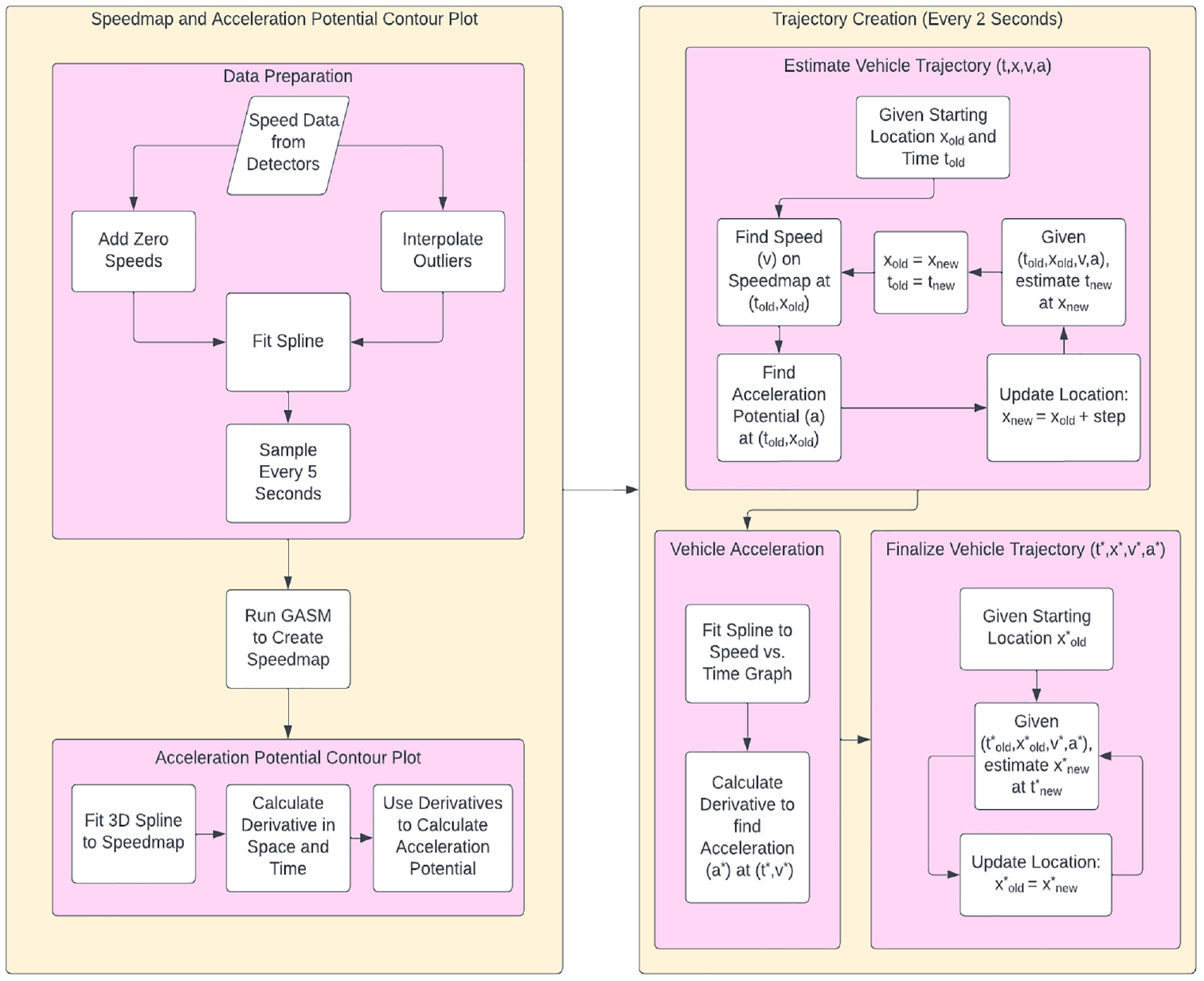
Flowchart depicting the process of developing hypothetical vehicle trajectories.

Based on the speedmap, vehicle trajectories were constructed using kinematics (discussed in the subsection on finding hypothetical vehicle trajectories). However, to increase the accuracy, the acceleration potential (i.e., the potential of the traffic stream to alter its speed) was used as an estimate of vehicle acceleration as described in the subsection finding acceleration potential. Once a trajectory was created, the speed versus time graph could be smoothed and the real acceleration found. However, a new trajectory needed to be created utilizing the smoothed speed and the acceleration calculated. This step aligned the vehicle location, speed, and acceleration at each point in time.

Finally, once each trajectory was created, and the speed and acceleration of every vehicle were known, the movements of the vehicles could be analyzed. Several metrics for analyzing vehicle trajectories can be developed, such as their maximum acceleration, and the average acceleration between their maximum and minimum speeds. Other metrics could include an evaluation of the environmental impacts by examining the speed and acceleration of each trajectory, or examinations of changes in travel times and the extent of congestion throughout the day.

Data Preparation

The methodology presented here is scalable, and can be applied to any road section. However, for the purposes of illustration, this study utilized data from a 2,665-ft segment of roadway on the I-94 westbound in Minneapolis, MN. Detector 1 was a Minnesota Department of Transportation detector, reporting average speeds every 30 s (x = 0 ft). Downstream at x = 1,250 ft, Detector 2 was a Houston Radar SpeedLane detector, reporting individual vehicle speed measurements. Finally, Detectors 3 and 4 (x = 2,025 ft and x = 2,665 ft, respectively) were Wavetronix radar detectors also reporting individual vehicle speed measurements. A diagram of these detectors along with their locations and lane configuration is presented in Figure 2.

Figure 2.

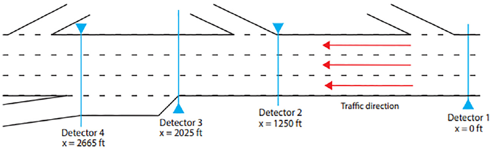
Study area: I-94 westbound near downtown Minneapolis, MN.

Figure 3 shows an example of raw data from these sensors. Some immediate differences were noted between these detectors. Figure 3a shows that the 30-s average speed data had far fewer outliers than the other data. However, these data did not show nearly the same resolution for the sharp speed changes observed that the other three data sources showed. This was unfortunate, since the goal was to detect these sharp changes in speed. Figure 3b depicts large bands of data, showing that Detector 2 had already processed some of the data before reporting it. In addition, there were no data points moving at speeds less than 6 mph. Finally, Figure 3, c and d , shows the data from the two Wavetronix sensors, which do not display as obvious a change to the data as the previous two. Furthermore, there were some data points below 5 mph (though not many). However, there were many outliers in these data. This was especially true in relation to the far lane of traffic from the detectors where there was more interference from the other two lanes.

Figure 3.

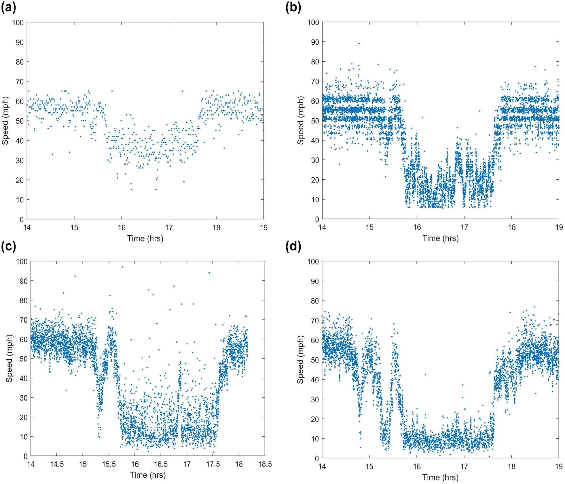
Vehicle speed measurements from each of the four detectors between 2:00 and 7:00 pm on October 19, 2020 (right-hand lane): (a) Detector 1: x = 0 ft; (b) Detector 2: x = 1,250 ft; (c) Detector 3: x = 2,025 ft; and (d) Detector 4: x = 2,665 ft.

In addition to the large number of outliers, another problem with this dataset was that it was not possible to have a speed of zero. This was because Doppler radar sensors cannot detect stationary vehicles, only slow-moving ones. Furthermore, it is rare for vehicles to stop exactly in front of a detector. Instead, they are usually detected when they are slowing down before stopping or accelerating having already stopped. For this reason, vehicles are most often detected at speeds of 5 to 10 mph. Figure 4 shows data from a single day that contain both of these problems. The inset on the left shows a series of points less than 20 mph with one outlier greater than 40 mph. The headway between the two adjacent vehicles traveling at a speed difference greater than 30 mph is only 2.5 s. The right-hand inset shows a series of vehicles moving as slow as 5 mph. At around Time 17.2 there was a headway of 34.5 s. This very large gap suggests that vehicles stopped between these two points. Examination of the video at this location confirmed both problems.

Figure 4.

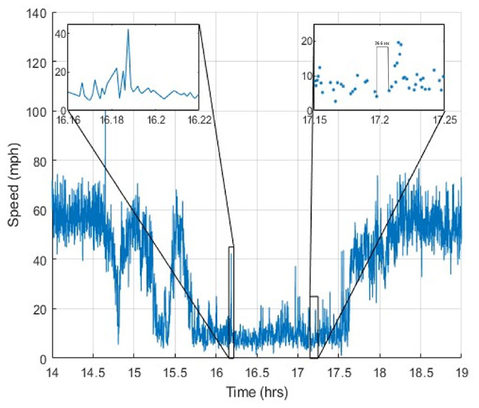
Individual vehicle speed measurements.

The first step in alleviating these problems is to correct for the outliers (often caused by sensors placing vehicles into incorrect lanes). This was accomplished through a moving mean of 20 data points and a threshold of 2.5 standard deviations from the mean. Outlier points were replaced with a linear interpolation between two neighboring points. However, the goal in the case study was to detect vehicles that were forced to decelerate quickly. Such vehicles are often moving slower than the vehicles around them. For this reason, only outliers with speeds above the mean were removed, and outliers with speeds below the mean were left in the data.

The next step was to introduce standing vehicle speeds into the data. Only the speed measurements were necessary to construct the speedmap, not flow or density. This meant that we were able to add data points at key locations to deepen the valleys in the speedmap without negatively influencing the results. This step was not necessary in the study undertaken by Treiber et al. because the GASM was originally designed using 30-s averaged speed data, and stops lasting over 30 s are rare ( 49 ). To add instances of zero speed to the individual vehicle speed data, we needed to make some assumptions about driver behavior. The first assumption was that vehicles traveling at speeds below 15 mph when crossing the detector could potentially be slowing to a stop or accelerating from a stop. Moreover, vehicles traveling at such slow speeds tend to travel in closely packed groups with small space headways. Moreover, vehicles traveling at such slow speeds tend to travel in closely packed groups with small space headways and mostly uniform time headways. If large gaps do occur, drivers tend use them to accelerate to higher speeds. For this reason, large time headways (i.e., greater than 5 s) at low speeds may indicate that vehicles have stopped between detections. We inserted a speed of zero between two vehicles if they were both traveling at less than 15 mph and the time headway between them was greater than 5 s. As these parameters were determined empirically, they were verified with video to confirm that vehicles were indeed involved in a queue.

Finally, a time series was created by using a spline fitted on the raw data ( 51 ). This spline was sampled every 5 s to estimate the speed of the traffic stream, which also reduced some of the most extreme perturbations in the data. This was a slightly higher resolution than the vehicle headways, so some data were lost. However, there was a trade-off between resolution and computational efficiency.

For the purposes of this study, all data were examined on a lane-by-lane basis. Though splitting the data by lane is not strictly necessary for any implementation, most roadways exhibit different patterns of congestion in different lanes. For this reason, averaging speeds across multiple lanes could lead to poor estimates of individual vehicle speeds and drastically affect the trajectory estimation process. For details on the different congestion propagation mechanisms at this location see the study by Robbennolt and Hourdos ( 52 ).

Speedmap Creation

Based on sparse data (in this example data from four point detectors), the speed of vehicles can be interpolated in time and space to approximate average traffic stream speeds. This was accomplished using the GASM discussed in Treiber and Helbing ( 50 ) and Treiber et al. ( 49 ). The input data were speed $(v_{ij})$ , at the locations of each detector $(x_{i})$ , and times when speed was known $(t_{j})$ . Although speed data from point detectors were used in this study, the GASM can utilize other sources of data such as trajectories from connected or probe vehicles to refine speedmap estimations.

The goal was to find the traffic speed, $V (x, t)$ , at all locations along the corridor, $x \in [x_{\min}, x_{\max}]$ , at all times, $t \in [t_{\min}, t_{\max}]$ . To do this, two filters, $Z_{cong} (x, t)$ and $Z_{free} (x, t)$ , were created, which corresponded to the expected propagation of speeds in congested and free flowing traffic. Equations 3 and 4 define these two filters. The filters were combined using a weight function to find the final velocity at every location.

V (x, t) = w (x, t) Z_{cong} (x, t) + [1 - w (x, t)] Z_{free} (x, t)

(1)

w (x, t) = \frac{1}{2} [1 + \tanh (\frac{V_{thr} - min [Z_{cong} (x, t), Z_{free} (x, t)]}{δ V})]

(2)

Z_{cong} (x, t) = \frac{\sum_{i} \sum_{j} ϕ (x_{i} - x, t_{j} - t + \frac{(x - x_{i})}{c_{cong}}) v_{ij}}{\sum_{i} \sum_{j} ϕ (x_{i} - x, t_{j} - t + \frac{(x - x_{i})}{c_{cong}})}

(3)

Z_{free} (x, t) = \frac{\sum_{i} \sum_{j} ϕ (x_{i} - x, t_{j} - t + \frac{(x - x_{i})}{c_{free}}) v_{ij}}{\sum_{i} \sum_{j} ϕ (x_{i} - x, t_{j} - t + \frac{(x - x_{i})}{c_{free}})}

(4)

ϕ (x, t) = \exp [- (\frac{x}{σ} + \frac{t}{τ})]

(5)

where

$v_{ij}$ = speed data from the sensors;

$x_{i}$ = locations in space of the sensors;

$t_{j}$ = times of data points collected at the sensors;

$V (x, t)$ = interpolated speed at every point in space and time;

$w (x, t)$ = weight function between the free flow and congested speed;

$Z_{free} (x, t)$ = filtered speed for free flow traffic;

$Z_{cong} (x, t)$ = filtered speed for congested traffic;

$V_{thr}$ = transition speed from free flow to congested flow;

$δ V$ = width of the transition region between congested flow and free flow;

$ϕ (x, t)$ = smoothing kernel of anisotropic filter;

$c_{cong}$ = congested wave speed;

$c_{free}$ = free flow wave speed;

$σ$ = range of spatial smoothing; and

$τ$ = range of temporal smoothing.

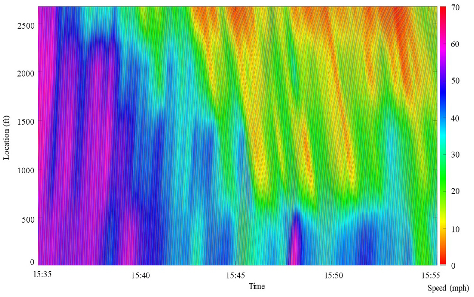
The values of $c_{cong}$ and $c_{free}$ were set based on known traffic flow patterns. In free flow traffic, perturbations travel downstream based on the movements of individual vehicles. Thus, $c_{free}$ was set close to the speed of vehicles in free flow. In congested traffic, shockwaves travel backward, against the flow of traffic. In this case, $c_{cong}$ was set to a negative value that was approximately the speed of those shockwaves.

This method is more effective than simple spatial interpolation in identifying what is happening between detectors, because it takes into account the estimated paths of any disturbances. The spatiotemporal interpolation effects can be seen in Figure 5: the lines illustrate the actual data along where each detector collects it. As can be seen from the figure, there were differences between the real data and the smoothed version at these locations because this method removed some of the more extreme variations in the detector data.

Figure 5.

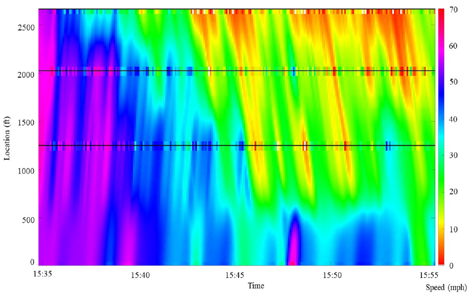
Spatiotemporal smoothing with real data plotted along detectors on October 19, 2021 (20-min window at the start of congestion).

Calibrating the GASM Model

The GASM model relied on six parameters: congested wave speed $(c_{cong})$ , free flow speed $(c_{free})$ , two parameters for transition speed ( $δ V$ and $V_{thr}$ ), and two smoothing parameters in space $(σ)$ and time $(τ)$ . These parameters needed to be calibrated for each new section of roadway since they corresponded to assumed parameters on the fundamental diagram. First, the values of $σ$ and $τ$ were calibrated to remove discontinuities in the speedmap. Then, a root mean square error (RMSE) minimization process on estimated traffic speeds was used to calibrate the other four parameters.

The two smoothing parameters in space $(σ)$ and time $(τ)$ were calibrated first on the speedmaps. Treiber et al. used the values of $τ = \frac{Δ t}{2}$ and $σ = \frac{Δ x}{2}$ , where $Δ x$ represents the spacing between detectors and $Δ t$ is the time between speed measurements ( 49 ). However, the distances between the detectors and the time between data points were much higher in their study. When lower values were used, irregularities were created. To avoid this phenomenon, each value was set to an arbitrarily small value and increased incrementally until the discontinuities were removed. This method determined the smallest sigma and tau values (i.e., the least smoothing) while still interpolating to reasonable values during the GASM process. The final values used in this study were $σ = 264$ ft and $τ = 6$ s. As in Treiber et al.’s study, the optimal $σ$ value was slightly less than half the distance between the detectors. However, a comparatively larger value of $τ$ was found to be optimal ( 49 ).

To perform the RMSE minimization, the speeds were estimated at Detector 3 (i.e., the middle of the three individual speed detectors) using the GASM. The objective of this process was to minimize the RMSE of vehicle speeds at this detector. The calibration program ran using data from nine separate shockwaves across seven different days. Of those cases, six came from the right-hand lane and three from the middle lane. Portions of the day with transitions between congested and free flow traffic were chosen for calibration since this transition is when conditions are typically more dangerous for drivers. These shockwaves were identified based on observations of video data. For optimization, a pattern search algorithm was used to calculate the objective at a mesh of points. The mesh was expanded and contracted around the lowest known objective until an optimal solution was found ( 53 ). For the calibration process only (and not subsequent to actually creating the final speedmaps), the data were smoothed to reduce noise and speed up the process. First, a 1-s spline was fit to the raw data and sampled every 1 s. To clean up this noise, a moving average with a window of 15 s and step size of 1 s was applied to the evenly spaced 1-s data. These data were then sampled only every 15 s.

In minimizing the RMSE of traffic speeds, several patterns emerged. The values of the free flow speed, $c_{free}$ , remained consistently at 35 mph. This value was lower than expected, but was understandable since vehicles tend to slow down as density increases and many were traveling at 35 to 40 mph even before any shockwaves occurred. This value was used as the forward propagation speed of perturbations, thus a value of 35 mph at peak density made sense. The calibrated congested wave speed, $c_{cong}$ , was between −11 and −18 mph. This is in the range we would generally expect to see for freeway traffic. Based on this information we set $c_{free} = 35$ mph and $c_{cong}$ = −17 mph, the most commonly occurring values.

The relationship between the transition speed, $V_{thr}$ , the width of the transition region, $δ V$ , and the weight function, $w (x, t)$ , is described in Equation 2. Figure 6 depicts how the weight changed with speed and various values of $V_{thr}$ and $δ V$ . $V_{thr}$ represents a translation of the weight between the two smoothing kernels, and $δ V$ relates to the slope of that transition. Taking this information into account, the width of the transition region had to be less than the speed difference between $c_{free}$ and $c_{cong}$ : $δ V < c_{free} + | c_{cong} |$ . Similarly, the transition speed itself had to fall between these two values: $c_{cong} < V_{thr} < c_{free}$ . Based on the calibrated results, it appeared that the choice of these parameters did not have a large effect on the RMSE. This was consistent with the findings of Treiber et al. ( 49 ). The calibrated values used for the final speedmaps were $V_{thr}$ = 30 mph and $δ V$ = 7 mph.

Figure 6.

Changes to the weight, $w (x, t)$ , with different values of transition speed, $V_{thr}$ , and transition region, $δ V$ .

Finding Acceleration Potential

Once the speedmap has been created, it can be further refined and a potential surface can be created. This is done by fitting a three-dimensional spline surface to the data. The data points can then be interpolated to get higher resolution traffic speed data. This is helpful in creating smoother trajectories.

In addition to interpolating the velocities to additional points, the spline surface provides a set of equations that define the data. The derivatives can be found in time and space, denoting a change in speed. The derivative of the speed with respect to time is the change in speed in time at a single point along the highway. Similarly the derivative with respect to space is the change in speed along the length of the highway at a constant time. Denote these two potentials as $P_{x}$ and $P_{t}$ , respectively, and define them as

P_{x} (x, t) = \frac{\partial V (x, t)}{\partial x}

(6)

P_{t} (x, t) = \frac{\partial V (x, t)}{\partial t}

(7)

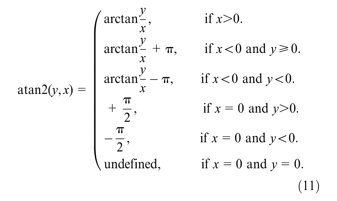
Based on these two partial derivatives of the speedmap, the gradient is defined as

\nabla V (x, t) = [P_{t} (x, t), P_{x} (x, t)]

(8)

The magnitude, $| | \nabla V (x, t) | |$ , and direction, $v$ , of this map can then be found,

| | \nabla V (x, t) | | = \sqrt{P_{t} {(x, t)}^{2} + P_{x} {(x, t)}^{2}}

(9)

θ = atan 2 [\frac{P_{t} (x, t)}{P_{x} (x, t)}]

(10)

where $atan 2$ is defined as

atan 2 (y, x) = (\begin{matrix} \arctan \frac{y}{x}, if x > 0 . \\ \arctan \frac{y}{x} + π, if x < 0 and y \geq 0 . \\ \arctan \frac{y}{x} - π, if x < 0 and y < 0 . \\ + \frac{π}{2}, if x = 0 and y > 0 . \\ - \frac{π}{2}, if x = 0 and y < 0 . \\ undefined, if x = 0 and y = 0 . \end{matrix}

(11)

The acceleration of a vehicle $(a)$ is $\frac{\partial V}{\partial t}$ . However, this derivative with respect to time needs to be taken along the trajectory of the vehicle moving in both space and time. This value cannot be calculated exactly since the trajectory of the vehicle is not known. Instead, the signed magnitude of the gradient is an approximation, which we termed acceleration potential,

a \approx | | \nabla V (x, t) | | \times \cos θ

(12)

Figure 7 shows a contour plot of the acceleration potential at every point in space and time along the roadway. Near the bottom of the figure, the acceleration potential was often close to zero. This was a result of the smoother data from the 30-s detector. However, there were some promising trends in the crisscrossing slopes of the free flow and congested wave speed around the other detectors. At higher speeds (uncongested) the trajectories of vehicles would follow these lines of acceleration, either not changing speed often or accelerating smoothly. At lower speeds (i.e., congested), the vehicles would instead frequently change speed and more sharply as they crossed these lines of acceleration propagating backward.

Figure 7.

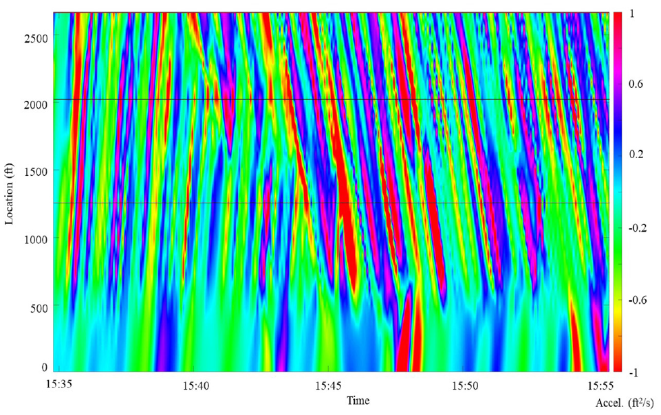
Contour plot of acceleration potential on October 19, 2021 (20-min window at the start of congestion).

This approximated acceleration can be used along with the velocities of the traffic to create each hypothetical trajectory as described in the following section.

Finding Hypothetical Vehicle Trajectories

The known speeds and approximated accelerations were used to find hypothetical vehicle trajectories. In this instance, these trajectories were not matched with the individual measurements at each of the detectors. Instead, we created a hypothetical trajectory every 2 s that represented the path a vehicle would have followed if it had actually been there. This initial time headway was chosen based on the case study presented below in which a decision was made by the algorithm every 2 s. For other applications a different headway between hypothetical vehicles could be more helpful, and could be used without any other changes to the methodology. Creating vehicles at this constant interval provided realistic velocity, acceleration, and positions for individual vehicles, but did not include anything meaningful about time and space headways between any two vehicles. For this reason, only measures of vehicle movements were applicable to these trajectories individually, not flow or density over several adjacent trajectories.

We created a hypothetical vehicle at the midpoint of the study area every 2 s and set its velocity and acceleration to that calculated on the speedmaps. The vehicle was then moved an arbitrarily small distance, $Δ x$ , along the corridor and its speed, acceleration, and travel time updated. Speed and acceleration will always be given by the speedmap as a function of location and time— $v (x, t)$ and $a (x, t)$ , respectively—and the time can be updated based on kinematics. This is accomplished by using the known speed and acceleration at the initial location to estimate the final velocity. That velocity can then be used to calculate the time the vehicle will arrive at the next location,

v_{f} = \sqrt{2 \times a \times Δ x + v_{i}^{2}}

(13)

t_{f} = t_{i} + \frac{2 \times Δ x}{(v_{f} + v_{i})}

(14)

where

$Δ x$ = difference in space between starting location, $x_{i}$ , and ending location, $x_{f}$ ;

$v_{i}$ = known velocity at location $x_{i}$ ;

$v_{f}$ = estimated velocity at location $x_{j}$ ;

$a$ = constant acceleration between locations $x_{i}$ and $x_{f}$ ;

$t_{i}$ = time at location $x_{i}$ ; and

$t_{f}$ = time at location $x_{j}$ .

This procedure was followed until each vehicle reached the end of the study area. Figure 8 shows a time–space diagram overlaid on the speedmap for a small section of the day.

Figure 8.

Time–space diagram overlaid on the speedmap on October 19, 2021 (20-min window at the start of congestion).

Calculating Vehicle Acceleration

Using the procedure outlined in the previous section, three quantities were known for each point along each trajectory: vehicle location at each time, speed, and acceleration potential. This information was used to calculate the actual acceleration of each vehicle at every point along the roadway instead of the acceleration potential.

Typically, trajectories are recorded as points in time and space. These can be differentiated with respect to time to find the velocity, and differentiated again to find the acceleration. However, speed was known, and this quantity had less introduced error than the calculated points of the trajectory since errors in vehicle position accumulated along the path of the vehicle. For this reason, these trajectories were analyzed as known speeds versus time points.

The trajectories derived from the speedmaps appeared to be very smooth in space. However, there were discontinuities in the speed because it could only be sampled at the same resolution as the speedmap. For this reason, a smoothing spline was fit to minimize the following objective:

p \sum_{i} (y_{i} - s (x_{i}))^{2} + (1 - p) \int {(\frac{d^{2} s}{d x^{2}})}^{2} dx

(15)

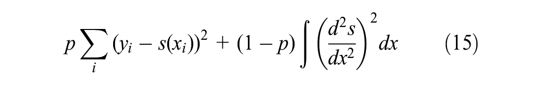
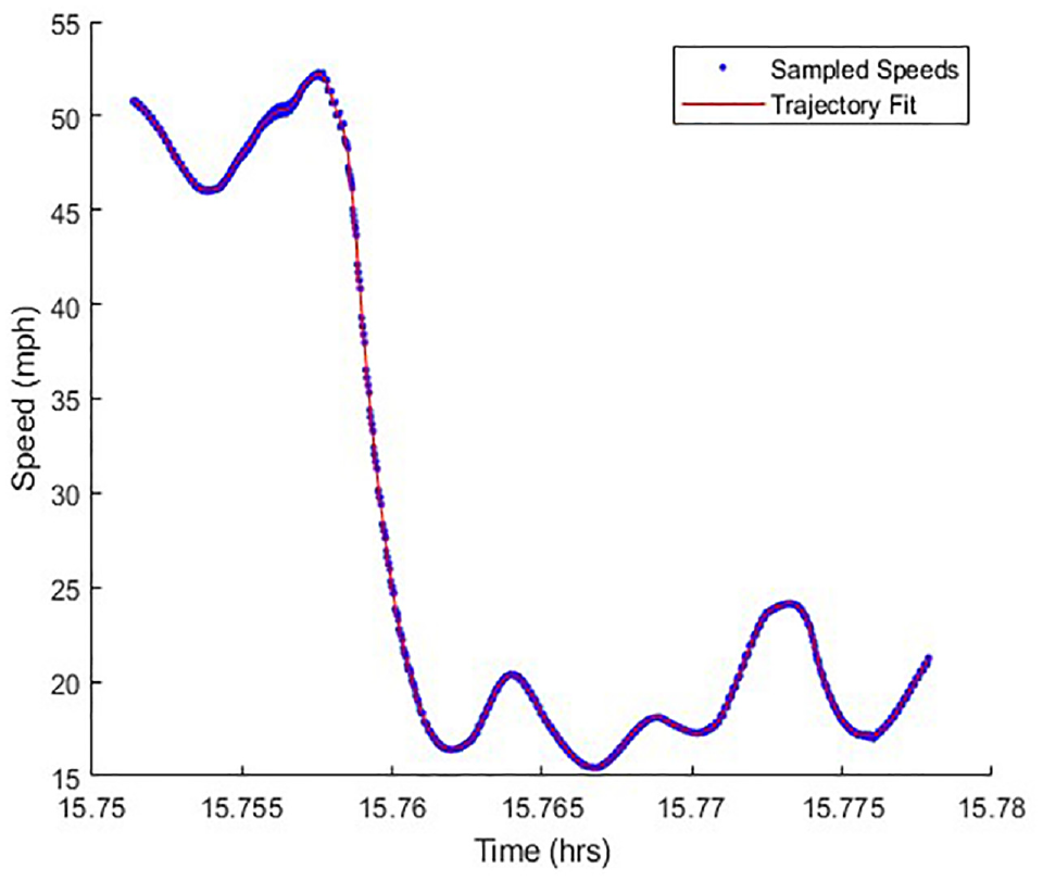
The parameter, p, was fit visually to ensure the fitted function followed the data as closely as possible without oscillating through each point. $p$ was set to 0.9185. This parameter needed to be high enough that it did not introduce curves into the straightest trajectories, but low enough that it followed the shape of all trajectories well. An example of the fitted curve is given in Figure 9.

Figure 9.

Speed versus location for a hypothetical trajectory-smoothing spline fit to the data.

The spline was fit to the speed versus time graph of the vehicle trajectory. The equations of this spline allowed for easy calculation of the instantaneous acceleration $(a)$ at every point by taking the derivative of the velocity $(v)$ with respect to time $(t)$ ,

a = \frac{dv}{dt}

(16)

Finally, with these new acceleration and speed values, the trajectory could be recalculated. This time, the sampled time points from the last iteration were left constant, and a new location was calculated. The change in the trajectory was very minimal, but this was an important step to keep all of the points aligned.

Sensitivity to Number of Detectors

It was important to understand the potential impacts of removing one of the detectors, as this could provide valuable information for future uses of this methodology, for example, facilitating decisions about how many detectors to install. In addition, throughout the study period of the case study detailed below, there were periods when the detectors were not functional. This analysis was helpful in determining whether there was still usable data from the days when that occurred.

This analysis used data from three separate weeks in late 2020 and in 2021. These 15 days were run with data from all four detectors, and then again with each of the four detectors excluded. This process revealed some valuable trends in the changes to the speedmaps, as well as in changes to the trajectories created. Of the days examined, March 16, 2020 had the largest differences when detectors were removed because the congestion came to an end between detectors in several locations. This caused problems when one detector was removed because the algorithm was not able to identify how far the congestion propagated between data points. Figure 10 contains a speedmap of the same day with each of the detectors removed. In addition, it depicts the absolute percent difference between the original speedmap and the modified version.

Figure 10.

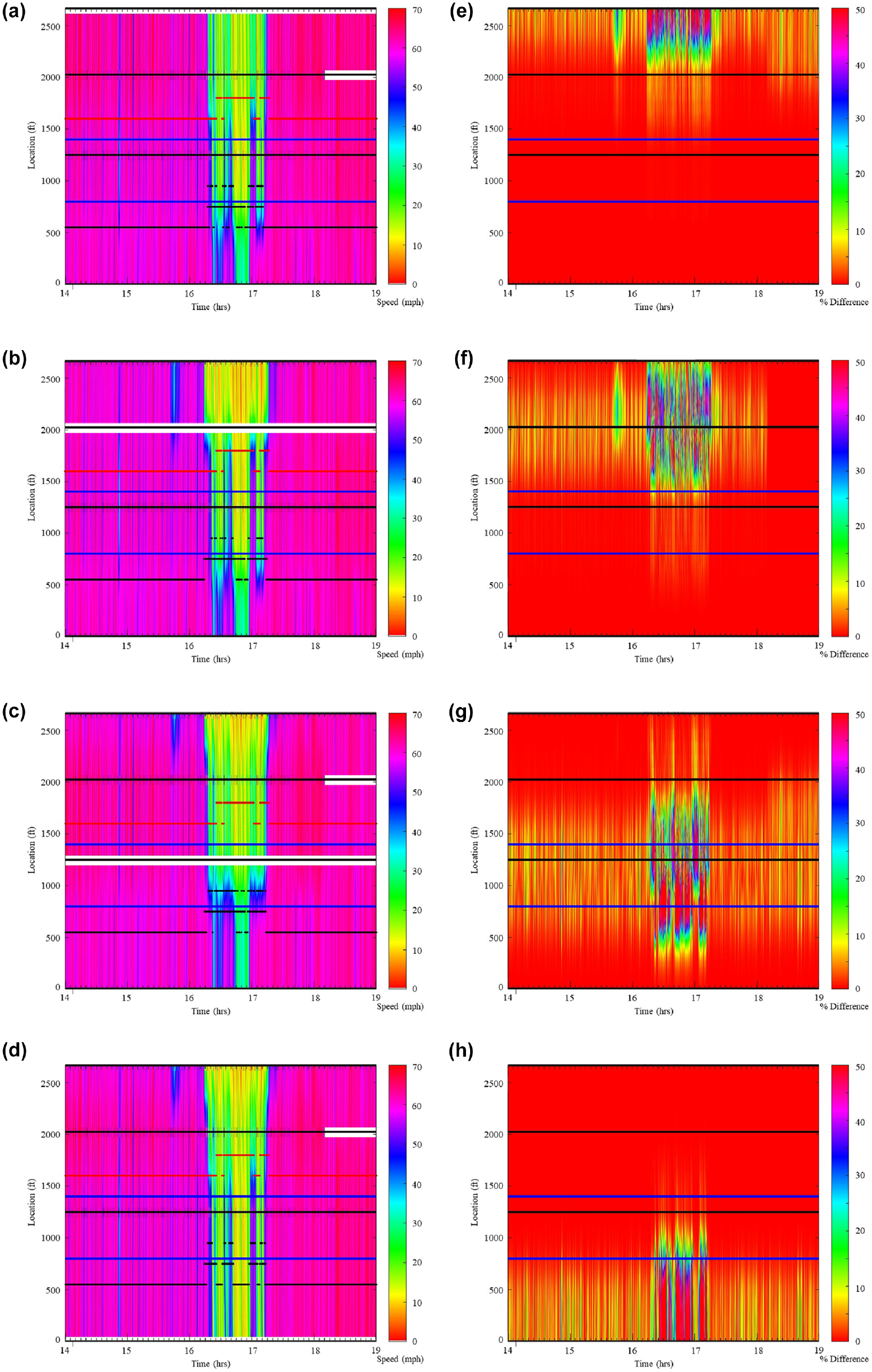
Speedmaps (a to d) when each detector is removed from the analysis. Percent difference when compared with the complete speedmap (e to h). Speedmaps: (a) no Detector 4, (b) no Detector 3, (c) no Detector 2, and (d) no Detector 1; acceleration maps: (e) no Detector 4, (f) no Detector 3, (g) no Detector 2, and (h) no Detector 1.

The biggest differences were observed where there was most congestion. One reason for this was that these numbers were smaller, so the percent differences increased at a faster rate. However, the speeds in the congested region were also more difficult to predict since the shockwaves were more pronounced and traveled backward. This caused large discrepancies to form when there were gaps between detectors. However, these errors persisted only between detectors. These deviations disappeared quickly once there were data from another detector because the GASM is a numerical heuristic that does not rely on the flow and density of traffic.

This methodology was utilized for the case study of a queue warning system (described in the subsection detailing implementation), in which the goal was to identify how information about dangerous conditions affected the traffic. We focused the generation of the trajectories into the high danger zone (resulting from geometrics), which in the rest of the document we refer to as the critical zone. The queue warning system was intended to warn drivers in this area experiencing dangerous conditions, so deceleration rates of hypothetical vehicles were calculated in the critical zone. For this reason, small discrepancies in deceleration rates were inconsequential outside that zone. The black dots on Figure 10, a to d , represents the trajectories with maximum deceleration (as described in the implementation subsection). It is clear from Figure 10 that the largest discrepancies were observed in the speedmaps in which the detectors were on either side of the critical zone, located at x = 0 ft and at x = 1,250 ft.

When comparing the number of vehicles in the high deceleration category between the 15 days studied, there was a significant difference depending on which detector was removed. If the detectors at x = 2,025 ft or x = 2,665 ft were removed, there was less than a 10% decrease in the number of high decelerations. On the other hand, if the detector at x = 0 ft was removed, there was a 41% decrease in the number of high decelerations and if the detector at x = 1,250 ft was removed, there was an increase of almost 300%. This suggests that (for the purposes of the case study) the detectors furthest upstream were much more important as they bound the critical zone.

This study took place on a 2,665-ft section of roadway with four detectors. Although we referred to this as a sparse dataset since we did not know what happened between the detectors, this methodology might also be an option where detector densities are lower. However, as shown, fewer detectors could lead to incorrect speed estimates. Since this was a short-term evaluation methodology, trailers with detectors could be placed for only a few weeks to increase detector density during the study period. In addition to the error in speed estimation, as the study corridor gets longer, vehicle position errors accumulate over long distances. A proposed numerical approach to reduce errors is to create trajectories starting from each detector to the midpoint between detectors and then stitching them together. This approach would reduce the accumulated errors in vehicle location over longer study areas.

Implementation

The method developed in this study could be widely applied to several different ATM systems, and used to evaluate them on different metrics. Some examples are described below, although this is not exhaustive.

Ramp metering is an ATM system that limits the number of vehicles entering a freeway. Researchers may be particularly interested in determining the travel time of vehicles, to determine whether this system is improving travel times or causing delays. In addition, examining the speeds of these trajectories in more detail can help pinpoint areas where delays are common.

When studying variable speed limits, researchers might be interested in compliance rates. A point detector at the sign might provide some information on compliance, but would not show how a speed limit might change driver behavior over a greater distance. In particular, hypothetical trajectory data could be helpful in examining the variation in speeds along the corridor to demonstrate whether the variable speed limit signs are helpful in smoothing traffic turbulence.

In this study, a queue warning system was evaluated to determine how accurate the system is in warning drivers approaching congestion. Since only the operation of the system itself was in question, evaluating conditions before implementation was not necessary. Instead, trajectories were examined for high deceleration rates that indicated unsafe conditions. The time these trajectories passed underneath the warning sign could be compared with the displayed message to evaluate the efficiency of the system.

This queue warning system operated on I-94 in Minneapolis, MN (the same roadway section used in previous examples). A changeable message sign was located at x = 0 ft. The goal of this system was to warn drivers as they approached the end of queues. This was the second implementation of the MN-QWARN system described in the research by Hourdos et al. ( 16 ). The deceleration rate of hypothetical vehicle trajectories was used as a surrogate safety measure to determine whether any dangerous behaviors were occurring. The queue warning system was implemented to warn drivers in the critical zone, located between x = 800 ft and x = 1,400 ft where visibility was lowest. This assumption implies that if drivers are before or after this region, visibility is good enough that even inattentive drivers will detect approaching shockwaves.

In the process of rating the trajectories, we made several assumptions. First, a speed of less than 20 mph on the speedmap represented significant traffic turbulence. Second, a maximum deceleration greater than 3 ft/s² was considered dangerous. Moreover, the average deceleration between the minimum and maximum speed of the vehicle had to be greater than 1.3 ft/s² for a trajectory to be considered dangerous. These values were calibrated using observations from video of the roadway and data from an independent radar. The average deceleration was found by finding the local maximum and minimum speeds on either side of the maximum deceleration. Then, the average acceleration, $\bar{a}$ , was

\bar{a} = \frac{v_{\max} - v_{\min}}{t_{\max} - t_{\min}}

(17)

where

$\bar{a}$ = average acceleration of the vehicle,

$v_{\max}$ = previous local maximum speed of the vehicle,

$v_{\min}$ = next local minimum speed of the vehicle,

$t_{\max}$ = time of previous local maximum speed of the vehicle, and

$t_{\min}$ = time of next local minimum speed of the vehicle.

In addition to having high deceleration rates, we required that vehicles entered the road segment at speeds higher than 30 mph and slowed down in response to the congestion to less than 20 mph. This ensured that vehicles were moving quickly when they had to apply their brakes, which put them at higher risk. It also ensured that they came to a stop at the end of a queue. If all these criteria were met, the trajectory was considered dangerous, and the driver should have been warned.

The rated trajectories could be used as a ground truth and compared with the function of the alarm. The detection rate was defined as the number of times the sign displayed a warning when a dangerous deceleration occurred, divided by the total number of high deceleration trajectories. Using data from September 1 to April 22, 2022 the right-hand lane had a detection rate of 21.2% and the left-hand lane had a detection rate of 60.6%. We also noted that there were fewer than 50 crashes during this time, many unrelated to congestion (e.g., drunk driving, lane-changing sideswipe under free flow, system was nonoperational). With so few data points, statistical conclusions were impossible to draw. At the same time, there were over 60,000 dangerous trajectories, making realistic conclusions possible even in the limited time horizon of this evaluation.

We can also dig deeper into these statistics by examining the detection rate of the first event of the day. On the very first event of the day, the detection rate was only 17.6% for the right-hand lane and the alarm was raised late 59.2% of the time. For the left-hand lane the detection rate was 24.3% and the alarm was raised late 67.4% of the time. These statistics are helpful in demonstrating that the queue warning algorithm was not sensitive enough to dangerous conditions, particularly at the onset of congestion. For more details on the second implementation of the described queue warning system, refer to the study by Robbennolt and Hourdos ( 52 ).

Conclusion

This paper presents a methodology that can be used to estimate the trajectories of hypothetical vehicles based on sparse detector data. Owing to the larger number of high deceleration events than there were crashes, the methodology presented was faster than a traffic safety study, which can take 3 to 5 years before and after implementation of an ATM system. In addition, the high-resolution trajectories were created from real roadway data (an improvement over microsimulation studies). Trajectory estimation relied on the GASM developed in the study by Treiber et al. to estimate the speed at every point in time and space along the roadway ( 49 ). Vehicle trajectories could be created from this speedmap, describing vehicle location in space and time as well as providing speed and acceleration data at each point. As discussed, these trajectories could be used to evaluate changes to traffic flow when new ATM systems or TSMO strategies are introduced. In this paper, the methodology was demonstrated using vehicle deceleration rates to evaluate the detection rate of a queue warning algorithm. Other implementations might evaluate travel time, the extent of congestion, and environmental impacts utilizing information from the trajectories.

Future improvements to this methodology should focus on the speedmaps, since trajectories are built based on the speedmaps alone. However, these speedmaps provide no information about the flow or density of the traffic. This means that the trajectories are created at a constant 2 s apart and headways therefore cannot be used meaningfully. Incorporating flow and density would improve the congestion propagation on the speedmaps and allow the trajectories to be created at more realistic intervals. Another area for future work would be to compare the hypothetical trajectories with real trajectories from the roadway (collected using probe vehicles or radar detectors). This research demonstrated that it is possible to create these trajectories and extract meaningful information. However, a closer comparison to real trajectories could lead to more improvements, as deviations from the estimations could be studied in detail. Along similar lines, this methodology should be tested against simulation data to examine the relative accuracy of the trajectory estimation methodology as a whole.

Footnotes

Author Contributions

The authors confirm contribution to the paper as follows: study conception and design: J. Robbennolt, J. Hourdos; data collection: J. Hourdos; analysis and interpretation of results: J. Robbennolt, J. Hourdos; draft manuscript preparation: J. Robbennolt, J. Hourdos. All authors reviewed the results and approved the final version of the manuscript.

Declaration of Conflicting Interests

The authors declared no potential conflicts of interest with respect to the research, authorship, and/or publication of this article.

Funding

The authors disclosed receipt of the following financial support for the research, authorship, and/or publication of this article: This project was fully funded by the Minnesota Department of Transportation and utilized instrumentation of the Minnesota Traffic Observatory that was funded earlier as part of the Roadway Safety Institute Regional University Transportation Center (c) 1003325 (wo) 84.

ORCID iDs

Jake Robbennolt

John Hourdos

References

Xiong

Yang

X. T.

Zhang

Lee

Zhou

Raqib

An Integrated Modeling Framework for Active Traffic Management and Its Applications in the Washington, DC Area. Journal of Intelligent Transportation Systems, Vol. 25, No. 6, 2021, pp. 609–625. https://doi.org/10.1080/15472450.2021.1878891.

Iordanidou

G.-R.

Papamichail

Roncoli

Papageorgiou

Feedback-Based Integrated Motorway Traffic Flow Control with Delay Balancing. IEEE Transactions on Intelligent Transportation Systems, Vol. 18, No. 9, 2017, pp. 2319–2329. https://doi.org/10.1109/TITS.2016.2636302.

Yang

Lin

Zou

Optimal Variable Speed Limit Control for Real-Time Freeway Congestions. Procedia-Social and Behavioral Sciences, Vol. 96, 2013, pp. 2362–2372. https://doi.org/10.1016/j.sbspro.2013.08.265; https://linkinghub.elsevier.com/retrieve/pii/S1877042813023914.

Zhang

Levinson

Balancing Efficiency and Equity of Ramp Meters. Journal of Transportation Engineering, Vol. 131, No. 6, 2005, pp. 477–481. https://doi.org/10.1061/(ASCE)0733-947X(2005)131:6(477); http://ascelibrary.org/doi/10.1061/%28ASCE%290733-947X%282005%29131%3A6%28477%29.

National Research Council. Highway Safety Manual. 1st ed. American Association of State Highway and Transportation Officials, Washington, D.C., 2010.

Piotrowicz

Robinson

Ramp Metering Status in North America, 1995 Update. Technical Report. DOT-T-95-17. Federal Highway Administration, 1995. https://rosap.ntl.bts.gov/view/dot/2703.

Cleavenger

D. K.

Upchurch

Effect of Freeway Ramp Metering on Accidents: The Arizona Experience. ITE Journal, Vol. 69, No. 8. https://trid.trb.org/view/506749.

Chambers

A. L.

Benefits of Advanced Traffic Management Solutions: Before and After Crash Analysis for Deployment of a Variable Advisory Speed Limit System. PhD thesis. California Polytechnic State University, San Luis Obispo, 2016. https://digitalcommons.calpoly.edu/theses/1653.

Dutta

Fontaine

Boetang

Campbell

Evaluation of the Impact of the I-66 Active Traffic Management System: Phase II. Technical Report. VTRC 19-R7. Virginia Transportation Research Council, Charlottesville, 2018.

10.

Liu

Wang

Ramp Metering Influence on Freeway Operational Safety near On-Ramp Exits. International Journal of Transportation Science and Technology, Vol. 2, No. 2, 2013, pp. 87–94. https://doi.org/10.1260/2046-0430.2.2.87; https://www.sciencedirect.com/science/article/pii/S2046043016300788.

11.

Hourdos

Parikh

Dirks

Lehrke

Lukashin

Evaluation of the Smart Work Zone Speed Notification System. Technical Report. MN/RC 2019-21. Minnesota Department of Transportation, St. Paul, MN, 2019.

12.

Lin

Wang

Sadek

A. W.

A Novel Variable Selection Method Based on Frequent Pattern Tree for Real-Time Traffic Accident Risk Prediction. Transportation Research Part C: Emerging Technologies, Vol. 55, 2015, pp. 444–459. https://doi.org/10.1016/j.trc.2015.03.015; https://linkinghub.elsevier.com/retrieve/pii/S0968090X15000947.

13.

Hébert

Guédon

Glatard

Jaumard

High-Resolution Road Vehicle Collision Prediction for the City of Montreal. Proc., 2019 IEEE International Conference on Big Data (Big Data), Los Angeles, CA, IEEE, New York, 2019, pp. 1804–1813. https://doi.org/10.1109/BigData47090.2019.9006009.

14.

Abdel-Aty

Real-Time Crash Likelihood Prediction Using Temporal Attention–Based Deep Learning and Trajectory Fusion. Journal of Transportation Engineering, Part A: Systems, Vol. 148, No. 7, 2022, p. 04022043. https://doi.org/10.1061/JTEPBS.0000697. https://ascelibrary.org/doi/full/10.1061/JTEPBS.0000697.

15.

Pei

Wong

Sze

A Joint-Probability Approach to Crash Prediction Models. Accident Analysis & Prevention, Vol. 43, No. 3, 2011, pp. 1160–1166. https://doi.org/10.1016/j.aap.2010.12.026. https://linkinghub.elsevier.com/retrieve/pii/S0001457510004033.

16.

Hourdos

Duhn

Liu

Parikh

Evaluation of the Minnesota Queue Warning System, MN-QWARN. Number: TRBAM-21-04057. Presented at 100th Annual Meeting of the Transportation Research Board, Washington, D.C., 2021. https://trid.trb.org/view/1759599.

17.

Tarko

A. P.

Wang

Liu

Predicting Crash Likelihood and Severity on Freeways with Real-Time Loop Detector Data. Accident Analysis & Prevention, Vol. 57, 2013, pp. 30–39. https://doi.org/10.1016/j.aap.2013.03.035; https://www.sciencedirect.com/science/article/pii/S0001457513001334.

18.

Joshi

Surrogate Safety Assessment Model (SSAM): Software User Manual. Technical Report. FHWA-HRT-08-050. Federal Highway Administration, 2008. https://www.fhwa.dot.gov/publications/research/safety/08050/08050.pdf.

19.

Ariza

Validation of Road Safety Surrogate Measures as a Predictor of Crash Frequency Rates on a Large-Scale Microsimulation Network. PhD thesis. University of Toronto, Ontario, Canada, 2011.

20.

Ghanim

M. S.

Shaaban

A Case Study for Surrogate Safety Assessment Model in Predicting Real-Life Conflicts. Arabian Journal for Science and Engineering, Vol. 44, No. 5, 2019, pp. 4225–4231. https://doi.org/10.1007/s13369-018-3326-8; http://link.springer.com/10.1007/s13369-018-3326-8.

21.

Hourdakis

Michalopoulos

P. G.

Evaluation of Ramp Control Effectiveness in Two Twin Cities Freeways. Transportation Research Record: Journal of the Transportation Research Board, 2002. 1811: 21–29.

22.

Abdel-Aty

Haleem

Cunningham

Gayah

Application of Variable Speed Limits and Ramp Metering to Improve Safety and Efficiency of Freeways. Proc., 2nd International Symposium on Freeway and Tollway Operations, Honolulu, HI, 2009.

23.

Lee

Hellinga

Ozbay

Quantifying Effects of Ramp Metering on Freeway Safety. Accident Analysis & Prevention, Vol. 38, No. 2, 2006, pp. 279–288. https://doi.org/10.1016/j.aap.2005.09.011; https://www.sciencedirect.com/science/article/pii/S000145750500151X.

24.

Karim

H. K.

Exploratory Analysis of Ramp Metering on Efficiency, and Safety of Freeways Using Microsimulation. PhD dissertation. University of Kansas, Lawrence, 2015. https://kuscholarworks.ku.edu/handle/1808/20979.

25.

Abdel-Aty

Dilmore

Dhindsa

Evaluation of Variable Speed Limits for Real-Time Freeway Safety Improvement. Accident Analysis & Prevention, Vol. 38, No. 2, 2006, pp. 335–345. https://doi.org/10.1016/j.aap.2005.10.010; https://www.sciencedirect.com/science/article/pii/S0001457505001764.

26.

Abdel-Aty

Gayah

Real-Time Crash Risk Reduction on Freeways Using Coordinated and Uncoordinated Ramp Metering Approaches. Journal of Transportation Engineering, Vol. 136, No. 5, 2010, pp. 410–423. https://doi.org/10.1061/(ASCE)TE.1943-5436.0000100; https://ascelibrary.org/doi/10.1061/%28ASCE%29TE.1943-5436.0000100.

27.

Nezamuddin

Jiang

Zhang

Waller

S. T.

Sun

Traffic Operations and Safety Benefits of Active Traffic Strategies on TxDOT Freeways. Technical Report. FHWA/TX-12/0-6576-1. Center for Transportation Research, The University of Texas at Austin, 2011. https://trid.trb.org/view/1144068.

28.

Nezamuddin

Jiang

Zhang

Waller

S. T.

Active Traffic Management Strategies: Implications for Freeway Operations and Traffic Safety. Presented at 90th Annual Meeting of the Transportation Research Board, Washington, D.C., 2011. https://trid.trb.org/view/1092841.

29.

Wang

Abdel-Aty

Lee

Implementation of Active Traffic Management Strategies for Safety on Congested Expressway Weaving Segments. Transportation Research Record: Journal of the Transportation Research Board, 2017. 2635: 28–35.

30.

Lee

S. M.

Shokri

A. A.

Al-Mansour

A. I.

Evaluation of the Applicability of the Ramp Metering to a Freeway Using Microsimulation: A Case Study in Riyadh, Saudi Arabia. Applied Sciences, Vol. 9, No. 20, 2019, p. 4406. https://doi.org/10.3390/app9204406; https://www.mdpi.com/2076-3417/9/20/4406.

31.

Wang

Abdel-Aty

Active Traffic Management Strategies for Expressways Based on Crash Risk Prediction of Moving Vehicle Groups. Accident Analysis & Prevention, Vol. 163, 2021, p. 106421. https://doi.org/10.1016/j.aap.2021.106421. https://www.sciencedirect.com/science/article/pii/S0001457521004528.

32.

Chen

Levin

Hourdos

Duhn

Generating Traffic Information from Connected Vehicle V2V Basic Safety Messages. Technical Report. MN 2021-08. Minnesota Department of Transportation, St. Paul, 2021.

33.

Stanitsas

Hourdos

Zitzow

Evaluation of the Effect of MnPASS Lane Design on Mobility and Safety. Technical Report. MN/RC 2014-23. Minnesota Department of Transportation, St. Paul, 2014. https://www.lrrb.org/pdf/201423.pdf.

34.

Mudgal

Hourdos

Impact of Variable Speed Limits on Freeway Rear-End Collisions. Presented at 96th Annual Meeting of the Transportation Research Board, Washington, D.C., 2017. https://trid.trb.org/view/1439052.

35.

Han

Meng

Zheng

Liu

An Urban Freeway Ramp Metering Control System Based on Trajectory Data. Presented at 98th Annual Meeting of the Transportation Research Board, Washington, D.C., 2019. https://trid.trb.org/view/1573413.

36.

Wang

Shen

Bezzina

Sayer

J. R.

Liu

H. X.

Feng

Data Infrastructure for Connected Vehicle Applications. Transportation Research Record: Journal of the Transportation Research Board, 2020. 2674: 85–96.

37.

Yao

Liu

Jiang

Tang

Ran

Trajectory Reconstruction for Mixed Traffic Flow with Regular, Connected, and Connected Automated Vehicles on Freeway. IET Intelligent Transport Systems, Vol. n/a, No. n/a, 2022. https://doi.org/10.1049/itr2.12294; https://onlinelibrary.wiley.com/doi/abs/10.1049/itr2.12294.

38.

Wang

Wei

Chen

Trajectory Reconstruction for Freeway Traffic Mixed with Human-Driven Vehicles and Connected and Automated Vehicles. Transportation Research Part C: Emerging Technologies, Vol. 111, 2020, pp. 135–155. https://doi.org/10.1016/j.trc.2019.12.002; https://www.sciencedirect.com/science/article/pii/S0968090X19307818.

39.

Haule

H. J.

Ali

M. S.

Alluri

Sando

Evaluating the Effect of Ramp Metering on Freeway Safety Using Real-Time Traffic Data. Accident Analysis & Prevention, Vol. 157, 2021, p. 106181. https://doi.org/10.1016/j.aap.2021.106181; https://www.sciencedirect.com/science/article/pii/S0001457521002128.

40.

Ahn

Bertini

R. L.

Auffray

Ross

J. H.

Eshel

Evaluating Benefits of Systemwide Adaptive Ramp-Metering Strategy in Portland, Oregon. Transportation Research Record: Journal of the Transportation Research Board, 2007. 2012: 47–56.

41.

Levinson

Zhang

Ramp Meters on Trial: Evidence from the Twin Cities Metering Holiday. Transportation Research Part A: Policy and Practice, Vol. 40, No. 10, 2006, pp. 810–828. https://doi.org/10.1016/j.tra.2004.12.004; https://linkinghub.elsevier.com/retrieve/pii/S0965856406000024.

42.

Zhang

Vehicle Trajectory Reconstruction on Urban Traffic Network Using Automatic License Plate Recognition Data. IEEE Access, Vol. 9, 2021, pp. 49110–49120. https://doi.org/10.1109/ACCESS.2021.3068964.

43.

Rose

Sarvi

Evaluation of Speed-Based Travel Time Estimation Models. Journal of Transportation Engineering, Vol. 132, No. 7, 2006, pp. 540–547. https://doi.org/10.1061/(ASCE)0733-947X(2006)132:7(540); http://ascelibrary.org/doi/10.1061/%28ASCE%290733-947X%282006%29132%3A7%28540%29.

44.

van Lint

J. W. C.

Van der Zijpp

N. J.

Improving a Travel-Time Estimation Algorithm by Using Dual Loop Detectors. Transportation Research Record: Journal of the Transportation Research Board, 2003. 1855: 41–48.

45.

Yang

Tian

An Exploratory Investigation of the Impact of Ramp Metering on Driver Acceleration Behavior. IATSS Research, Vol. 43, No. 4, 2019, pp. 277–285. https://doi.org/10.1016/j.iatssr.2019.03.002; https://www.sciencedirect.com/science/article/pii/S0386111218301407.

46.

Chakroborty

Kikuchi

Using Bus Travel Time Data to Estimate Travel Times on Urban Corridors. Transportation Research Record: Journal of the Transportation Research Board, 2004. 1870: 18–25.

47.

Wei

Wang

Chen

A Particle Filter-Based Approach for Vehicle Trajectory Reconstruction Using Sparse Probe Data. IEEE Transactions on Intelligent Transportation Systems, Vol. 22, No. 5, 2021, pp. 2878–2890. https://doi.org/10.1109/TITS.2020.2976671.

48.

Cortés

C. E.

Lavanya

J.-S.

Jayakrishnan

General-Purpose Methodology for Estimating Link Travel Time with Multiple-Point Detection of Traffic. Transportation Research Record: Journal of the Transportation Research Board, 2002. 1802: 181–189.

49.

Treiber

Kesting

Wilson

R. E.

Reconstructing the Traffic State by Fusion of Heterogeneous Data. Computer-Aided Civil and Infrastructure Engineering, Vol. 26, No. 6, 2009, pp. 408–419. https://doi.org/10.1111/j.1467-8667.2010.00698.x

50.

Treiber

Helbing

Reconstructing the Spatio-Temporal Traffic Dynamics from Stationary Detector Data. Cooper@tive Tr@nsport@tion Dyn@mics, Vol. 1, 2002, pp. 3.1–3.24.

51.

Fritsch

F. N.

Carlson

R. E.

Monotone Piecewise Cubic Interpolation. SIAM Journal on Numerical Analysis, Vol. 17, No. 2, 1980, pp. 238–246. https://doi.org/10.1137/0717021; https://epubs.siam.org/doi/10.1137/0717021.

52.

Robbennolt

Hourdos

Evaluation of the Second Implementation of the Minnesota Queue Warning System: MNQWARN. Presented at 100th Annual Meeting of the Transportation Research Board, Washington, D.C., 2023. https://trid.trb.org/view/1759599.

53.

Audet

Dennis

J. E.

Analysis of Generalized Pattern Searches. SIAM Journal on Optimization, Vol. 13, No. 3, 2002, pp. 889–903. https://doi.org/10.1137/S1052623400378742; https://epubs.siam.org/doi/10.1137/S1052623400378742.

Data-Driven Evaluation Methodology for Active Traffic Management Systems Utilizing Sparse Speed Data

Abstract

Keywords

Background

Methodology

Data Preparation

Speedmap Creation

Calibrating the GASM Model

Finding Acceleration Potential

Finding Hypothetical Vehicle Trajectories

Calculating Vehicle Acceleration

Sensitivity to Number of Detectors

Implementation

Conclusion

Footnotes

Author Contributions

Declaration of Conflicting Interests

Funding

ORCID iDs

References