Decision Tree Analysis for Developing Weigh-in-Motion Spectra in the Californian Pavement Management System (PaveM)

Abstract

Weigh-in-motion (WIM) devices record vehicle axle loads on highways. WIM data include axle loads, inter-axle spacings, vehicle classification, gross vehicle weights, vehicle length, and travel speed. Pavement design, management, and performance studies all require WIM data, directly as a spectrum or indirectly as standard axles. In 2016, 132 WIM devices were operating on California’s highway network, one of the densest and best-maintained clusters in the United States. The University of California Pavement Research Center (UCPRC) has been working with these data since 2002, and it completed the analysis of data collected from 1998 to 2003 in 2008. This research investigated similarities in axle load distributions at the WIM sites and grouped them to generate traffic inputs for pavement design. This paper is an extension of that work, including processing the 2004–2015 data from 80 WIM sites, identifying the axle load distribution for each site, updating the original groupings, and developing a new procedure to assign WIM spectra to other locations. For the past 11 years, axle loads and gross vehicle weight showed similar patterns, but average truck speeds decreased by 11%. A combination of clustering and cut-tree analysis was used to create a decision tree to classify the stations’ data into five WIM axle load spectra. The methodology has been used to compute traffic for the entire network used in the Caltrans pavement management system, PaveM. An application tool was also developed for generating truck traffic input files for the CalME and PavementME design tools.

The environment, traffic, and the interaction of the two cause pavements to deteriorate. Highway pavements sustain nearly all the traffic related to heavy trucks but nearly none from lighter vehicles. So, it is critical to understand the distribution of axle loads on any particular pavement for any pavement design, performance prediction, or management. As a result, considerable cost and effort is put into measuring vehicle loads by most road agencies. The primary tool for these measurements is the weigh-in-motion (WIM) station. WIM systems continuously measure and store loads and axle spacing data for each truck that passes through the WIM site ( 1 ). In 2016, 132 WIM devices were operating on the California state highway network, one of the densest and best-maintained clusters in the United States. However, these still only cover a fraction of the highway network, and a method is thus needed to predict the axle loads on the reminder of the network. The University of California Pavement Research Center (UCPRC) has been working with the California Department of Transportation (Caltrans) WIM data since 2002 and, in 2008, published an analysis of data collected from 1998 to 2003. This research investigated similarities in axle load distributions at the WIM sites, grouping them into averaged distributions, and presented a decision tree–based approach to generating traffic inputs for pavement design.

Mechanistic–Empirical (ME) Pavement Design Guide (MEPDG) procedures for both rigid and flexible pavement types have, since 2000, been evaluated for use in California by Caltrans and the UCPRC ( 1 ), including the development of a flexible pavement design procedure specifically for California known as CalME ( 2 ). These modern design methods use the full axle load spectrum to predict damage. An axle load spectrum is the load distribution of an axle group during a period ( 3 ). In addition, Caltrans has been developing and implementing a new pavement management system (PMS) since 2010, known as PaveM. This requires predicting future performance on all network segments, which in turn requires some prediction of the traffic loads on the entire network.

Background

WIM

WIM is a state-of-the-art system to collect, process, and store vehicular data from key locations on highways in California. Caltrans has been installing the WIM sites and collecting truck traffic data on the state highways in California since 1987. It maintains a detailed historical truck traffic information database for more than 120 highway sites across California. Currently, two categories of WIM systems are used in California: regular data collection and weigh site bypass. The former is used to collect traffic data on highways in California, while the latter is used in the PrePass™ operation to enable registered heavy vehicles to bypass open weigh sites after electronic verification legally. In the bypass WIM system, no data are stored except for the purpose of performance checks on the WIM. Therefore, all the data analyzed in this report came from the regular WIM data collection sites ( 4 ).

WIM systems consist of bending plate scales, which determine the wheel load estimates, and inductive loop detectors, which determine the vehicle’s presence, vehicle speed, and overall vehicle lengths. The bending plates are steel, typically 2–3 in. thick, 20–24 in. wide, and 6 ft across, secured in frames and anchored and epoxy bonded into the pavement. With the odd exception, Caltrans uses the “in-line” configuration, which consists of two bending plates installed side by side in each lane, one bending plate for each wheel path.

WIM systems record instantaneous dynamic axle loads and axle spaces, the number of axles, vehicle speed, overall vehicle length, lane and direction of travel, and the date and time a vehicle is passing over the sensors. WIM systems are calibrated with the intent, in part, that the system generates the best possible estimate of the static gross weights and the portions of those gross weights carried by each wheel for most of the vehicles passing through the WIM site. These accuracy of these systems primarily depends on the vehicle dynamics and the inherent variance of the technology used within the WIM system. A structurally sound and extremely smooth pavement is critical to a WIM system’s ability to generate accurate wheel load estimates ( 2 ).

Many researchers have analyzed WIM data with various approaches for truck traffic studies and traffic input generation for MEPDG software in many states, including California, Louisiana, North Carolina, and Virginia ( 2 , 5–8). Ishak et al. ( 6 ) grouped the portable WIM sites in Louisiana based on the degree of similarity between two distributions from a pair of sites, which was measured by the sum of squared difference between the two axle load distributions at the corresponding intervals and further analyzed axle load spectra by traffic truck classification groups. However, they were not able to capture seasonal and long-term variations because the 48-h data were collected at portable WIM sites. In North Carolina, Sayyday et al. ( 7 ) conducted hierarchical clustering analysis and post-clustering analysis for each axle load with four traffic parameters: truck volume, truck percentage, the ratio of class 5 to class 9 trucks, and the ratio of vehicle classes 4–7 to vehicle classes 8–13. Smith et al. ( 8 ) analyzed 15 WIM sites in Virginia to develop site-specific traffic data inputs for the MEPDG method. They compared the site-specific axle load spectra with the MEPDG defaults using the WIM-based and non-WIM-based parameters and showed the difference between them. Swan et al. ( 9 ) conducted a sensitivity analysis of the predicted pavement performances for the MEPDG software’s default traffic input parameters and the site-specific parameters in Ontario, Canada, and found a notable difference in axle load spectra.

The literature results above emphasize that axle load spectra should be developed with the site-specific traffic parameters by regions for accurate performance analysis in MEPDG methods instead of using the default ones.

Study Objectives

This study analyzed the axle load spectra and tuck traffic volumes with California’s latest WIM data set and developed a set of representative axle load spectra associated with the characteristic of highway segments ( 10 ). An application tool was then developed for generating the truck traffic inputs for ASSHTOWare PavementME Design and CalME for each pavement segment for highway networks in California and for performance models in the PMS, PaveM.

The objectives of this study were to:

1. Archive the binary files of available Caltrans WIM data, clean them. and convert them into a relational database to provide easy access and computation.

2. Group the WIM sites by the similarity of axle load spectra using statistical approaches.

3. Develop an application tool of a traffic calculator to generate traffic input files for pavement ME design tools.

4. Develop equivalent single axle load (ESAL) estimates for the entire state highway network for PaveM.

Overall Approach

The binary data files achieved in the Californian WIM sites from 2004 to 2015 were converted to readable formats with the Caltrans vehicle classification setting using the iAnalyzer^® tool developed by International Road Dynamics, Inc. ( 11 ). The sampled ASCII files were imported into the PostgreSQL database. The cluster analysis aggregated the 80 WIM sites into seven WIM groups by the similarity of each axle load spectra, and the cut-tree analysis produced a decision tree that categorized them into five WIM axle load spectra, using explanatory variables from the other databases available on the network (highway log and traffic information). The final five WIM axle load spectra were applied to PaveM highway segments to determine their axle load spectra for pavement management. An application tool for traffic calculation was developed to generate the traffic input files for AASHTOWare Pavement ME Design (MEPDG). The updated axle load spectra by using the latest decade of WIM data are used in the MEPDG, CalME, PaveM, and life cycle assessment (LCA) application tools. Figure 1 illustrates the study flow of the overall approach for updating WIM spectra and their applications.

Figure 1.

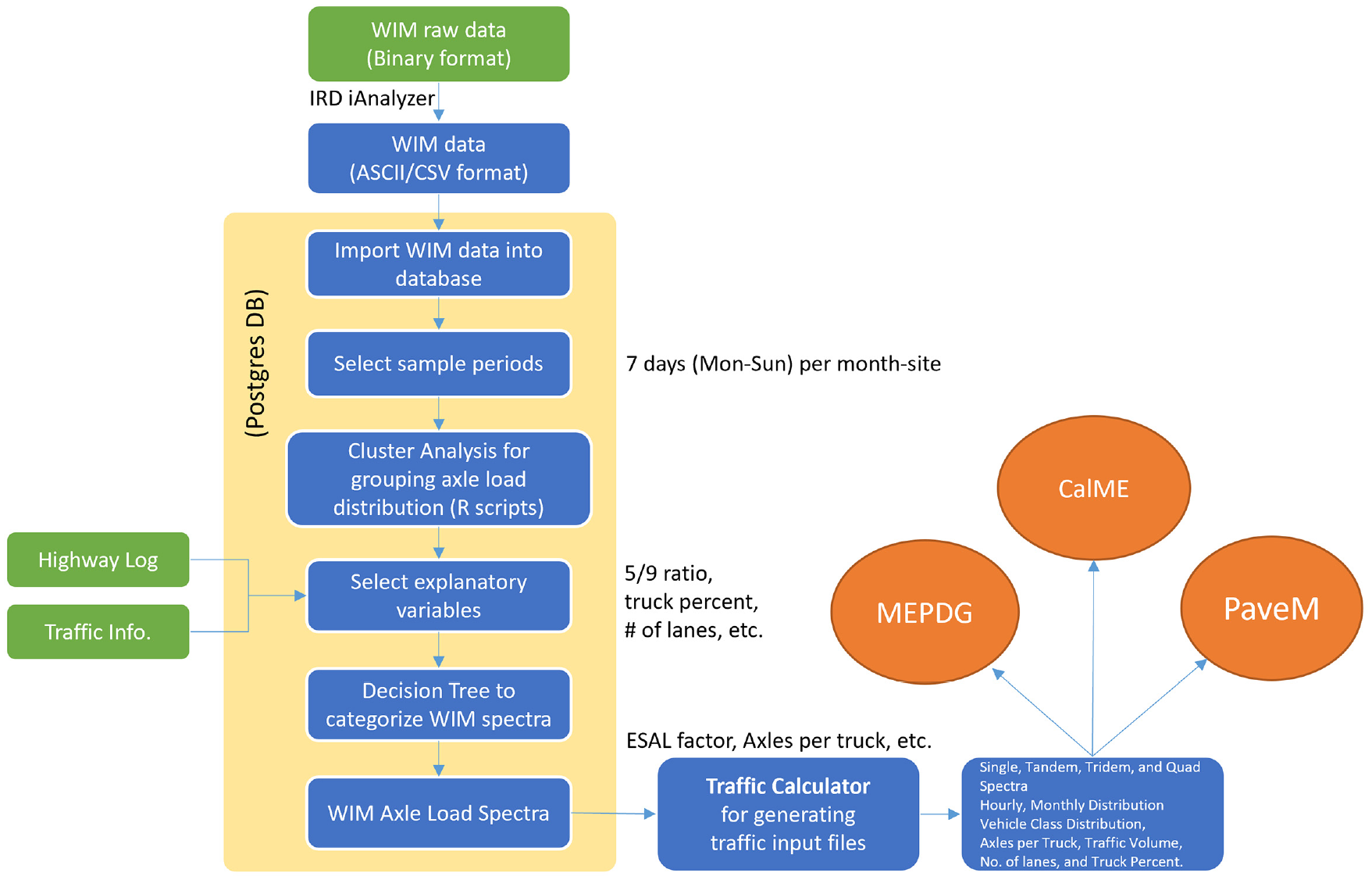
Study flow for updating WIM spectra and implementation. Green boxes: the data sources required for this study; blue boxes: each step for grouping axle load spectra in the study; yellow box: procedure in the PostgreSQL database; orange circles: application tools that use WIM spectra.

Uses of WIM Data in Caltrans Pavement Engineering

Caltrans uses multiple database sources and models in pavement engineering. Caltrans developed various software/applications using those databases and models for pavement design, management, construction analysis, LCA, and life cycle cost analysis. The databases, models, and software/applications interact in Caltrans pavement engineering methods.

WIM data are used for ME pavement design method and LCA in several tools: PaveM, MEDPDG traffic calculator, CalME, and LCA. PaveM is a Caltrans pavement management application developed by UCPRC and uses WIM axle load spectra to calculate pavement performance ( 12 ). MEPDG traffic calculator was developed by UCPRC and uses WIM axle load spectra to generate a set of traffic inputs for running AASHTOWare Pavement ME Design software for rigid pavement design ( 5 ). UCPRC developed CalME for ME pavement design for flexible pavement and takes WIM axle load spectra to determine traffic load in its calculation ( 13 ). UCPRC also developed the LCA application tool that uses WIM axle load spectra as the input parameters in the LCA procedure ( 14 ).

Data Description

WIM Data Acquisition

The WIM data from 2004 to 2015 at all 123 WIM sites were obtained from the Caltrans Office of Commercial Vehicle Operation under the Division of Traffic Operations. The data from the available 80 regular WIM data collection sites were included in the analysis, but the data from 16 PrePass™ sites were excluded from the analysis because of a lack of specific information (i.e., lane numbering). The WIM devices collected one-directional data at 53 sites and two-directional data at 27 sites. Caltrans performed a data quality check each month for each WIM site for proper operation of the WIM system, calibration drift, and proper coding of vehicle records containing questionable data elements. Based on Caltrans’s monthly performance reports, the data that showed good condition in the routine performance check were selected for analysis in this study.

An overview of the California WIM system can be found in the literature ( 2 ). Note that Caltrans implemented the Federal Highway Administration (FHWA) vehicle classification system with slight modifications, adding two more truck classes: class 14 (five-axle truck trailers) and class 15 (irregular trucks and trucks unclassified because of system error).

The Caltrans WIM sites were used to be provided by two vendors: PAT Traffic Control Corporation and International Road Dynamics, Inc. PAT Traffic Control Corporation provided three different systems—DAW 100, DAW 190, and DAW 200—while International Road Dynamics, Inc., provided one system called the IRD system ( 11 ). These two vendors have different data handling software and data formats. Caltrans completely replaced all PAT sites with the IRD system in September 2012. Since then, all California WIM sites have been operated using the IRD system.

Quality of WIM Data

The performance quality of WIM sites in California has significantly improved recently because of the enhancement of communication and calibration technologies. The percentage of days with good quality data in 2004 was only 31%, but the percentage of days with good quality data in 2015 was 85%. The WIM data became much more stable in 2015 than in the previous years. In that sense, it became necessary to reanalyze the axle load spectra with the latest WIM data.

Sample Data Selection

A total of 481,000 binary raw files (185 GB) stored from 123 WIM sites from 2004 to 2014 were converted into two formats of the ASCII files, which were imported into the database (2.5 TB) using iAnalyzer^® software developed by International Road Dynamics, Inc. ( 11 ). One format was the FHWA format, and the other was the Caltrans vehicle classification format. The WIM spectra analysis used the Caltrans format in this study.

Because of the computation time of analysis, the query imported the first seven consecutive days (Monday–Sunday) of each month at each site to the Postgres database. When any missing day was identified among the first seven days of a month, it was replaced with the next day that had good quality data.

WIM Axle Load, Gross Vehicle Weight, and Speed Summary

WIM Axle Load

The axle load spectra of all single axles from the 80 WIM sites were compared between 2005, 2010, and 2015. As shown in Figure 2a, three axle load spectra of the single axle did not show a significant difference. The axle load at 20 kN was the largest proportion (between 25% and 30%), and the axle load at 30 kN was the second largest proportion at 15%. The axle load spectra for 2015 showed a slightly higher proportion at 20 kN but a lower proportion at 70 kN and 80 kN compared with 2005. This indicates that the single axle load in 2015 was slightly lighter than the single axle load in 2005.

Figure 2.

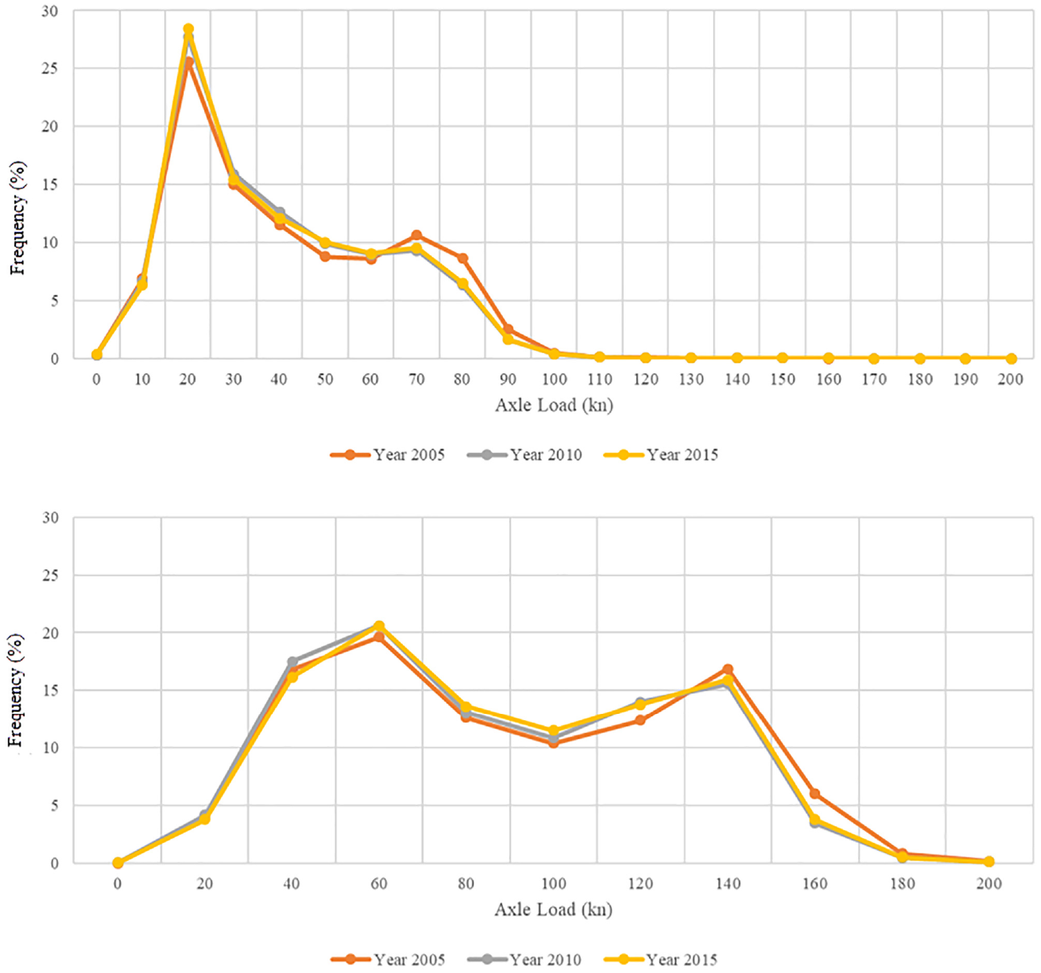
WIM axle load spectra (2005, 2010, and 2015): (a) single axle loads and (b) tandem axle loads.

Figure 2b shows the trend of tandem axle load spectra for the past 11 years (2005, 2010, and 2015). Similar to the single axle load spectra discussed above, the three spectra of the tandem axle loads also showed that the tandem axle load was slightly lighter in 2015 than in 2005. The heavy axle loads (at 140 and 160 kN) decreased slightly, but the light (at 60 kN) and medium (between 80 and 120 kN) axle loads increased.

According to the trends of the axle load spectra in Figure 2, there was no significant change in the truck axle loads for both the single and tandem axles for the past 11 years.

Average Gross Truck Weight

The average gross vehicle weight for each vehicle class was extracted from the WIM database for the same period and analyzed to identify any changes over time. As shown in Figure 3, the average gross vehicle weights of vehicle class 13, consisting of seven or more axles, were the heaviest vehicle class in each year, ranging between 90 and 100 kips. The average gross vehicle weight increased from 94.85 kips in 2005 to 98.81 kips in 2010 and decreased to 91.39 kips in 2015. The lightest gross vehicle weights were observed in vehicle class 5, consisting of two axles, they and showed a narrow range (13.40–13.86 kips), meaning almost no change over time. The average gross vehicle weights of vehicle classes 6, 7, and 8 slightly increased in 2015 compared with 2005. The average gross vehicle weight for heavy vehicles decreased by 3%–4%, whereas the average gross vehicle weights for light and medium vehicles increased by 1%–4% over the past 11 years.

Figure 3.

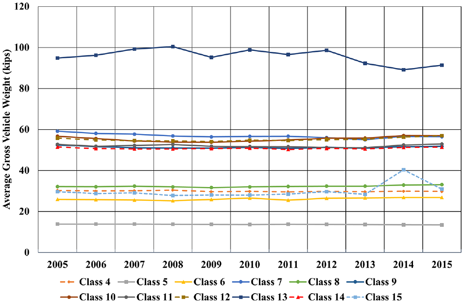
Average gross vehicle weight per vehicle class (2005–2015).

The average gross vehicle weight of vehicle classes 8–14, containing semi-tractor trailers, was 50.13 kips for the analysis periods (2003–2015). About 80% of the heavy vehicles (semi-tractor trailers, vehicle classes 8–14) were found in vehicle class 9, and the average gross vehicle weight for this class was 51.26 kips. It was found that the trend of the average gross vehicle weights over time was consistent with the trend of the WIM axle load spectra over time.

Average Truck Speed

Speed information for heavy vehicles is also valuable for pavement design and analysis. The average speeds of heavy vehicles by vehicle class were calculated each year for the analysis period. Figure 4 shows the average speed change for each vehicle class in all WIM sites from 2004 to 2015. The overall average speed of vehicle classes 5–14 decreased by 11% from 55.8 mph (2004) to 49.7 mph (2015). The average speed for all vehicle classes (classes 5–15) gradually decreased over 11 years. Vehicle class 10 showed the largest decrease in its average speed (16.7%), and vehicle class 12 showed the smallest decrease in its average speed (4.5%) from 2004 to 2015.

Figure 4.

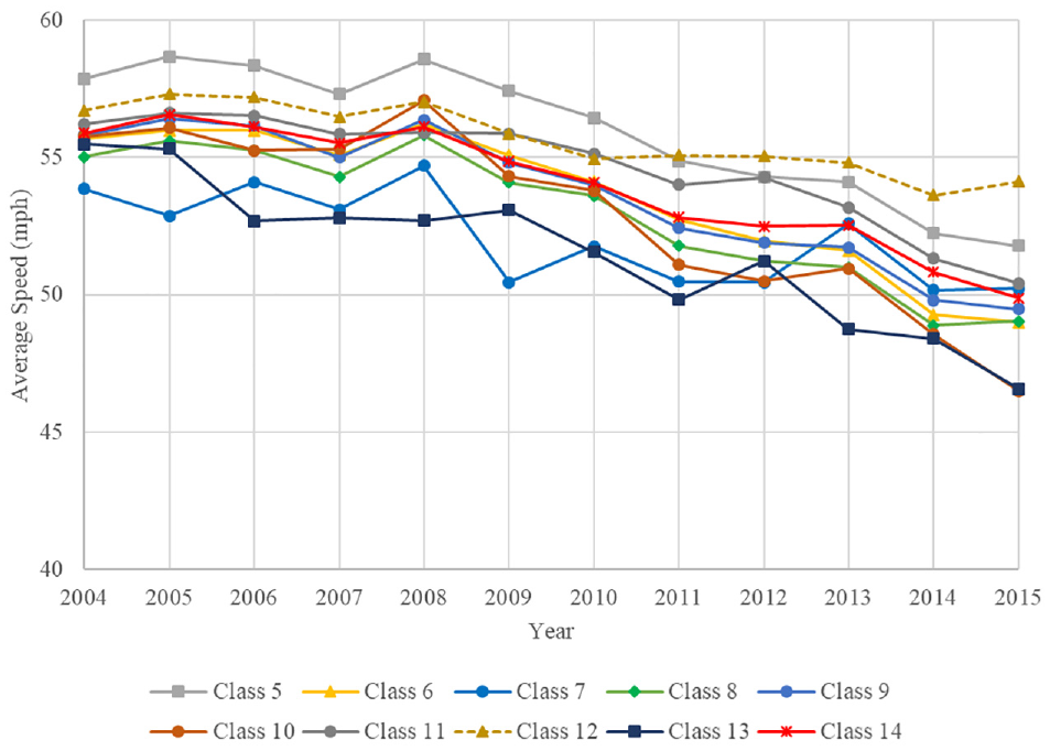
Average speeds of vehicle classes at all WIM sites from 2004 to 2015.

The average speeds of vehicle classes 5, 9, and 13 and vehicle classes 5–15 at each WIM site were compared for 2015. With regard to the average speed for vehicle classes 5–15, 1% of WIM sites showed average speeds <45 mph, and 3% of WIM sites showed average speeds in the range 45–50 mph. Sixty percent of WIM sites showed average speeds in the range 55–60 mph, and 20% of the WIM sites showed average speeds >60 mph. The overall average speed of all WIM sites was 57 mph for vehicle classes 5–15. Vehicle class 5 showed the highest average speed (62 mph), and vehicle class 13 showed the lowest average speed (55 mph) at all WIM sites in 2015.

Methodology

Cluster Analysis with Earth Mover’s Distance Algorithm

The 80 WIM sites were grouped by the similarity of axle load distribution using a hierarchical clustering algorithm in the program R (R Foundation for Statistical Computing, Vienna, Austria). This analysis requires that the “distance” between every pair of samples be computed. The earth mover’s distance (EMD) algorithm was chosen for this purpose because it can use the full axle load distribution. EMD is an efficient algorithm to evaluate dissimilarity between two multidimensional distributions in some feature space ( 15 ). The basic approach in the EMD algorithm is the same as calculating the amount of cut and fill needed to alter a site from the existing profile and the elevations at each station, taught in most basic survey classes in civil engineering. The minimum balance of the entire earth moved takes the shortest time and lowest cost to complete the work. The EMD algorithm is often used in data science fields ( 15 ). In the hierarchical cluster analysis, the distance between each pair of WIM stations was computed by taking the square axle loads as horizontal distance and the cumulative axle load distribution as the land surface profile. Before this could be done, the tandem and tridem axles had to be converted to single axles by halves and thirds of the loads and doubling/tripling the number of axles, respectively. The full distance matrix is passed to the hierarchical clustering algorithm, which recursively finds the nearest pair of distinct clusters and merges them into one group. This is repeated until the number of clusters reaches a single cluster, and the hierarchy of clusters is returned as a tree structure.

Analysis Results

The cluster analysis grouped the 80 WIM sites into seven groups (groups A–G). Group A includes one WIM site that shows the lightest axle load spectra, and group G includes one WIM site that shows the heaviest axle load spectra, as shown in Figure 5. The y-axis shows the distance between a pair of properties, and the higher distance indicates the larger dissimilarity between two properties (groups).

Figure 5.

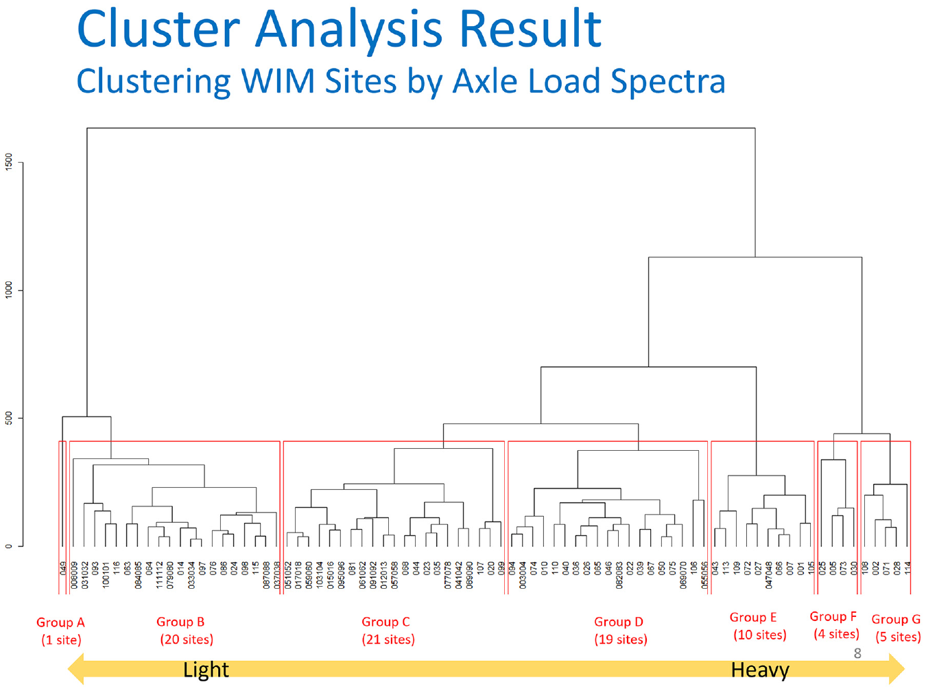
Cluster analysis result (groups A–G).

One WIM site located on Route 49 in district 3 was in group A, and 21 WIM sites in multiple districts were in group C. Group G contains five WIM sites in districts 2, 3, 6, and 8.

Figure 6 illustrates the orders of the WIM sites by the ESALs per 1,000 axles to show the distribution of the WIM groups by the ESALs. Groups A and B, which contain the lighter axle load spectra, were mostly shown below 200 ESALs per 1,000 axles, and groups F and G, which contain the heavier axle load spectra, were mainly shown above 330 EASLs per 1,000 axles. The plot of the WIM sites in the order of ESALs per 1,000 axles shows the consistency of WIM grouping results. It was possible to group WIM spectra only based on ESALs of WIM sites, but the EMD algorithm compares a pair of the axle load distributions of two WIM sites, not just the axle loads.

Figure 6.

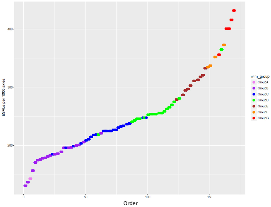
Equivalent single axle loads (ESALs) per 1,000 axles.

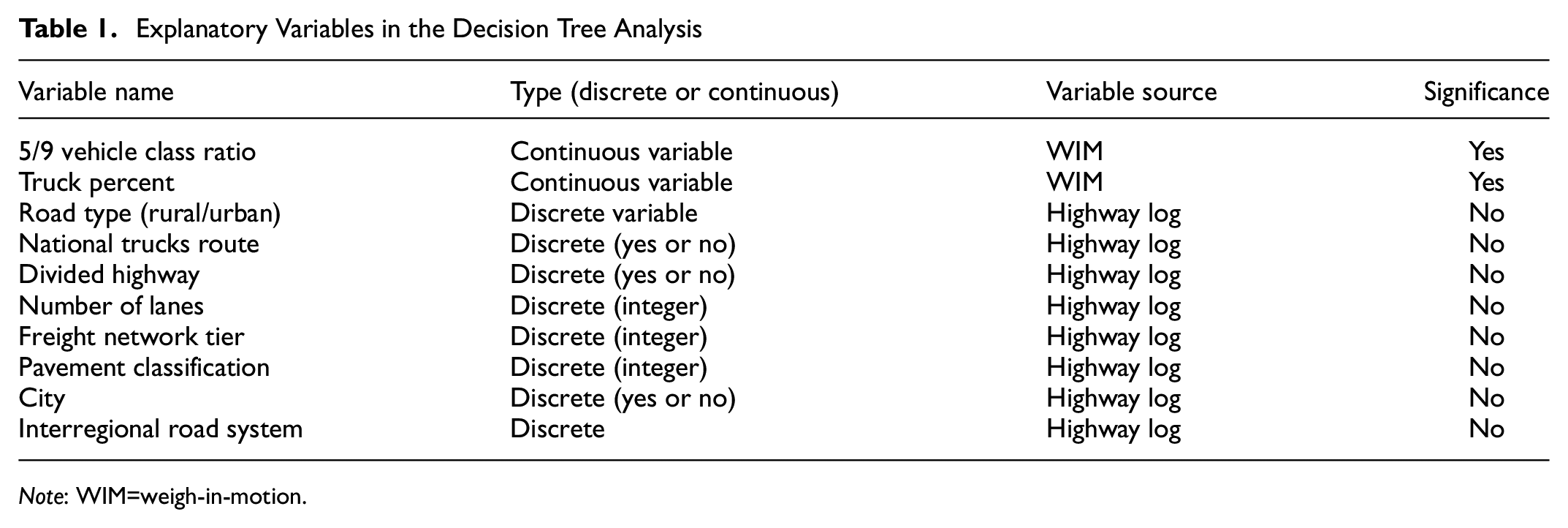
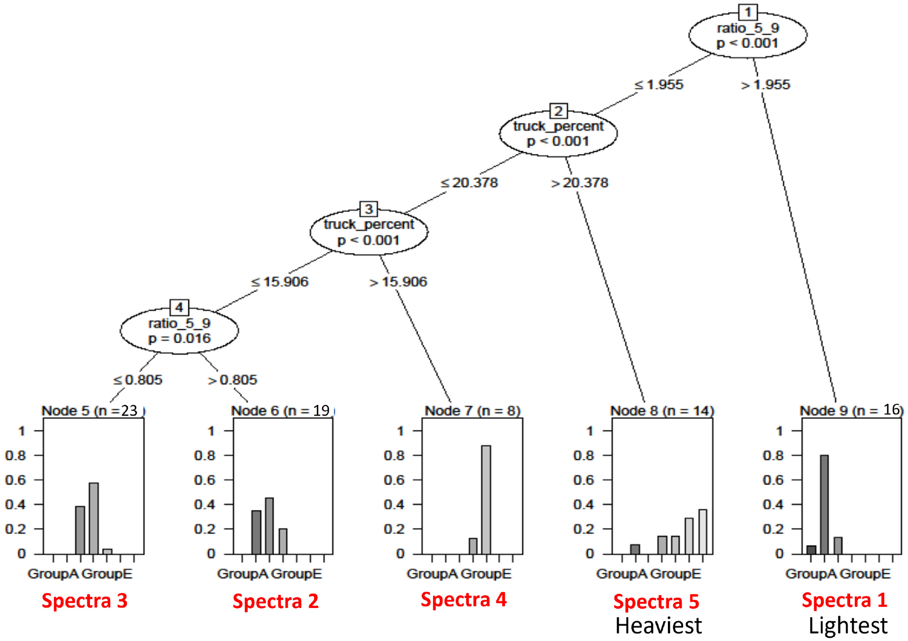
The decision tree model was developed in the program R to group the 80 WIM sites into five WIM spectra by axle load distribution. In developing the decision tree model, several traffic information was extracted from the highway log database in California and the WIM database, and they were considered the explanatory variables. Table 1 shows the explanatory variables included in the decision tree model and their descriptions. According to the decision tree model, two explanatory variables—the ratio of vehicle class 5 to vehicle class 9 (5/9 vehicle class ratio) and truck percent—were statistically significant, but the other variables from the highway log were insignificant. The final decision tree model used those two significant variables to group the WIM sites into five WIM spectra, as shown in Figure 7.

Table 1.

Explanatory Variables in the Decision Tree Analysis

Variable name	Type (discrete or continuous)	Variable source	Significance
5/9 vehicle class ratio	Continuous variable	WIM	Yes
Truck percent	Continuous variable	WIM	Yes
Road type (rural/urban)	Discrete variable	Highway log	No
National trucks route	Discrete (yes or no)	Highway log	No
Divided highway	Discrete (yes or no)	Highway log	No
Number of lanes	Discrete (integer)	Highway log	No
Freight network tier	Discrete (integer)	Highway log	No
Pavement classification	Discrete (integer)	Highway log	No
City	Discrete (yes or no)	Highway log	No
Interregional road system	Discrete	Highway log	No

Note: WIM=weigh-in-motion.

Figure 7.

Result of the decision tree model of WIM Spectra.

The first cut in the decision tree model occurred by the 5/9 vehicle class ratio. The decision tree model separated the WIM sites, where the 5/9 vehicle class ratio was larger than 1.96, from the rest of the WIM sites and grouped them into spectra 1. Spectra 1 is the WIM spectra that show the lightest axle load distribution. In the second decision, the variable (truck percent) functioned to separate the WIM sites for spectra 2 from the rest of the WIM sites. The WIM sites where the truck proportions were larger than 20.38% fell into spectra 2, which showed the heaviest axle load distribution. The truck percent variable was used again in the third discernment of the decision tree method. The WIM sites whose truck proportions were between 15.91% and 20.38% fell into spectra 4. The last decision was made by the 5/9 vehicle class ratio again. The WIM sites, where the 5/9 ratios were between 0.81 and 1.96, were grouped into spectra 2, and the rest of the WIM sites were grouped into spectra 3. The numbers in the spectra names were named by the pattern of axle load distribution on each spectra (where 1=the lightest axle load distribution and 5=the heaviest axle load distribution).

As shown in Figure 8, WIM spectra 1, the lightest axle load spectra, consists of 1, 12, and 3 WIM sites from groups A, B, and C, respectively (total 16 WIM sites), while WIM spectra 5, the heaviest axle load spectra, consists of 1, 2, 4, and 5 WIM sites from groups B, D, E, F, and G, respectively (total 14 WIM sites). WIM Spectra 3 showed the medium axle load spectra, which was observed most often on highways in California and consisted of 10, 12, and 1 sites from groups C, D, and E, respectively (total of 23 sites).

Figure 8.

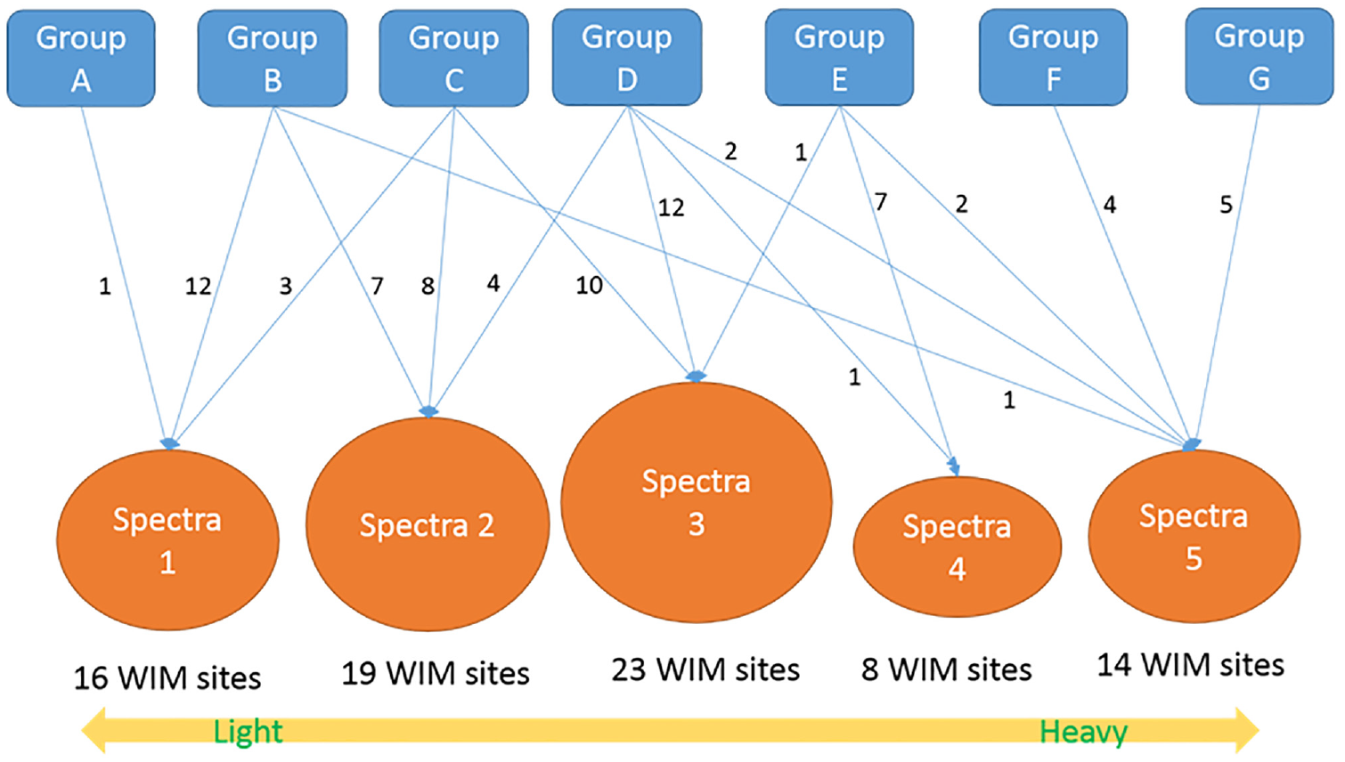
The WIM spectra result in the decision tree model.

Spectra 1, the lightest axle load spectra, included the WIM sites on rural and interregional highway sections in districts 1, 3, 4, 5, 6, 7, 8, 10, and 11 (note that no WIM site existed in district 9). Spectra 2 and 3 (the medium axle load spectra) included the WIM sites on urban and intra-regional highway sections in districts 3, 4, 5, 6, 7, 8, 10, 11, and 12. In particular, none of the 19 WIM sites included in spectra 2 were located in districts 1, 2, 6, and 9, and 22 out of 23 WIM sites in spectra 3 were located on the urban highway sections in districts 3, 4, 5, 6, 7, 8, 10, 11, and 12 (except one WIM site in district 6). This implies that spectra 2 and 3 are the typical axle load spectra that are only overserved on urban highway sections. Spectra 5, the heaviest axle load spectra, were often observed on Interstate 5 in districts 2, 3, 6, and 10 and Interstates 10 and 40 in district 8; the routes function as the interregional major corridors.

WIM Spectra

The decision tree model resulted in five typical WIM spectra. Spectra 1 is the lightest axle load distribution, where the highest proportion (50%) the single-counted axle loads is between 20 and 30 kN. Spectra 2 is the second lightest axle load distribution, where the majority of the single-counted axle loads (about 65%) are concentrated between 20 and 40 kN. Spectra 3 is the medium axle load distribution, where 70% of the single-counted axle loads are widely distributed between 20 and 50 kN, but the proportion of the light axle loads (20 kN) is still slightly higher than the proportion of the heavy axle loads (60 kN). Spectra 4 is the second heaviest axle load distribution, where the axle loads are fairly distributed from 15 kN to 70 kN between 10% and 20%. The proportion of the single-counted axle load at 20 kN is about the same as the proportion of the single-counted axle load at 50 kN. Figure 9 shows the axle load distribution of each axle type for five-axle load spectra.

Figure 9.

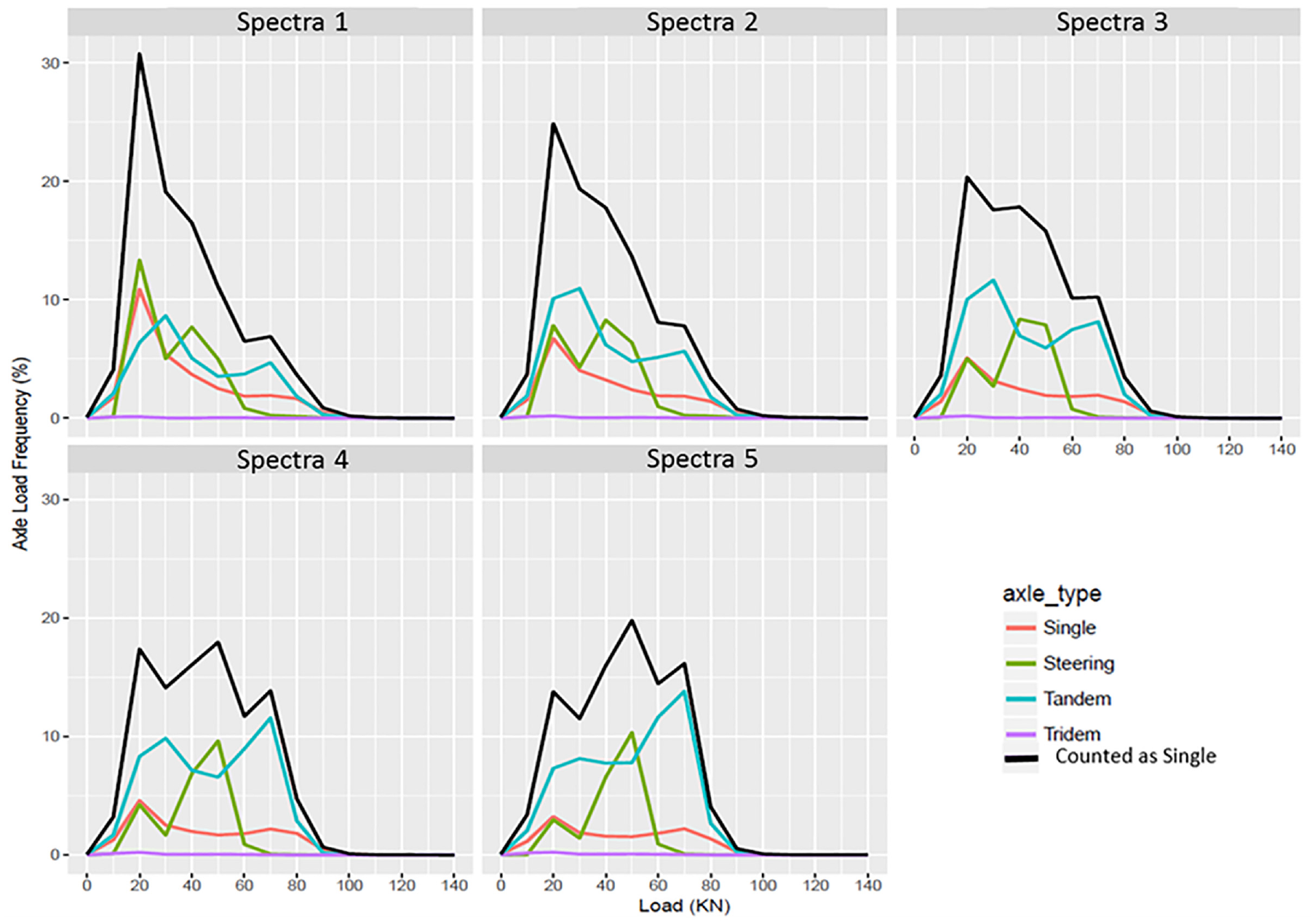
Axle load distributions for five-axle load spectra.

Extension to the Entire Caltrans Network

With the cut tree to determine the spectra in hand, the methodology needed to be extended to any other location on the highway network. This required the truck percentage and 5/9 ratio to be determined for the entire network. In addition, to be useful for predicting design ESALs and other traffic parameters for design and management, the average annual daily traffic (AADT) at all locations on the network needed to be determined. Three sets of data were available for this task: the AADT data from the PeMS, the truck data (CalTrucks), and the AADT from Transportation Systems Network (TSN) in Caltrans. The PEMS data, which only have AADT, are based on raw loop detector/microwave radar counts at 39,000 individual detectors on the network and do not have full coverage. However, raw data should be close to ground truth values at the detectors ( 16 ). The CalTrucks and TSN AADT data are the outputs from a single source, known as the Traffic Census program, which is not well documented. The CalTrucks data consist of AADT, average annual daily truck traffic (AADTT), and the percentages of the various two-, three-, four-, and five-axle trucks, which are published annually on the Caltrans website ( 17 ).

These data consist of a set of points on the network with back and ahead counts at each point. The spreadsheet has almost complete network coverage, missing only some very small segments and the suffixed routes. If the measurement point was not at the start or end of a continuously drivable route segment, the data were extrapolated back or forward to cover the route. Otherwise, the data were extrapolated linearly between the ahead values from one point to the back values at the following point.

The TSN AADT is also produced by the Traffic Census program but is stored annually in the TSN database. The TSN database also stores the history of the Caltrans highway network and is used to extract a snapshot of the network on a particular date. This becomes the “highway log” for the purposes of managing the network and is used by Caltrans’ Geographic Information Systems group to determine the linear reference system (LRS) for a particular year. This is updated annually, allowing one to translate between map coordinates, driven distances, and Caltrans post miles (the official position measures on the network). Because the LRS provides a snapshot of the network at a given time, it is always possible to determine which records in the TSN data were used to develop the LRS.

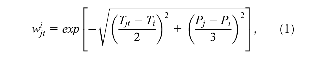
All of these AADT values are the total for both directions, except when the road is unidirectional, and so most need to be halved to determine the AADT in only one direction. This process is performed first. Because they are produced by process of some sort and are not raw data, the TSN AADT values have full network coverage. However, there appear to be some bugs in the process. So, some locations receive AADT counts that are zero or otherwise unrealistic. For this reason, they cannot be used directly. To compensate, the AADT counts from the PEMS data and the full historical AADT counts from the TSN data are imported for every TSN segment in the LRS. A weighted average AADT for every center point of every segment in the LRS is determined from the PEMS data (which is at a point) and all of the historical TSN data both for the segment and the adjacent segments. The weight is based on the following formula:

$$w_{\mathrm{jt}}^i=\exp [-\sqrt{{\left(\frac{T_{\mathrm{jt}}-T_i}{2}\right)}^2+{\left(\frac{P_j-P_i}{3}\right)}^2}],$$

(1)

where $w_{\mathrm{jt}}^i$ is the weight for the $i\mathrm{th}$ segment at time $t$ in the computation for segment $i$ , $T_{\mathrm{jt}}$ is the time of the AADT for the $j\mathrm{th}$ segment at time $t$ (in years), $T_i$ is the time of the AADT for the $i\mathrm{th}$ segment in the LRS, $P_{\mathrm{jt}}$ is the center position of the $j\mathrm{th}$ segment (in miles), and $P_i$ is the center position of the $i\mathrm{th}$ segment in the LRS (in miles).

The weight is thus based on the “distance” of the AADT measurements both in space and time from the segment in question. The weighted mean and weighted standard deviation for the data at each segment are computed and compared with the TSN AADT for the segment at the time of the LRS. If the TSN AADT is zero or has more than two standard deviations from the weighted average, the TSN AADT is replaced with the weighted mean. The value is also rounded using the following formula:

$$\mathrm{AADT}=\frac{\mathrm{round}\left\{200\frac{\mathrm{ADT}}{{10}^{\mathrm{floor}[\mathrm{lo}{\mathrm{g}}_{10}\left(\mathrm{AADT}\right)+1]}}\right\}}{200}{10}^{\mathrm{floor}\left[\mathrm{lo}{\mathrm{g}}_{10}\left(\mathrm{AADT}\right)\right]+1},$$

(2)

where the floor function rounds down to the nearest integer. This effectively rounds to the nearest 1/200th but with only three significant digits (so 196,235 rounds to 195,000). This is the formula used by the Traffic Census program to round the AADT data.

This process identifies around 50 locations on the network where the TSN AADT data in the LRS snapshot are incorrect and replaces them with the average. The percent trucks and percentage of each of the different axle count trucks are linearly interpolated, or if these data are missing in the CalTrucks data, they are replaced with suitable values based on expert judgment. With these data, it is then possible to determine the appropriate WIM spectrum, and with the AADT, any other traffic information for design or management can be determined for every segment on the network.

Final Results for the Entire Caltrans Network

The new WIM spectra developed in the decision tree model were applied to the highway network in California, and the results are shown in Figure 10. Each pavement segment was classified into one of the five WIM spectra based on its vehicle class 5/9 ratio and truck percentage. The R script used two variables to determine WIM spectra for each pavement segment.

Figure 10.

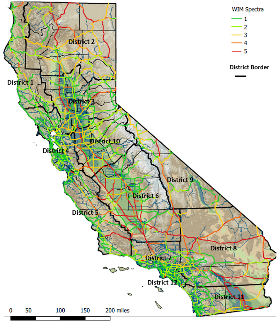
Display of applying WIM spectra to the highway network in California.

The pavement segments are divided by highway characteristics such as the number of lanes changes, on-/off-ramp, the bridge begins/ends, and so on. Most segments on the Interstate 5 corridor are classified into spectra 5, the heaviest axle load distribution, and most segments on highway 1 fall into Spectra 1, the lightest axle load distribution. Urban highways in districts 3, 4, 7, 8, 12, and 11 turn out to have light or medium axle load distribution, which are shown in spectra 1, 2, and 3, whereas rural highways in districts 2, 3, 4, and 8 fall into spectra 4 and 5.

Application Tool for ME Pavement Design

Scope and Purpose of the Application Tool Development

The UCPRC developed MEPDG Traffic Input Process (MEPDG-TIP) for Caltrans to generate a set of traffic-related inputs required for running ASSHTOWare Pavement ME Design software (previously called MEPDG) for pavement design with ME methodology. The main traffic input for ASSHTOWare Pavement ME Design is the axle load spectra by WIM groups, and the five WIM spectra representing typical axle load spectra in the highway network in California were incorporated into the tool. Using MEPDG-TIP, users can quickly prepare necessary traffic input data for the project-specific location to run ASSHTOWare Pavement ME Design software in the pavement structure design.

MEPDG-TIP decides the WIM spectra of the project site based on user inputs (district, county, route, direction, and post mile) and shows the axle load spectra for each month (January–December) and each vehicle class (4–14) for the corresponding WIM spectra, hourly distribution, monthly distribution, vehicle class distribution, axle per truck type (single, tandem, and tridem axles), and traffic volume in the “MEPDG Traffic Inputs” window. The quad axle is excluded in MEPDG-TIP because it is not often observed in California. Figure 11 illustrates the process of MEPDG traffic input generation in MEPDG-TIP.

Figure 11.

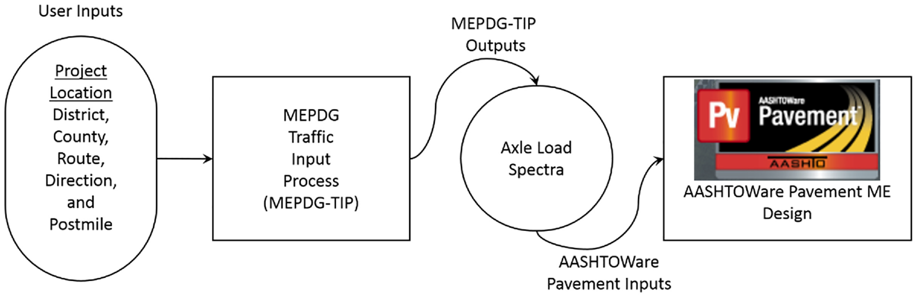
Process of the traffic calculation tool, Mechanistic–Empirical Pavement Design Guide Traffic Input Process (MEPDG-TIP).

After reviewing the output results in the “MEPDG Traffic Inputs” window, a user can export the MEPDG-TIP outputs as the input formats of ASSHTOWare Pavement ME Design to the selected folder.

Outputs

The “MEPDG Traffic Inputs” window contains nine tabs:

1. Single axle spectra: single axle spectra for truck class for each month.

2. Tandem axle spectra: tandem axle spectra for truck class for each month.

3. Tridem axle spectra: tridem axle spectra for truck class for each month.

4. Quad axle spectra: quad-axle spectra for truck class for each month. (This tab is empty because quad axle trucks are rarely operated in California. Thus, quad axle spectra information is not achievable. However, the ASSHTOWare Pavement ME Design software still requires the quad axle spectra information.)

5. Hourly distribution: traffic distribution for hour of day.

6. Monthly distribution: monthly distribution is not created from the WIM data in MEPDG-TIP v1.5.

7. Vehicle class distribution.

8. Axles per truck: number of axles per truck class.

9. Traffic volume and other inputs: two-way AADTT, number of lanes in design direction, percent of trucks in design direction, and ESALs per 1,000 trucks.

The MEPDG traffic inputs in the traffic calculation tool can be exported to the MEPDG traffic input files, which are readable in the ASSHTOWare Pavement ME Design software by clicking the button on the main window. The six files generated in the chosen folder can be imported into the ASSHTOWare Pavement ME Design software.

Concluding Summary

WIM Spectra

California’s representative axle load spectra were developed by the cluster analysis with the decision tree method from the latest WIM data set (2004–2015) collected at 107 WIM sites (53 one-directional and 27 two-directional sites) across the highway in California. The cluster analysis resulted in seven WIM groups based on axle load distribution between the WIM sites. The decision tree method resulted in five WIM spectra, with the truck percentage and the vehicle class 5/9 ratio as the critical explanatory variables to determine WIM spectra. Spectra 1 consists of the lightest axle load distribution observed in 16 WIM sites. Spectra 2 consists of the second lightest axle load distribution found in 19 WIM sites. Spectra 3 shows the medium axle load distribution, and it is the most popular type, shown in 23 of 80 WIM sites in California. Spectra 4 is the second heaviest axle load spectra observed in eight WIM sites. The heaviest axle load spectra, spectra 5, is observed in 14 WIM sites. The updated WIM spectra in this study were applied to the highway segments based on each truck percentage and vehicle class 5/9.

Traffic Calculation Tool

In this study, as an application of the WIM axle load spectra, the traffic calculation tool was developed to generate input files for the ME pavement design software, ASSHTOWare Pavement ME Design. This tool determines WIM spectra for the chosen pavement route and post mile and generates the corresponding input files required in ASSHTOWare Pavement ME Design. The generated input files can be directly imported into ASSHTOWare Pavement ME Design. This helps pavement engineers to use the appropriate input files in their ME pavement design.