Sage Journals: Discover world-class research

Abstract

This study investigated the effects of moderate daily temperature variations on reflective cracking in asphalt concrete (AC) overlays on Portland cement concrete (PCC) pavements using three-dimensional (3D) finite element (FE) modeling. The FE model consists of an AC overlay on top of PCC slabs, followed by aggregate base and subgrade. The year-round temperature variations were divided into discrete groups using a clustering technique and each group was applied separately in the FE model. The maximum stress and strain values associated with each temperature variation group were determined using the FE model and used as the driving force corresponding to the thermally induced damage in the AC overlay. The results show that the maximum stress and strain values in the overlay depend on the hourly temperature variation as well as the seasonal temperature profile. The daily temperature variation controls the deformation of the underlying PCC slabs, whereas the seasonal temperature profile determines the viscoelastic properties of the AC overlay. The estimated maximum tensile stress and strain values suggest that the AC overlay is primarily subjected to damage from repetitive thermal loading instead of one-time fracture events for moderate temperature variations. In addition, when the AC overlay is fully bonded to the PCC slabs, the thermal strains are much greater than the traffic induced strains, indicating a high possibility of thermal reflective cracking being the dominant damage mechanism for these cases.

Keywords

infrastructure pavements design and rehabilitation of asphalt pavements mechanistic–empirical pavement design pavement distress pavement modeling pavement performance modeling

The effects of temperature variation on reflective cracking in asphalt concrete (AC) overlays on Portland cement concrete (PCC) pavement can be divided into two types: one-time cracking events caused by severe temperature drops, and thermal fatigue cracking caused by moderate daily temperature variations. The former occurs at low temperatures combined with severe and rapid cooling events which result in high tensile stresses at the surface of the AC overlay that exceed the tensile strength of the AC used. By contrast, the latter does not require low temperatures. The thermal stress in the AC overlay is caused by the expansion–contraction cycles of the joints and/or cracks in the underlying PCC layer and remains lower than the strength. As a result, the thermal damage gradually accumulates in the AC overlay as the number of thermal expansion–contraction cycles increases. The likely critical parameters for expansion and contraction are the magnitude of the daily temperature fluctuations at the interface between the overlay and the underlying layer, as well as the yearly maximum and minimum temperatures found at the same location ( 1 ). Many experimental tests and numerical models ( 2 , 3 ) have been developed to evaluate the one-time cracking behavior of AC materials. However, limited research can be found concerning the impact of the daily-temperature-variation-induced movement of the underlying layer on the stress and strain condition in the AC overlay.

Daily temperature variation has been argued to have more impact on the reflective cracking of the AC overlays than traffic loads, especially for semi-rigid pavements ( 4 ). Several observations on thermal fatigue cracking caused by the movements of the underlying layers in the field have been reported. In west Texas, where moderate temperatures prevail, extensive amounts of transverse cracking in the asphalt layer have been observed ( 5 ). In addition, a field measurement study of pavement strain in Virginia revealed that the highest strain in the AC layer was detected on April 16 when the largest temperature gradient occurred instead of when the lowest temperature was observed ( 6 ), implying that the critical strain in the AC overlay is a function of the temperature gradient and is not necessarily related to the lowest pavement temperature.

To quantify the impact of temperature variation, Epps ( 7 ) conducted fatigue tests by subjecting beam specimens to flexural fatigue loading at a temperature of 4°C and a loading frequency of 0.05 Hz. The applied tensile stresses to cause thermal fatigue failure were determined based on the extreme cases of thermal events calculated using the COLD program ( 8 ), which is normally used to predict low temperature cracking, and tensile strengths obtained from indirect tension tests. From this study, a linear correlation was found between the thermal fatigue life and the stress level applied. To predict the thermal fatigue life, accurate estimation of thermal strain from stiffness for the temperature and load frequency and applied stress is critical. Finite element (FE) modeling has been proven accurate in predicting thermal strain in pavements. A study showed that the simulated strain values from FE modeling was close to the ones measured in the field with approximately 6% in difference ( 9 ). The recently updated reflective cracking model in the mechanistic–empirical pavement design guide (MEPDG, now called Pavement ME) has incorporated the thermal stress obtained from FE modeling simulations into the cracking propagation model with the Paris’ law from fracture mechanics ( 10 ).

For estimating thermal responses, the viscoelasticity of the AC overlay must be accounted for properly. This makes most traffic-induced reflective cracking models unsuitable because they tend to treat AC as linear elastic. It is expected that thermal responses in AC overlays will depend on loading time and temperature.

To accurately model reflective cracking, the effect of daily temperature variations should be taken into consideration. This paper focuses on AC overlays over PCC slabs and uses FE modeling to predict critical responses under thermal loading caused by moderate daily temperature variations. The term “moderate temperature variation” in this study refers to these temperature variations not drastic enough to cause a low temperature cracking but sufficient to lead to fatigue cracking at moderate climate regions. The results will be used to provide insight into the mechanisms of thermal reflective cracking and can be used for future development of a thermal fatigue damage model.

FE Model for Thermal Loading

The composite pavement structure in the FE model consisted of an AC overlay, PCC slabs separated with joints without dowels, and a layer with finite thickness under the PCC slabs representing both the base and subgrade layer. The joints were introduced to the model not only to describe the load transfer between slabs but also to prevent overlapping between slab corners during the simulation. Detailed information concerning the construction of the numerical model and validation is provided here.

FE Model Information

Model Geometry and Boundary Condition

The FE model was developed based on a selected section from a heavy vehicle simulator (HVS) test track at the University of California Pavement Research Center (UCPRC) ( 11 ) as highlighted in Figure 1. The asphalt material used in the AC overlay for the selected section 2 of Lane B includes a polymer modified binder (PG64-28 PM).

Figure 1.

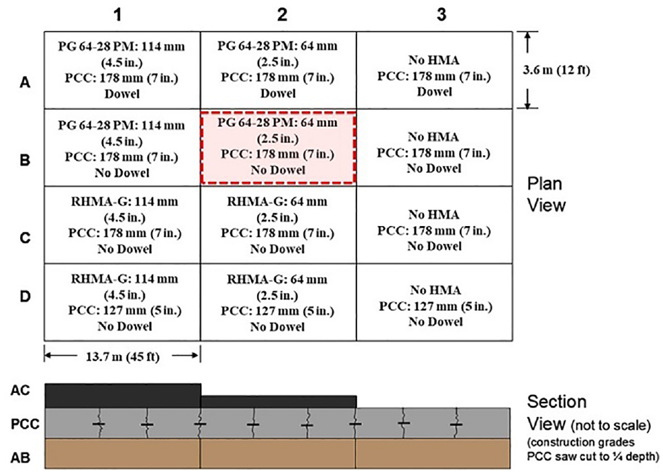
Test track sections with the selected Lane B section 2 for finite element (FE) modeling.

The dimensions of the FE model are the same as the ones shown in Figure 1 with the AC overlay thickness of 64 mm, PCC thickness of 178 mm and the combined aggregate base and subgrade (AB+SG) thickness of 4 m. When the thickness of AB+SG layer increases, the stress and strain in the upper layers (AC overlay and PCC slabs) tend to decrease. The thickness of 4 m was determined based on a sensitivity study with various AB+SG thickness, where no significant change was found in the pavement responses when the AB+SG thickness was above 4 m. The PCC layer consists of three slabs separated by undoweled transverse joints. The joint between the PCC slabs can be modelled with different approaches: empty spaces between PCC slabs ( 12 , 13 ), elements with low stiffness ( 14 ) or cohesive elements ( 15 ). In this study, the cohesive zone modeling (CZM) elements (COH3D8) were inserted to simulate the joint between PCC slabs. The CZM was used for the purpose of characterizing the load transfer efficiency (LTE) of the joint by means of shear stiffness of the CZM elements ( 16 , 17 ). Given the symmetry of the structure, only a quarter of the composite pavement was modeled for computational efficiency. The three-dimensional (3D) FE model is illustrated in Figure 2.

Figure 2.

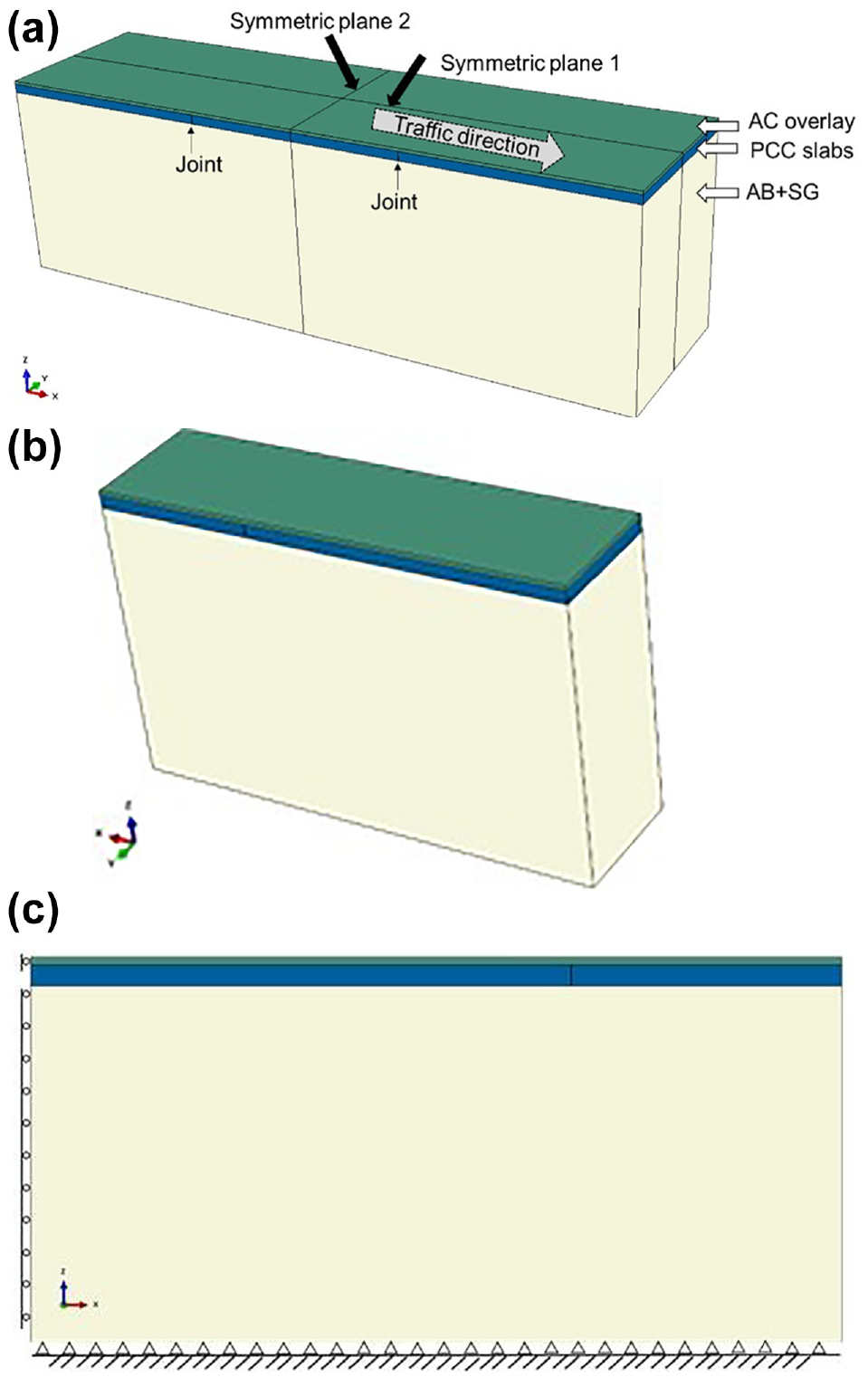
Finite element (FE) model for composite pavement: (a) full model of asphalt overlay on Portland cement concrete (PCC) slabs, (b) one-quarter model, and (c) boundary condition.

Figure 2, a and b , shows the full model of the pavement structure and the corresponding one-quarter structure, respectively. The following boundary conditions have been assigned to the pavement:

(1) As the model was symmetric in both the X and Y directions, symmetric boundary conditions were applied to both the symmetric plane 1 and symmetric plane 2 where the degree of freedom (DOF) perpendicular to the corresponding symmetric plane was constrained.

(2) The AC overlay and the combined aggregate base and subgrade (AB+SG) layer are assumed to be continuous and infinite in the traffic direction. Therefore, the movement along the traffic direction was constrained at the ends of the overlay and the AB+SG layer as shown in Figure 2c.

(3) The side faces of the AC overlay and AB+SG are subject to free movement across the traffic direction.

(4) The boundary condition of encastre (fully built-in) was assigned to the bottom of the AB+SG layer to constrain all degrees of freedom at the pavement bottom.

(5) There is no boundary condition applied on the PCC slabs in the FE model.

Most of the interfaces between parts were set to be fully bonded: the AC overlay was completely tied to the PCC slabs and the vertical surfaces of joints were also fully bonded with the adjacent PCC surfaces. The bottom of the PCC layer was in contact with the AB+SG layer. The contact does not allow penetration or separation in the normal direction but allows frictional sliding in the tangential direction. The AC overlay bottom was set to be fully bonded with the PCC top as it was assumed that no damage occurred to the bonding between the AC overlay and PCC slabs at the early stage of the pavement given proper construction.

Material Property

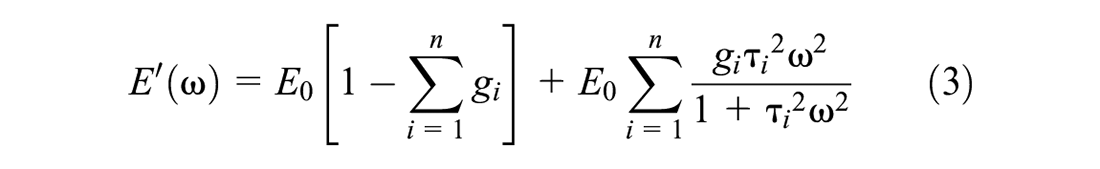
The AC overlay was modeled as a viscoelastic material, whereas the PCC slabs and the AB+SG layer were treated as linear elastic materials to capture the strain caused by hourly temperature change in the pavement. The generalized Maxwell model (GMM) was used to describe the viscoelastic Young’s modulus of the AC overlay, which was mathematically approximated by the Prony series in ABAQUS. The GMM consisted of N different Maxwell units in parallel, each unit with different parameter values. The Poisson’s ratio of the AC layer is assumed to be constant.

In general, the more elements one model has, the more accurate it can be in describing the response of real materials. The viscoelastic constitutive model of the GMM can be mathematically represented by Equation 1:

σ = E_{\infty} ε + \sum_{i = 1}^{n} σ_{i}^{M}

(1)

where

$E_{\infty}$ = stiffness of the “stand-alone” elastic spring,

n = number of Maxwell elements, and

$σ_{i}^{M}$ = stress in the ith Maxwell element, which is given: $σ_{i}^{M} = E_{i} (ε - ε_{i}^{M}) = \frac{η_{i} \partial ε_{i}^{M}}{\partial t}$ , $E_{i}$ is the stiffness of the elastic spring of the ith Maxwell element.

Equation 1 can also be re-written using the integrating factor $e^{Et / η}$ as Equation 2:

σ = E_{\infty} ε + \sum_{i = 1}^{n} ε E_{i} e^{- \frac{t}{τ}}

(2)

Then the relaxation modulus is defined as: $E (t) = \frac{σ}{ε} = E_{\infty} + \sum_{i = 1}^{n} E_{i} e^{- \frac{t}{τ}}$ , which is essentially the Prony series representation. $E_{\infty}$ is the final (or equilibrium) modulus, and $E_{0} = E_{\infty} + \sum_{i = 1}^{n} E_{i}$ is the instantaneous modulus. A pair of $E_{i}$ and $τ$ is referred to as a Prony pair which can also be related to the storage and loss moduli using the following equations (Equations 3 to 5):

E' (ω) = E_{0} [1 - \sum_{i = 1}^{n} g_{i}] + E_{0} \sum_{i = 1}^{n} \frac{g_{i} {τ_{i}}^{2} ω^{2}}{1 + {τ_{i}}^{2} ω^{2}}

(3)

E ″ (ω) = E_{0} \sum_{i = 1}^{n} \frac{g_{i} τ_{i} ω}{1 + {τ_{i}}^{2} ω^{2}}

(4)

E (ω) = \sqrt{{(E')}^{2} + {(E ″)}^{2}}

(5)

where

$ω$ = angular frequency,

$E' (ω)$ = storage modulus,

$E ″ (ω)$ = loss modulus, and

g_{i} = \frac{E_{i}}{E_{0}} .

In ABAQUS, the Prony series are described with pairs of $τ_{i}$ and $g_{i}$ , which were obtained through fitting the four-point bending (4PB) flexural frequency sweep testing results with Equations 3 and 4. The fitting procedure followed steps proposed in Wu et al. ( 18 ). As the 4PB frequency sweep tests are performed under different temperatures, the reduced angular frequency $ω_{red}$ was introduced to account for the temperature effect on the asphalt viscoelasticity with the Williams–Landel–Ferry (WLF) model. The shift factor $α_{T}$ was calculated with the help of a sigmoidal function as shown in Equation 6:

\log (a_{T}) = - \frac{C_{1} (T - T_{ref})}{C_{2} + (T - T_{ref})}

(6)

where

$C_{1}$ and $C_{2}$ = positive constants,

T = temperature, and

$T_{ref}$ = reference temperature (20°C in this study).

It was found that the first two branches in an eight-branch GMM were not needed as they did not show significant effect on the overall stiffness of the GMM ( 18 ). Therefore, a six-branch GMM was applied to characterize the asphalt viscoelasticity. The fitting of frequency sweep results to the GMM was carried out using the Microsoft Excel Solver by minimizing the root mean square (RMS) between the measured and fitted moduli.

Loose asphalt mixes were collected during the construction for Lane B section 2 to be compacted in the laboratory to perform the 4PB frequency sweep testing. Three testing temperatures—10, 20, and 30°C—were selected. The comparison between the data measured from the frequency sweep testing and fitted results is shown in Figure 3. The value of RMS from the generalized reduced gradient (GRG) nonlinear solver is approximate 0.13. The corresponding Prony series parameters at the reference temperature (20°C) after fitting are given in Table 1.

Figure 3.

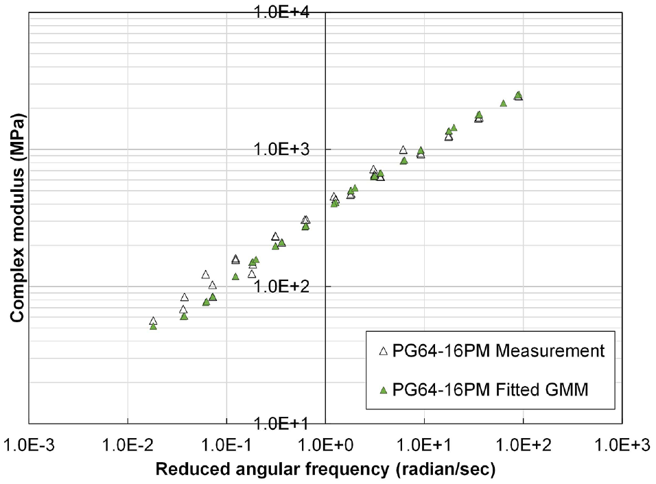
Comparison between frequency sweep testing results and fitted generalized Maxwell model (GMM) results for PG64-16 PM.

Table 1.

Fitted parameter values for generalized Maxwell model (GMM) and Prony series in ABAQUS

Model and variable	Value
GMM
E₁ (MPa)	14,850.1
E₂ (MPa)	1,913.1
E₃ (MPa)	1,049.7
E₄ (MPa)	420.9
E₅ (MPa)	116.5
E_∞ (MPa)	48.2
E₀ (MPa)	18,398.5
Prony series
τ₁	0.0002
τ₂	0.0284
τ₃	0.2172
τ₄	1.6723
τ₅	13.7273
g₁	0.8071
g₂	0.1040
g₃	0.0571
g₄	0.0229
g₅	0.0063
WLF
C₁	25
C₂	200
T_ref (°C)	20

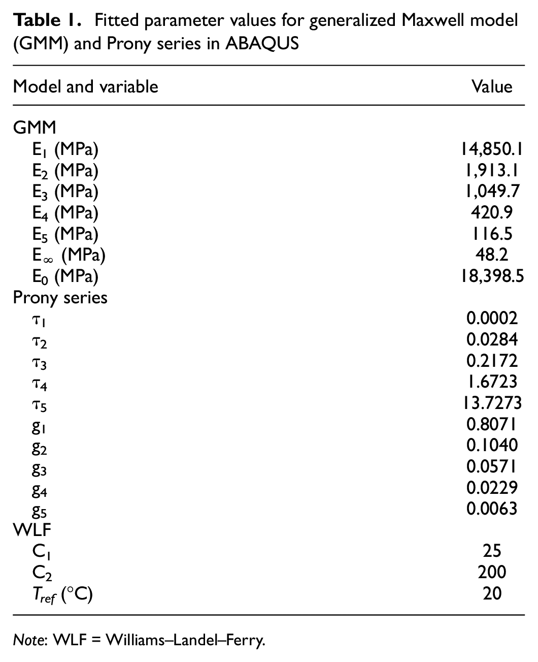
Note: WLF = Williams–Landel–Ferry.

In addition to the viscoelasticity of the asphalt material, other material properties considered in this study include the coefficient of thermal expansion (CTE) for both the AC layer and the PCC slabs, density and Poisson’s ratio for the AC, PCC and AB+SG layers, and the elastic modulus for the PCC slabs and the AB+SG layer. The CTE value of the AC layer was assumed based on experience ( 19 ), and the elastic modulus of the PCC layer was determined through backcalculation using falling weight deflectometer (FWD) data. Meanwhile, the initial CTE value for the PCC slabs in the test sections was measured by laboratory testing on field core samples in accordance with AASHTO TP 60. Typical values of density and Poisson’s were selected for all three layers. The values for these properties are given in Table 2.

Table 2.

Property values for three layers in the finite element (FE) model

Layer	CTE (µε/°C)	Elastic modulus (MPa)	Density (kg/m³)	Poisson’s ratio
Asphalt	20	E ₀ in Table 1	2,600	0.25
PCC	8	48,635	2,500	0.3
AB+SG	na	160	2,200	0.3

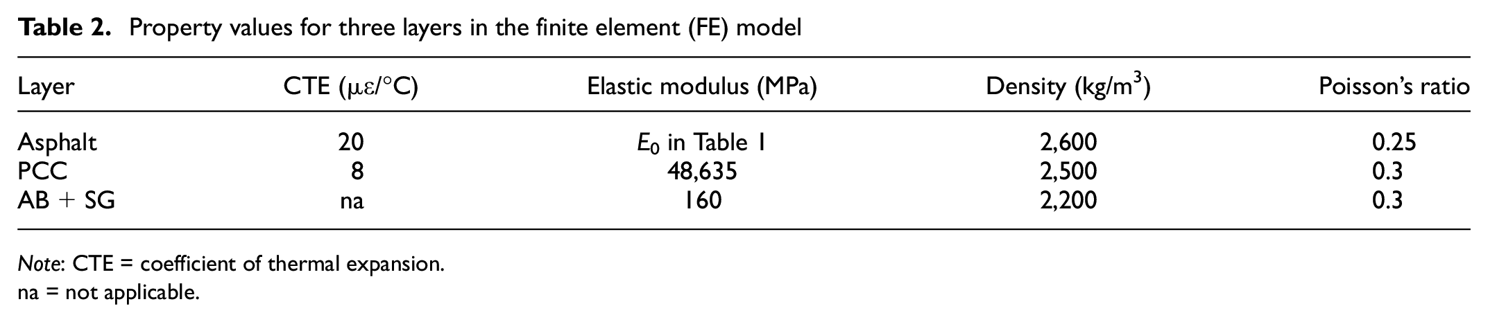
Note: CTE = coefficient of thermal expansion.

na = not applicable.

Loading

To validate the 3D FE model of the AC overlay on top of the PCC slabs, temperature profiles throughout the depth of the AC layer and PCC layer from Section 2 on Lane B were applied as shown in Figure 4, which were measured using thermocouples embedded at different depths in the pavement. The temperature for model validation was selected from 17:00 on January 22 to 16:00 on January 23, 2011. As the PCC layer shows the highest temperature at 17:00, it was assumed that the pavement is at the zero-strain condition at 17:00. To assign the temperature profiles which are dependent on thickness and loading time to the FE model, the AC layer and PCC slabs have been vertically partitioned evenly into three and five sublayers respectively along the depth, and each sublayer was given a uniform temperature that changes with time.

Figure 4.

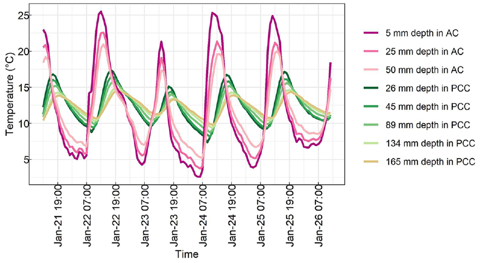
Temperature profile across the depth of asphalt layer and Portland cement concrete (PCC) layer from January 21 to January 27, 2011.

In addition to the thermal loading, a gravitational acceleration of 9.81 m/s² was used to account for the effect of self-weight.

Mesh Convergence

The area in the AC overlay above the joints between PCC slabs is the area of interest in this study. As a result, graded mesh sizes were assigned to the AC layer in the traffic direction with denser mesh near this area and coarser mesh away from the area with sizes ranging from 0.01 m to 0.1 m. A uniform element size of 0.05 m was assigned to the AC overlay along the transversal direction. In the depth direction, the element size was set to be 0.005 m. Concerning the PCC slabs, a biased element size scheme with size from 0.02 m to 0.1 m was applied along the traffic direction. A uniform element size of 0.1 m was assigned to the PCC slabs across the traffic direction, and an uniform element size of approximately 0.01 m was used along the depth direction.

With respect to the AB+SG layer, denser elements with a size of 0.04 m were used in the top area close to the PCC slabs and a larger element size of 0.2 m was set near the bottom along the depth direction. The element type used for the asphalt layer, PCC slabs and AB+SG layer was the 3D 8-node linear brick with reduced integration (C3D8R), and the 3D 8-node cohesive element (COH3D8) was assigned to the joints between two PCC slabs.

A mesh convergence study was carried out to determine the mesh element size for the area of interest (AOI) with a length of 0.1 m at each side of the joint (0.2 m in total) along the traffic direction, as illustrated in Figure 5a with the maximum tensile stress and the strain at the bottom of the AOI as the output variables. Figure 5b demonstrates that both the tensile strain and tensile stress reach a convergence (within 5% difference change) when the element number is 5 and element size of the AOI is 0.005 m. Figure 6 shows the overview of the meshed 3D FE model with a close-up side view.

Figure 5.

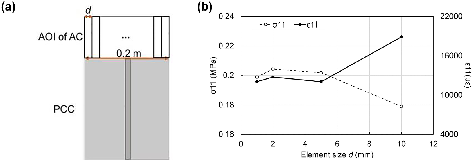
Mesh convergence study with varying element size d: (a) illustration for mesh size d and (b) mesh convergence study result.

Figure 6.

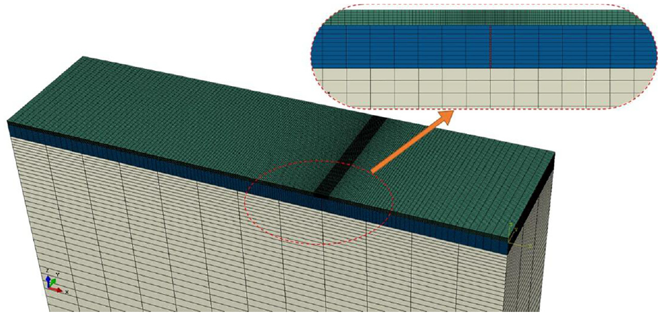
Meshed elements in the three-dimensional (3D) finite element (FE) model.

FE Model Validation

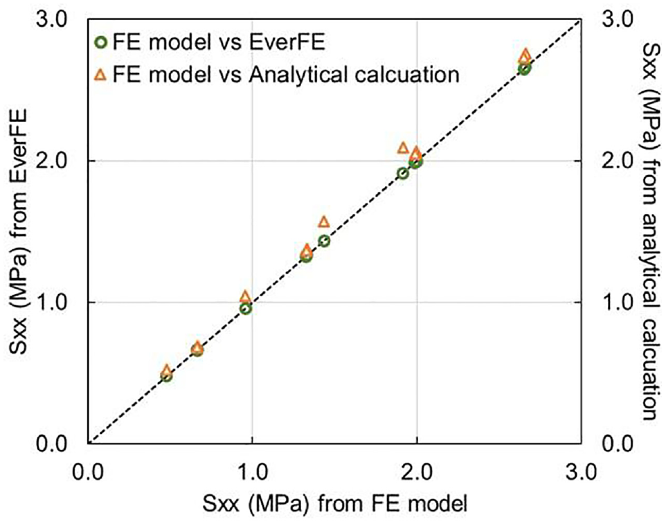
Before validating the FE model simulation results against field measurements, a verification process has been conducted to ensure the FE model is computing correctly and accurately. The stress values in the PCC slabs under temperature change obtained from the FE model were compared with the ones from the software of EverFE ( 20 ) and analytic equations ( 21 ) as shown in Equation 7.

S_{xx} = \frac{E α_{t} Δ t}{2 (1 - v^{2})} (C_{x} + v C_{y})

(7)

where

$S_{xx}$ = total stress along x direction,

E = elastic modulus of concrete,

$Δ t$ = temperature differential between the top and the bottom of the slab,

$α_{t}$ = coefficient of thermal expansion of concrete,

$C_{x}$ and $C_{y}$ are correction factors for a finite lab,

$v$ = Poisson’s ratio of concrete

The comparison of stress in the PCC slabs among the FE model, EverFE, and analytic equation is shown in Figure 7. The various data points represent the PCC slabs with different dimensions. The alignment of these data points reflects that the developed FE model exhibits reasonable output values.

Figure 7.

Verification of finite element (FE) model against EverFE and analytic equation.

The validation of the FE model was conducted by comparing the simulated joint movements against the measured data collected from the HVS test section (see Figure 8). The maximum horizontal movements of both measured and simulated values occur when the temperature at the PCC surface is the lowest. As for the vertical movement, the highest movement coincides with the largest temperature difference between the PCC surface and PCC bottom (temperature gradient) which contributes to the curling deformation.

Figure 8.

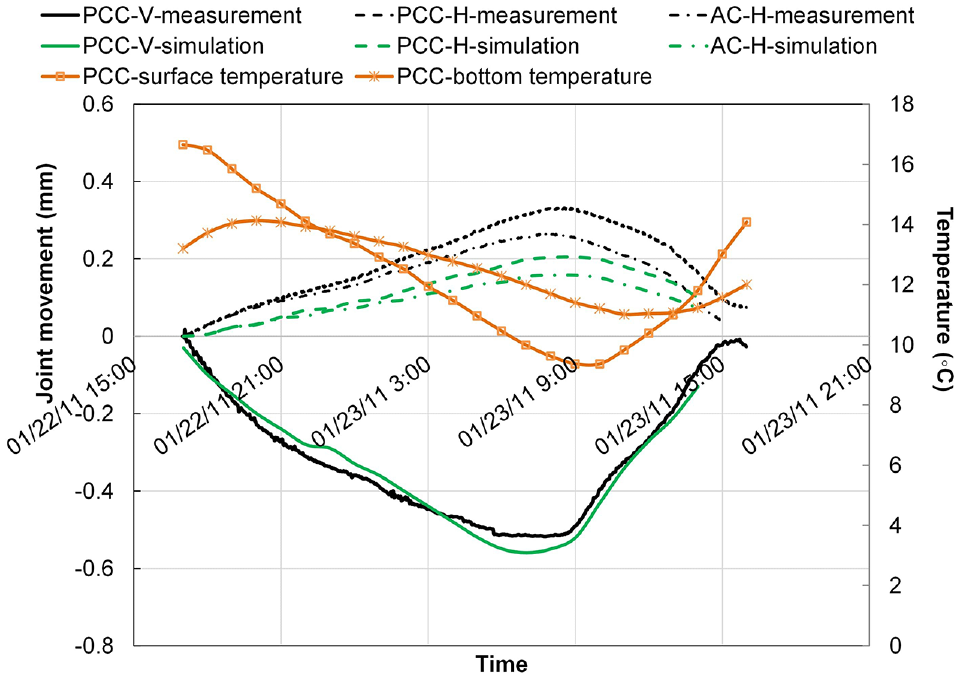
Comparison between measurement and simulation of joint movements for LaneB-J5.

It can also be seen that where there is good agreement between the simulated and measured vertical joint movements in the PCC slabs with a relative error of below 10%, there are relatively large differences between the simulated and measured horizontal movements at both the PCC and AC layers. The simulated horizontal joint movements were found to be 40% lower than the HVS measurements. It is believed that this large difference can be at least partly attributed to the fully bonded condition assumed between the AC overlay and PCC slabs in the FE model. There may have been some debonding occurred between the two layers in the HVS section. A fully bonded condition is likely to lead to fewer horizontal joint movements than partially debonded conditions. A comparison study among different bonding conditions including fully bonded, partially bonded (some part is tie, and some part is friction), and fully friction between surfaces, has been performed. The simulated horizonal joint movements were larger when the contact is fully friction or partially bonded compared with the fully bonded condition. However, the stress and strain at the bottom of the AC overlay were the largest when the contact condition was set to be fully bonded. Therefore, the fully bonded condition was used in this study as the most critical situation.

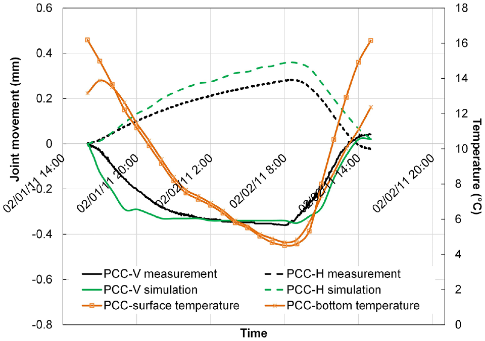
In addition to Lane B, the validation has also been conducted based on Lane C including the horizontal joint movement between PCC slabs and the vertical joint movement of the PCC slab corner. The comparison between simulation results and measurements of joint movements is shown in Figure 9 with the corresponding temperature profile at the PCC surface and PCC bottom. The comparison demonstrates that the simulation result of the vertical movement matches closely with the actual measurement values, whereas the simulated horizontal joint movement of the PCC slabs shows a higher value than the measurement data.

Figure 9.

Comparison results for Lane C-J5 between measurements and simulation of joint movements.

The simulation results and measurement data present an overall acceptable agreement concerning the vertical movement, with relative errors below 10% for Lane B and approximately 20% in the case of Lane C. Conversely, the simulated horizontal joint opening in the PCC slabs shows a greater difference from the measured data with relative errors higher than 40% for Lane B and approximately 30% for Lane C. Meanwhile, Figures 8 and 9 show that the simulated horizontal joint opening is smaller than the measurement for Lane B, whereas the simulation result is larger than the measured data in the case of Lane C, which may be caused by variabilities existing in the two pavement structures and construction in the field.”

Despite the large relative errors in the prediction of horizontal joint movements, the simulation results show a similar response to the temperature variation as the measurement. In summary, the validation results show that the 3D FE model developed can give reasonably good predictions of the response of composite pavements to thermal loading, with the understanding that bonding condition of the overlay to the slab in the areas near the joints may vary and the model is an extreme case of full bonding.

Simulation Results and Analysis

The results and analysis of the simulations conducted using the validated FE model are presented in this section. It includes pavement responses caused by thermal variations throughout a whole year.

Temperature Profile

Temperatures in the PCC slabs were obtained directly from the thermocouple measurement results. As there were no temperature data collected from the AC overlay for most of the year, the temperatures in the AC overlay, by contrast, were estimated through the Enhanced Integrated Climatic Model (EICM) program based on the climate information and pavement structure. The summarized monthly temperature variations in 2011 are given in Figure 10. The highest temperature in the AC overlay took place in July and the lowest temperature was found in January. With the lowest temperature above zero, it is expected that one-time fracture cracking caused by low temperatures is less likely to occur to this pavement section.

Figure 10.

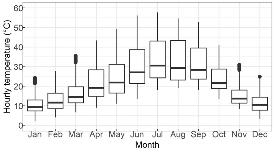
Temperature variations at asphalt concrete (AC) overlay surface in 2011 from Enhanced Integrated Climatic Model (EICM) modeling.

To increase the computational efficiency and reduce the complexity of simulation cases, the temperature profiles in the full year of 2011 in Davis, California were divided into several groups, and only the temperature profile of a single day from each group was assigned to FE model to represent the whole group. A data clustering technique was implemented to achieve this grouping goal. Data clustering is a machine learning technique aiming to partition and segment data. Observations that are grouped together are supposed to have high similarity to each other and low similarity with observations outside the group. The most popular way of clustering is the K-means clustering which divides observations into discrete groups based on some distance metric to minimize the within group point scatter of a dataset. The optimal clustering result is the minimized sum of within-cluster distances to centroids ( 22 ) and the minimum of Equation 8 at a specific K is denoted as $W_{K}$ :

W_{K} (S, C) = \sum_{k = 1}^{K} \sum_{i \in S_{k}} d (i, c_{k})

(8)

where

d = distance measure, typically the squared Euclidean distance or Manhattan distance, and

S = partition produced with K clusters {S₁, S₂… S_K}, each cluster with a centroid C_k (k=1, 2… K).

Two variables were selected for the determination of clustering: the lowest hourly temperature at the AC surface; and the fastest hourly temperature change at the AC/PCC interface ( $Δ T_{h, fast}$ ) which is calculated as Equation 9:

Δ T_{h, fast} = \frac{Highest temperature - Lowest temperature}{Hours between highest and lowest temperature}

(9)

The lowest temperature at the asphalt surface will lead to the highest stiffness of asphalt material which is more critical for the asphalt cracking development, whereas the fastest hourly temperature change at the AC/PCC interface will contribute to the largest PCC contraction deformation as well as the curling deformation.

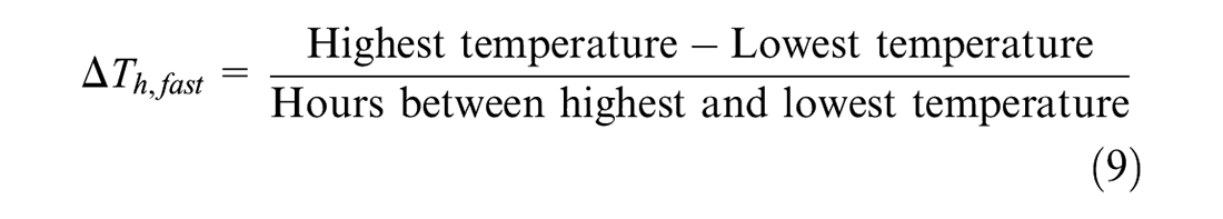
For the K-means method, an appropriate number of clusters needs to be specified first. Choosing the right number of clusters is important in getting a good partitioning of the data. In this study, the number of clusters was determined by the within group sum of squares (WSS) of the two temperature variables, and the “elbow method” was implemented which plots the WSS against the number of clusters (K). The location of the bend (elbow) from the WSS versus K curve is generally considered as an indicator of appropriate number of clustering. The cluster number K and the corresponding WSS value is shown in Figure 11. The elbow plot suggests that five can be the optimal cluster number as it appears to be the bend of the elbow.

Figure 11.

Elbow plot between number of clusters and within group sum of squares (WSS).

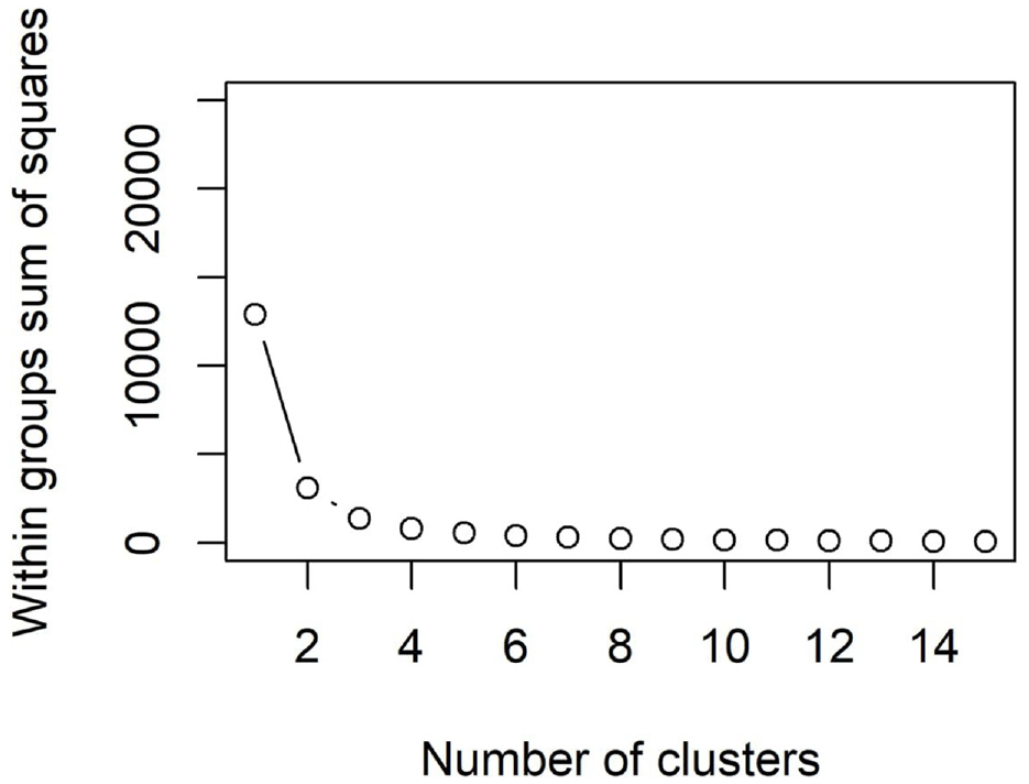
A statistical summary of the two temperature variables is presented as boxplots in Figure 12, a and b . These clustering results depict distinct temperature features among the five groups, especially the lowest temperature at the AC surface. Cluster 5 is the biggest group with 88 data points accounting for 24% of days in 2011, followed by cluster 1 with 86 days. The sizes of clusters 2, 3, and 4 are similar to each other.

Figure 12.

Boxplots of temperature variables distribution for five clusters: (a) cluster summary of the fastest hourly temperature change at the asphalt concrete (AC)/Portland cement concrete (PCC) interface and (b) cluster summary of the lowest temperature at the AC surface.

The highest mean value of the lowest hourly temperature (21.79°C) and the highest mean absolute value of the fastest hourly temperature change (0.77°C/h) were both found in cluster 5. The distribution characteristics for the fastest hourly temperature change for the clusters 1, 2, 3, and 4 do not show significant difference between each other as indicated by the overlapping boxes. By contrast, the boxplots for the lowest hourly temperature variable indicate that the five clusters are significantly different from each other. The combination of the highest temperature and the fastest hourly temperature change makes cluster 5 susceptible to larger thermal strain values in the asphalt overlay caused by the contraction of the underlying PCC slabs and relatively low stiffness of asphalt at high temperatures. Meanwhile, the lowest temperature in cluster 3 would potentially lead to a higher thermal tensile stress in the AC overlay.

Based on the clustering results, the data point closest to the center of each cluster was located through minimizing the Euclidean distance of two temperature variables between the selected center point and the rest. These identified center points and corresponding dates are highlighted in Figure 13. The temperature profile of each day selected is shown in Figure 14. Only temperatures during the time period from 3:00 p.m. to 7:00 a.m. of the next day are displayed in the graph as the highest temperature of the day was commonly observed to occur at 3:00 p.m. and the lowest temperature happened at 7:00 a.m., except for October 7 which was from 11:00 a.m. to 7:00 a.m. Modeling this period of time instead of a whole day not only saved computation time but also enabled the simulations to focus on the critical PCC slab contraction movements.

Figure 13.

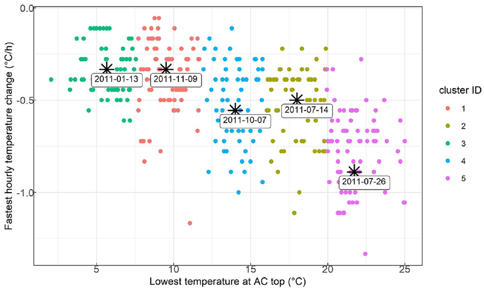
Clustering results with center points and corresponding dates.

Figure 14.

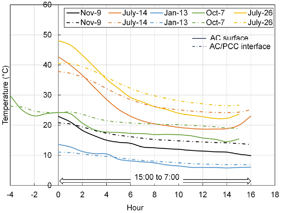
Temperature profiles in pavement (asphalt concrete [AC] surface and interface between AC and Portland cement concrete [PCC]) for the selected five days.

Simulation Result of July 26, 2011

To have a better understanding of the pavement response to daily temperature variations, the 24 h of thermal loading on July 26, 2011 was firstly applied to the 3D FE model before the whole year temperature profiles. The pavement responses including joint movements in the PCC slabs, maximum principal tensile stress (S1) and maximum principal tensile strain (ε1) in the AC overlay were extracted from the simulation results and further examined.

The Cauchy (“true”) stress was obtained from the software ABAQUS, which is directly determined by the traction force and the corresponding acting area. Owing to the viscoelastic behavior of AC material and nonlinear geometric deformation of solid elements in this problem, the maximum principal tensile strain of the logarithmic (“true”) strain (ε1), which is calculated as the log scale of the ratio between final length and initial length, was requested from the simulation output to describe the deformation of asphalt layer under thermal loading. The logarithmic strain (ε1) was selected over engineering strain (ε), which is defined as the ratio of the change in length to its original length, as the logarithmic strain is additive for multiple deformation stages and it can better capture the nonlinear behavior of asphalt material. The relationship between logarithmic strain (ε1) and engineering strain (ε) can be described as: ε1 = ln (1 + ε). This relationship shows that logarithmic strain is always greater than the engineering strain. For example, if the logarithmic strain is 0.1 (100,000 με) then the engineering strain would be 0.105 (105,170 με).

Figure 15 shows the largest movements occurred in the PCC slabs during the 24 h temperature loading, including the maximum vertical deformation (Figure 15a) and maximum horizontal movement (Figure 15b). Two symmetric planes are also illustrated in the plot for better reading of the results. It can be seen that the highest deflection (upward is positive) is found at the corners of the slabs, whereas the lowest deflection is located at the center of the slab. The largest contraction of the PCC slabs is reflected through the opposite horizontal displacement at two ends of one slab with the horizontal movement at the center of the slab being zero. The joint horizontal movement was then obtained by computing the opening gap between two slabs.

Figure 15.

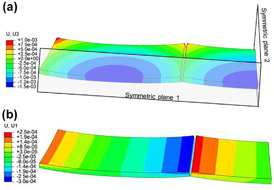
Movement contour in the quarter model of Portland cement concrete (PCC) slabs under thermal loading: (a) vertical deformation (U3) in the PCC slabs and (b) horizontal movement (U1) in the PCC slabs.

Under the thermal loading, PCC slabs were experiencing both curling and contraction–expansion. These deformations cause stress and strain in the AC overlay, especially when the slabs and AC layer are fully bonded. Figure 16 depicts the history of the maximum principal logarithmic strain (ε1) by different colors in the AC overlay at different loading hours (1^st, 5^th, 10^th, 17^th). At the first hour of loading, as there is not much temperature variation in the PCC slabs and asphalt overlay, the whole AC overlay is at an almost-zero strain state. After that, the tensile strain starts to accumulate in the AC overlay right above the joint owing to the hourly temperature drop. The highest strain value occurs around the 15^th hour as shown in Figure 16c. When the temperature climbs up afterwards, the accumulated strain is released as the deformation in the PCC slabs recovers as depicted in Figure 16d. Another interesting observation that can be made from Figure 16 is that except at the area of interest above the joint, the majority of the AC overlay undergoes low values of compressive strain, which makes the area of the AC overlay above joints between PCC slabs more susceptible to cracking.

Figure 16.

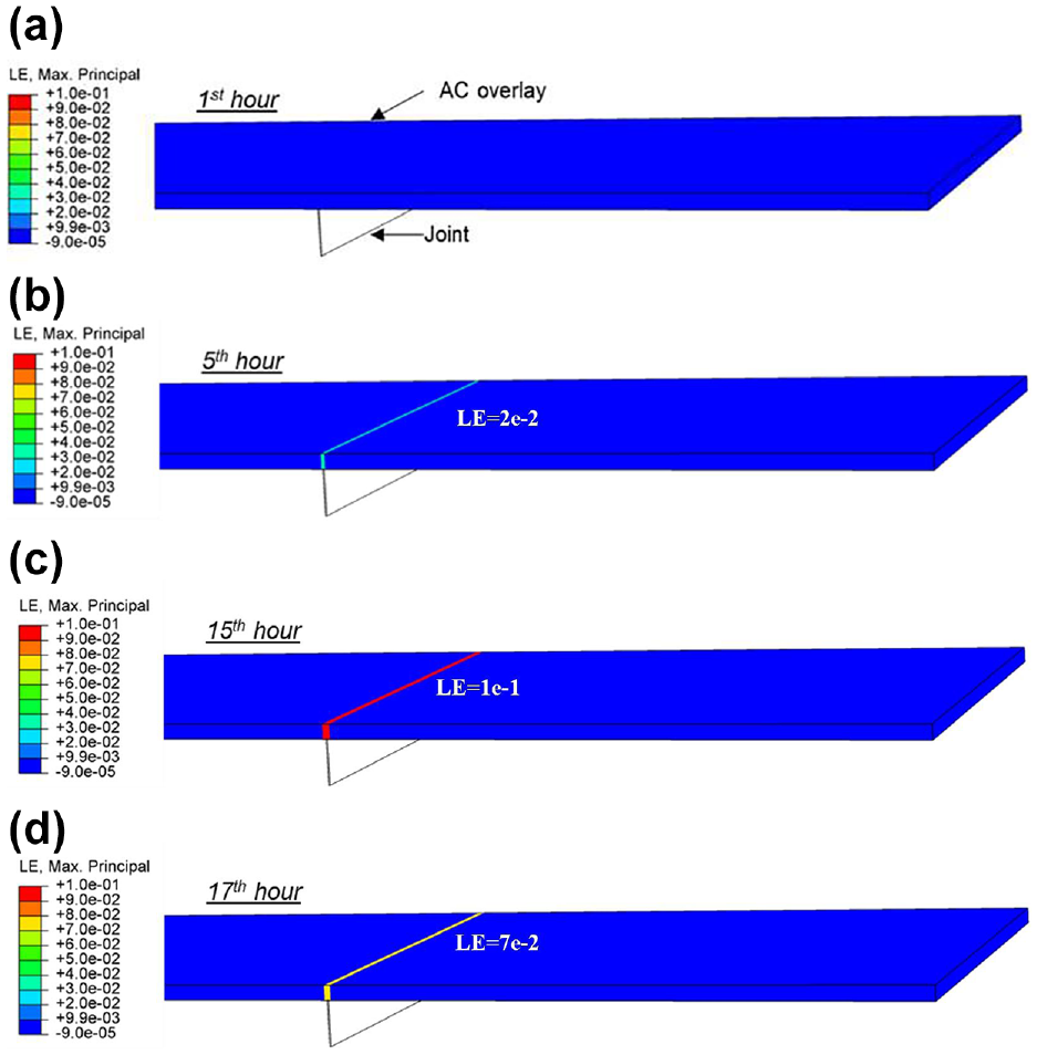
Distribution of maximum principal logarithm strain (LE or ε1) in the asphalt concrete (AC) overlay under thermal loading at: (a) 1^st hour, (b) 5^th hour, (c) 15^th hour, (d) 17^th hour.

The calculated joint movements corresponding to each hour are shown in Figure 17a. They are consistent with expectations for both horizontal and vertical movement versus change of temperature, with the joint horizontal opening and vertical deflection of the slab increasing as the temperature drops and maximums occurring at the coldest hour.

Figure 17.

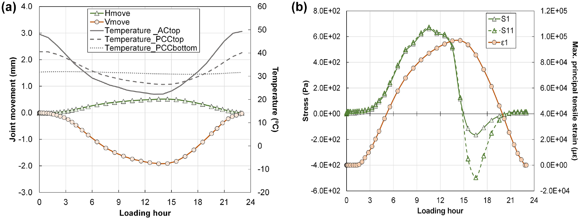
Pavement responses under 24 hours temperature loading: (a) temperature profile in pavement along time and simulated joint movements of the Portland cement concrete (PCC) slabs versus loading hour and (b) simulated maximum principal tensile stress and logarithmic strain versus loading hour.

Figure 17b depicts the hourly evolution of maximum principal tensile stress (S1) and maximum principal logarithmic strain (ε1) in the AC overlay under temperature variation. It can be seen that the AC overlay experiences tensile stress (positive) during the temperature drop and then shifts to compression (negative) after the temperature reaches the lowest point. S1 has also been found to be controlled by the normal tensile stress (S11) in the traffic direction as a consequence of the PCC joint opening. At the 15^th hour, both S1 and S11 become compressive (negative) which could come from the compressive thermal stress in the AC overlay: when the temperature in the overlay reaches the lowest value at the 15^th hour and starts to increase, the asphalt material is experiencing thermal expansion under constraints from the fully bonded PCC layer. In addition, the upward curling deformation of PCC slabs leads to the position of maximum tensile stress occurring at the surface of the AC overlay. The maximum principal strain shows a comparable pattern with the temperature change: ε1 increases as the temperature decreases, and the logarithmic strain reaches a peak when the pavement is experiencing the lowest temperature. The highest tensile stress caused by the temperature drop from 50°C to 20°C at the AC surface is approximate 670 Pa, whereas a rather larger thermal strain value of 100,000 µε has been obtained from the simulation results.

Pavement Responses for Different Clusters

The temperature profiles from the five distinctive clusters shown in Figure 14 were applied to the 3D FE model. The pavement responses from each temperature cluster including horizontal joint opening, vertical movement of slab corner, and maximum principal tensile strain, are shown from Figure 18, plotted against the loading hour. As explained in the previous section, the 0 h represents the highest temperature of a day (except for October 7 when the highest temperature occurs 4 hours earlier) and at the 15^th hour or 16^th hour, the temperature is lowest. Figure 18a displays a clear trend of both horizontal joint opening and vertical deflection of slab corner (absolute value of corner vertical movement) increasing with time. Among these five clusters, January 13 has the lowest daily temperature and the smallest hourly temperature change. Therefore, the joint movement on January 13 is the smallest among the five clusters. Conversely, the temperature profile on July 26 indicates a higher daily temperature as well as a larger value of the fastest hourly temperature change, which matches well with the biggest joint movements observed in Figure 18a. The simulated horizontal joint movement of 0.5 mm on July 26 for a temperature change of 15°C in pavement agrees with a previous research study ( 23 ).

Figure 18.

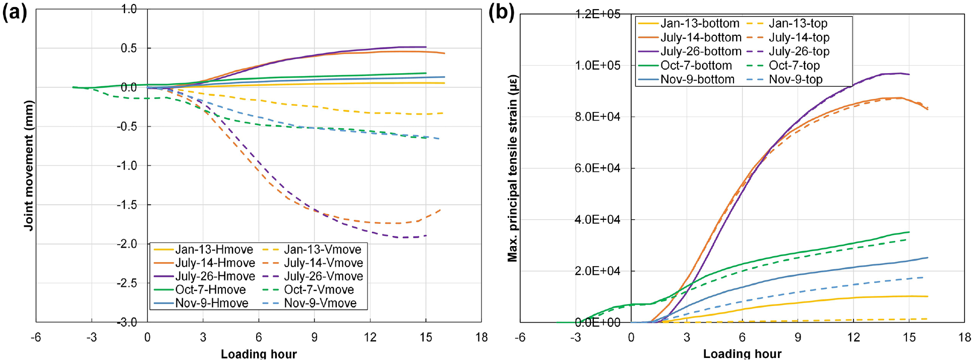
Pavement responses from finite element (FE) model simulation for five temperature clusters: (a) joint movements versus loading hour for the five temperature clusters and (b) maximum principal tensile strain versus loading hour for the five clusters.

Tensile strains at two locations in the AC overlay have been obtained: top and bottom of the AC overlay right above the center of the joints. Comparable principal tensile strains have been noticed in Figure 18b at the bottom and top of the asphalt layer. With the temperature increases from 0-h (−4 h for October 7) to the 15-h, the tensile strains of the five clusters increase as well. July 26 shows the largest strain value potentially owing to the viscous deformation of asphalt material at such a high temperature. By contrast, the low temperature on January 13 causes the asphalt material to respond with more elastic behavior with greater stiffness. Therefore, the lowest tensile strain is expected on January 13 as shown in Figure 18b.

For better comparison among the five clusters, a summary of pavement responses for each temperature cluster is presented in Figure 19. The biggest values of maximum principal tensile stress and maximum principal tensile strain are provided for each cluster regardless of the location being on top of the asphalt overlay or bottom. In future development of this analysis approach, differences in aging between the top and bottom of the overlay will be considered. For the five clusters, the maximum principal tensile stress displays an opposite trend with the maximum principal tensile strain. Particularly, the highest maximum principal tensile strain value and the lowest maximum principal tensile stress occur on July 26, whereas the lowest maximum principal tensile strain value and the highest maximum principal tensile stress are found in the simulation results from January 13. Across the whole simulation year of 2011, the maximum principal tensile strain for five clusters ranges from 10,000 µε to 100,000 µε. As for the tensile stress, the value of maximum principal tensile stress varies from 600 Pa to 15,000 Pa.

Figure 19.

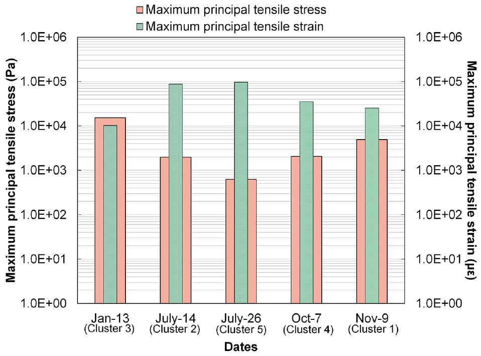
Pavement response summary for the five clusters.

Owing to the limited thermal strain and stress measurements from the test tracks, the FE model was validated mainly against the global responses (joint movements). To make up this limitation, a laboratory test was performed on an asphalt mixture beam by hanging the beam with a static weight attached to the end of the beam to induce a tensile stress of 20,000 Pa similar to the thermal stress on January 13 (cluster 3). After hanging the asphalt mixture beam for 13 h, the measured strain was approximately 6,000 με which is close to the simulated thermal strain from the FE model.

To evaluate the potential of single-event fracture cracking in the AC overlay under such a thermal loading, the tensile stress was compared against the strength of the asphalt material. The strength of the asphalt material is related to the loading rate and temperature. Normally, a faster loading rate or lower temperature will lead to a higher strength value ( 24 – 26 ). The relationship was built between the strength and strain rate at the temperature of 10°C for an asphalt mixture with a maximum nominal aggregate size of 22 mm and a polymer modified binder ( 27 ), as shown in the following Equation 10:

tensile strength (MPa) = 0.1305 \times \ln (strain rate [μ ε / s]) + 0.456

(10)

For the thermal loading on January 13, the hourly temperature fluctuated around 10°C. The strain rate could be calculated as the average rate within the total applied time (16 h for January 13), which would be $10, 000 μ ε / (16 \times 3, 600 s) = 0.174 μ ε / s$ . As a result, the tensile strength based on Equation 10 was estimated to be 0.76 MPa. The ratio between the tensile strength (0.76 MPa) and the maximum tensile stress (15 kPa or 0.015 MPa) on January 13 was approximately 51, indicating that the tensile stress caused by moderate temperature variation is much lower than the strength of asphalt mixtures and under this circumstance, the AC overlay is unlikely to experience one-time fracture cracking. Instead, the asphalt overlay will be subjected to repeated thermal loading with a relatively larger strain value compared with traffic-induced strain value. Such a higher tensile strain value may lead to thermal reflective cracking occurring before traffic-related reflective cracking especially when the AC overlay and the underlying layer is fully bonded but depending on the amount of heavy truck traffic. The thermal strains will occur 365 times per year, whereas the traffic strains will occur more frequently in the truck lanes and less frequently in the lanes that trucks do not use.

Summary and Conclusion

This study investigated the pavement responses that are likely to affect thermal reflective cracking by running 3D FE simulations of AC overlays over PCC slabs under moderate daily temperature variations. The model was validated with data from a full-scale test section. The joint movements in the test section were predicted by applying the measured temperature history at multiple depths. The predicted joint movements match the measurement very well in the vertical direction and reasonably well in the horizontal direction. The FE model was then used to estimate critical pavement responses such as maximum stress and strain caused by daily temperature variations throughout a one-year period. A clustering method was used to reduce the 365 days into five clusters. This significantly improved the computational efficiency. The following are the findings from this study:

During a temperature cycle of 24 h, the pavement structure experiences a temperature decrease and then increase to the next day’s highest temperature. Therefore, the PCC slabs undergo contraction and upward curling at the joints then expansion and downward curling. The area in the AC overlay right above the joint between the PCC slabs is subjected to tensile stress and strain owing to the contraction in the PCC slabs and bending caused by the curling. After reaching the lowest temperature, the tensile stress in the AC overlay turns into compression owing to the downward curling and the expansion of asphalt mixtures, while the tensile strain starts to recover.

In the composite pavement structure studied, the largest tensile stress was estimated to be 10 kPa which occurred on the coldest day, whereas the lowest tensile stress of 0.6 kPa took place on the day with the highest temperature. Conversely, the critical tensile strain is always located above the joint with a neglectable difference in value between the surface and bottom of the asphalt overlay. The highest tensile strain value of 100,000 με happened on the hottest day and the lowest tensile strain on the coldest day was approximately 10,000 με.

The moderate daily temperature variations studied in this study led to relatively high strain values in the AC overlay and relatively low tensile stress compared with the predicted strength, at least for the material used in the simulations which was polymer modified (therefore softer than conventional mixes at intermediate temperatures) and had not experienced long-term aging. These high strains make the pavement susceptible to fatigue damage owing to repetitive thermal loading. Compared with trafficked induced strain, thermal tensile strain is much higher in amplitude but much lower in occurring frequency. Whether thermal loading or traffic loading is more critical for reflective cracking will depend on the amount of truck traffic in the lane.

This study only investigated one climate region and one pavement structure. In addition, the FE model was mainly validated based on global responses measured from the field. Therefore, limited conclusions were presented. However, this study method and framework could be implemented for other climate regions with similar moderate temperature profile and various pavement structures. These findings also provide good bases for the experimental design of a laboratory testing program needed to develop thermal fatigue damage models for thermal loading (large strain/slow loading conditions) similar to the damage models developed for traffic loading induced strain values. These thermal fatigue damage models can then be used to incorporate the impact of moderate daily temperature variations in ME design.

Footnotes

Author Contributions

The authors confirm contribution to the paper as follows: study conception and design: LJ, JH, RW; data collection: LJ, RW, HD; analysis and interpretation of results: LJ, RW, JH; draft manuscript preparation: LJ, JH, RW, HD. All authors reviewed the results and approved the final version of the manuscript.

Declaration of Conflicting Interests

This paper presents research work that was sponsored by the California Department of Transportation (Caltrans). This sponsorship and interest are gratefully acknowledged. The opinions and conclusions expressed in this paper are those of the authors and do not necessarily represent those of the State of California or the Federal Highway Administration.

Funding

The authors received no financial support for the research, authorship, and/or publication of this article.

ORCID iDs

Liya Jiao

Rongzong Wu

References

Harvey

Chong

Roesler

Climate Regions for Mechanistic—Empirical Pavement Design in California and Expected Effects on Performance. University of California-Berkeley, Pavement Research Center, Richmond, 2000.

Dave

E. V.

Song

S. H.

Buttlar

W. G.

Paulino

G. H.

Reflective and Thermal Cracking Modeling of Asphalt Concrete Overlays. Advanced Testing and Characterization of Bituminous Materials, Vol. 2, 2007, pp. 1241–1252.

Dave

E. V.

Buttlar

W. G.

Leon

S. E.

Behnia

Paulino

G. H.

IlliTC-Low-Temperature Cracking Model for Asphalt Pavements. Road Materials and Pavement Design, Vol. 14, 2013, pp. 57–78. https://doi.org/10.1080/14680629.2013.812838.

Gonzalez-Torre

Calzada-Perez

M. A.

Vega-Zamanillo

Castro-Fresno

Evaluation of Reflective Cracking in Pavements Using a New Procedure That Combine Loads with Different Frequencies. Construction and Building Materials, Vol. 75, 2015, pp. 368–374. https://doi.org/10.1016/J.CONBUILDMAT.2014.11.030.

Carpenter

S. H.

Lytton

R. L.

Epps

J. A.

Environmental Factors Relevant to Pavement Cracking in West Texas. Publication TTI-2-8-73-18-1 Intrm Rpt. Texas Transportation Institute, Texas A & M University, College Station, 1974.

Al-Qadi

I. L.

Hassan

M. M.

Elseifi

M. A.

Field and Theoretical Evaluation of Thermal Fatigue Cracking in Flexible Pavements. Transportation Research Record: Journal of the Transportation Research Board, 2005. 1919: 87–95.

Epps

Thermal Behavior of Crumb-Rubber Modified Asphalt Concrete Mixtures. University of California, Berkeley, 1997.

Finn

Saraf

Kulkarni

Nair

Smith

Abdullah

The Use of Distress Prediction Subsystems for the Design of Pavement Structures. Proc., 4th International Conference on Structural Design of Asphalt Pavements, Ann Arbor, MI, University of Michigan, 1977, pp. 3–38.

Hossain

Azam

Mehta

Shaik

Islam

M. R.

Tarefder

Determining and Validating Thermal Strain in Asphalt Concrete. Procedia Engineering, Vol. 145, 2016, pp. 1036–1043. https://doi.org/10.1016/j.proeng.2016.04.134.

10.

Lytton

R. L.

Tsai

F.-L.

Lee

S. I.

Luo

Zhou

NCHRP 669: Models for Predicting Reflection Cracking of Hot-Mix Asphalt Overlays. National Academies Press, Washington, D.C., 2010. https://doi.org/10.17226/14410.

11.

Rao

Darter

Tompkins

Vancura

Khazanovich

Signore

Coleri

Harvey

Vandenbossche

Composite Pavement Systems, Volume 1: HMA/PCC Composite Pavements. Transportation Research Board, Washington, D.C., 2013. https://doi.org/10.17226/22685.

12.

R. Z.

Harvey

J. T.

Evaluation of Reflective Cracking Performance of Asphalt Mixes with Asphalt Rubber Binder Using HVS Tests and Non-Local Continuum Damage Mechanics. Proc., 6th International RILEM Conference on Cracking in Pavements, Chicago, IL, CRC Press/Balkema, The Netherlands, 2008, pp. 3–12.

13.

Baek

Al-Qadi

Reflective Cracking: Modeling Fracture Behavior of Hot-Mix Asphalt Overlays with Interlayer Systems. Journal of the Association of Asphalt Paving Technologists, Vol. 78, 2009, pp. 673–638.

14.

Pais

J. C.

Pereira

P. A. A.

Predictions of Existing Reflective Cracking Potential of Flexible Pavements. Proc., 4th International RILEM Conference, Ontario, RILEM Publications S.A.R.L, Cachan, France, 2000, pp. 155–164.

15.

Dave

E. V.

Leon

Park

Thermal Cracking Prediction Model and Software for Asphalt Pavements. Proc., First Congress of Transportation and Development, ASCE, Reston, VA, 2011, pp. 667–676.

16.

Han

Sha

Jiao

Modeling to Simulate Inverted Asphalt Pavement Testing: An Emphasis on Cracks in the Semirigid Subbase. Construction and Building Materials, Vol. 306, 2021, p. 124790. https://doi.org/10.1016/j.conbuildmat.2021.124790.

17.

Jiao

Harvey

Reflective Crack Initiation of Asphalt Overlays on Jointed Concrete Pavement Using Finite Element Model. International Journal of Pavement Engineering, 2022, pp. 1–15. https://doi.org/10.1080/10298436.2022.2154350

18.

Choi

J. W.

Harvey

J. T.

Extended Kalman Filter and Its Application in Pavement Engineering. Studies in Computational Intelligence, Vol. 259, 2009, pp. 239–253. https://doi.org/10.1007/978-3-642-04586-8_8.

19.

Hussein

H. M. E.

Halim

A. A. E.

Differential Thermal Expansion and Contraction: A Mechanistic Approach to Adhesion in Asphalt Concrete. Canadian Journal of Civil Engineering, Vol. 20, 1993, pp. 366–373. https://doi.org/10.1139/l93-051.

20.

Davids

Turkiyyah

Mahoney

EverFE—Rigid Pavement Three-Dimensional Finite Element Analysis Tool. Transportation Research Record: Journal of the Transportation Research Board, 1998. 1629: 41–49.

21.

Huang

Y. H.

Pavement Analysis and Design. Pearson Prentice Hall, Upper Saddle River, NJ, 2004.

22.

Chiang

M. M. T.

Mirkin

Intelligent Choice of the Number of Clusters in K-Means Clustering: An Experimental Study with Different Cluster Spreads. Journal of Classification, Vol. 27, 2010, pp. 3–40. https://doi.org/10.1007/s00357-010-9049-5.

23.

Akentuna

Kim

S. S.

Nazzal

Abbas

A. R.

Asphalt Mixture CTE Measurement and the Determination of Factors Affecting CTE. Journal of Materials in Civil Engineering, Vol. 29, 2017, p. 04017010. https://doi.org/10.1061/(asce)mt.1943-5533.0001840.

24.

Teltayev

Radovskiy

Predicting Thermal Cracking of Asphalt Pavements from Bitumen and Mix Properties. Road Materials and Pavement Design, Vol. 19, 2018, pp. 1832–1847. https://doi.org/10.1080/14680629.2017.1350598.

25.

Peng

Yuan

Zhu

Liu

Investigation on Strength Characteristics of Bio-Asphalt Mixtures Based on the Time–Temperature Equivalence Principle. Construction and Building Materials, Vol. 309, 2021, p. 125132. https://doi.org/10.1016/J.CONBUILDMAT.2021.125132.

26.

Espinosa

Caro

Wills

Study of the Influence of the Loading Rate on the Fracture Behaviour of Asphalt Mixtures and Asphalt Mortars. Construction and Building Materials, Vol. 262, 2020, p. 120037. https://doi.org/10.1016/J.CONBUILDMAT.2020.120037.

27.

Steiner

Hofko

Dimitrov

Blab

Impact of Loading Rate and Temperature on Tensile Strength of Asphalt Mixtures at Low Temperatures. Proc., 8th RILEM International Conference on Mechanisms of Cracking and Debonding in Pavements, Springer, Dordrecht, Netherlands, 2016, pp. 69–74. https://doi.org/10.1007/978-94-024-0867-6_10.

Study on Thermal Reflective Cracking of Asphalt Concrete Overlays on Concrete Pavements Under Moderate Temperature Variations Using Finite Element Model

Abstract

Keywords

FE Model for Thermal Loading

FE Model Information

Model Geometry and Boundary Condition

Material Property

Loading

Mesh Convergence

FE Model Validation

Simulation Results and Analysis

Temperature Profile

Simulation Result of July 26, 2011

Pavement Responses for Different Clusters

Summary and Conclusion

Footnotes

Author Contributions

Declaration of Conflicting Interests

Funding

ORCID iDs

References