Sage Journals: Discover world-class research

Abstract

Impact echo (IE) is capable of locating subsurface defects in concrete slabs from the vibrational response of the slab to a mechanical impact. For an intact slab (“good” condition), the frequency spectrum of the IE is dominated by a single peak corresponding to the slab’s “thickness resonance frequency,” whereas the presence of subsurface defects (“fair” or “poor” conditions) could manifest in various ways such as multiple distinct peaks at frequencies higher, or lower, than the thickness resonance. In previous research, the authors have proposed a frequency partitioning of the spectrum for IE signal classification. Firstly, the thickness resonance frequency band is identified using a data-driven approach and then the IE signals are represented by their energy distribution in three bands—frequencies less than, within, and greater than the thickness resonance. Following this feature extraction, an unsupervised clustering approach is used to identify the centroids for each signal class—good, fair, and poor—which are further used to classify any test signal into one of the three aforementioned classes. The classification is developed by training on unlabeled IE signals from real bridge deck data (the Federal Highway Administration’s [FHWA’s] InfoBridge dataset) without making use of any labeled data. This study aims to validate the proposed methodology on a labeled dataset of eight reinforced concrete specimens constructed at the FHWA Advanced Sensing Technology Nondestructive Evaluation laboratory having known artificial defects. Our findings indicate that the physics-based feature definition and the method developed on real bridge data are robust and can classify IE signals in the labeled data with moderate accuracy.

Keywords

nondestructive testing impact echo signal classification machine learning physics-based

Condition monitoring and evaluation of bridge decks are imperative to maintaining structural reliability during their service life. Concrete bridge decks are traditionally evaluated using visual inspection methods. Nondestructive evaluation (NDE) techniques have been increasingly popular for the condition evaluation of bridge decks to indicate volumetric damage and deterioration that might not be visible from the surface ( 1 – 7 ). NDE techniques rely on various physical phenomena (acoustic, electric, thermal, etc.) to identify specific indicators of the deterioration processes. For instance, concrete durability assessment with respect to corrosion can be done using electrical resistivity (ER) and half-cell potential (HCP) tests ( 8 , 9 ), while the electromagnetic properties of the material, the location of reinforcement, and the presence of voids can be learned using ground penetrating radar (GPR) ( 10 ). Of particular interest are ultrasonic or acoustic methods, such as impact echo (IE), that can identify and accurately detect the presence of discontinuities such as debonding or delamination within a material ( 11 – 14 ) (say, concrete bridge decks).

IE excites and records the modal frequencies corresponding to the thickness resonance of the slab, geometric boundaries, and crack-like defects running parallel to the surface (delamination) under a mechanical impact. IE responses (or signals) are typically analyzed in the frequency domain (using the fast Fourier transform algorithm) and the spectral responses are interpreted to assess the condition of the test slab and identify potential defects. See Figure 1 for an illustration of the IE signal–spectrum pair corresponding to each condition—good, fair, and poor. The IE spectrum for a slab in “good” condition, that is, free from damage, exhibits a unimodal spectrum with a single-frequency peak corresponding to its thickness resonance frequency ( $f_{h}$ ), since most of the impact energy is reflected from the slab backwall ( 15 ). Similarly, severely deteriorated slabs (“poor” condition) are identified by a dominant low-frequency peak caused by the flexural vibrations of the debonded concrete. However, the frequency associated with these vibrations is considerably lower than the thickness resonance frequency ( $f_{h}$ ). In contrast, moderate damage (“fair” condition) or deep delamination typically introduces additional higher frequency components ( $f_{d}$ greater than $f_{h}$ ) in the spectrum caused by the reflections from the deeper delaminations. Therefore, the distribution of energy across frequencies varies depending on the type and extent of damage, suggesting the appropriateness of spectral analysis for IE signal interpretation. However, Fourier transform-based approaches have known limitations for analyzing non-stationary IE signals. Therefore, a two-dimensional joint time–frequency analysis (say, using wavelet transform) may be used as an alternative for feature extraction.

Figure 1.

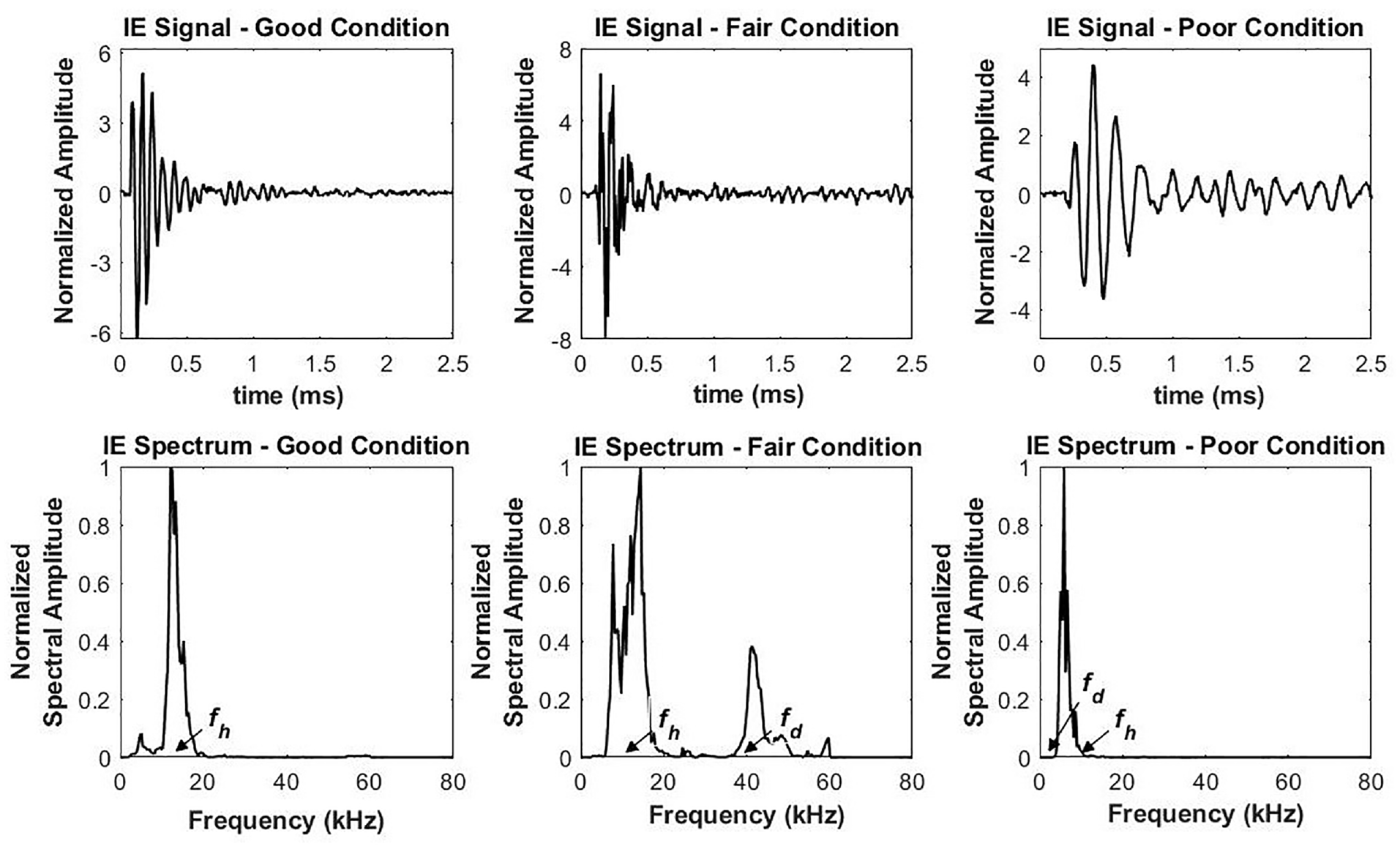
Impact echo (IE) signals and spectra corresponding to three different delamination conditions: good, fair, and poor.

Although effective in detecting damage and delamination in concrete slabs, manual IE data interpretation has limited utility in bridge condition evaluation practices. Moreover, there exists limited research on data-driven approaches to automatically classify IE signals. Prior research on automated IE signal analysis relies on machine learning (ML) algorithms such as the support vector machine ( 16 ) and deep learning (DL) ( 17 – 22 ). However, DL models require large data volumes for their training, which is often not the case for labeled IE signals. Limited availability of labeled IE data could lead to model “overfitting”—a phenomenon where the model fails to generalize its performance to “unseen” data. As demonstrated by Dorafshan and Azari ( 21 ), transfer learning is an efficient way to tackle this problem. Therefore, the limitations of DL and the scarcity of labeled IE data motivate the development of an unsupervised modeling approach, as proposed in previous research ( 23 ). Based on the distinct spectral characteristics of the three conditions (good, fair, and poor) in that study, the authors have partitioned the frequency spectrum into three non-overlapping bands having frequencies less than, within, and greater than the thickness resonance frequency. The energy in each of the bands is used as a feature definition in that study. Subsequently, IE signals are classified into one of the three categories—good, fair, or poor—based on their spectral signatures. This classification scheme was developed using unlabeled IE signals from the Federal Highway Administration’s (FHWA’s) Long Term Bridge Performance (LTBP) InfoBridge dataset. The objective of this study is to validate the classification scheme on a set of experimental slabs with “known” subsurface damages (therefore labeled IE data) from the FHWA Advanced Sensing Technology (FAST) NDE laboratory. Subsurface defect classification for bridge decks using IE from the FAST dataset has also been demonstrated ( 21 , 22 ) using DL models. The remainder of the paper is organized as follows. Firstly, the IE data used are described, followed by the thickness resonance estimation and classification methodology as proposed by Sengupta et al. ( 23 ). Next, we present the validation results on the experimental concrete slabs, followed by a discussion on the robustness of the model.

Data Description

In this study, the results of IE tests performed on eight reinforced concrete slabs at the FAST NDE laboratory are used for validation purposes. Each concrete slab, 3.0 m long, 1.0 m wide, and 0.2 m thick, is constructed with “known” artificial defects—shallow delamination, deep delamination, honeycombing, voids, and a transverse vertical crack, as shown in Figure 2. These defects extend 0.30 m along the length of the specimens and 0.20 m along the width of the specimens. The concrete slabs are constructed by a normal-weight concrete mix with a water-to-cement ratio of 0.37 and have a 28-day compressive strength of 27.6 MPa, with two mats of uncoated steel reinforcements of 15.8 mm diameter at 203 mm spacing in both the lateral and transverse directions. Several NDE techniques including IE are used to understand their efficacy and feasibility in detecting subsurface defects. IE tests are performed at a regular grid on the concrete slabs with a grid spacing of 100 mm, both longitudinally and transversely. The test setup consists of an impact source (11 mm diameter steel spheres on spring rods) and a receiving transducer or sensor (e.g., an accelerometer). IE signals are recorded at a sampling frequency of 200 kHz for a duration of 10 ms at every point of the grid. There are 252 recorded IE signals per laboratory concrete slab. Further details on the construction of concrete slabs and the testing can be found in Lin et al. ( 24 ).

Figure 2.

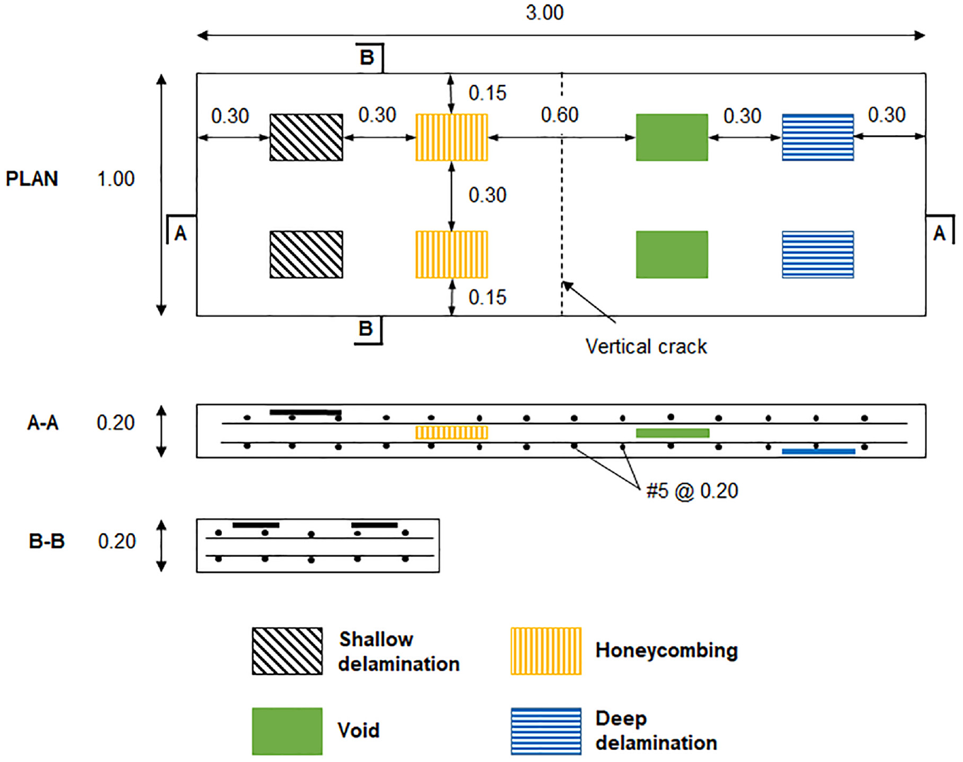
Schematic diagram of the concrete slabs with artificial defects.

Methodology

This section provides a brief summary of the IE signal classification scheme as proposed in previous research ( 23 ).

Estimating the Thickness Resonance Bandwidth

To characterize IE signals, it is necessary to establish the spectral features for “good” signals (recorded at slab locations free from damages), where most of the impact energy is reflected back from the bottom of the deck and the frequency spectrum is dominated by one frequency peak corresponding to its thickness resonance. This allows us to automatically identify the thickness resonance frequency ( $f_{h}$ ) of the slab. Although there exists an analytical expression (Equation 1) to calculate the thickness resonance frequency for a given slab thickness ( $h$ ) and P-wave velocity ( $V_{p}$ ), these parameters might not be readily available as with publicly available databases such as the LTBP InfoBridge:

f_{h} = C \frac{V_{p}}{2 h} where C is 0.94 - 0.96 for concrete slabs

(1)

Therefore, a data-driven approach was developed to estimate the thickness resonance frequency. The IE spectra for all points in the test slab are analyzed to identify the peak frequency corresponding to the maximum energy content in each spectrum. The peak frequency values for all test points on the slab are aggregated to identify the most prevalent frequency peak, which is an indicator of the thickness resonance frequency for each bridge deck. The inherent assumption in this approach is that the thickness resonance is excited at most test points, except at extremely deteriorated points, where the flexural mode of vibration dominates. To estimate the thickness resonance bandwidth, the histogram of peak frequencies is parameterized with a Gaussian mixture model (GMM) assuming that all data points are generated from a mixture of a finite number of Gaussian distributions with unknown parameters. The parameters of the GMM are estimated using an expectation-maximization technique, while the number of Gaussian components in the mixture model is decided based on the Bayesian information criterion (BIC) score. The BIC score provides a weighted measure of the change in the log-likelihood function when different numbers of GMM components are considered. The lowest BIC score provides the model that would be closest to the model with the maximum log-likelihood value, and therefore is chosen as the final model. Once the GMM is fitted with an optimum number of mixture components, the Gaussian distribution with the maximum mixture proportion is chosen as a representation of the thickness resonance. The mode ( $f_{m}$ ) of this distribution and $f_{m} \pm 3 σ$ are used as the point estimate and interval estimate of the thickness resonance frequency of the slab, respectively.

Partitioning the IE Power Spectrum

IE signals corresponding to different conditions (good, fair, and poor) have distinct spectral patterns, that is, the distribution of energy among frequencies differs based on the type and extent of damage. Therefore, the energy content in each frequency band might be an indicator of the damage state represented by the IE signal. Once the thickness resonance band of the deck is estimated, the IE spectrum for each signal is analyzed to calculate the energy in the three non-overlapping bands—frequencies less than (Band 1), within (Band 2), and greater than (Band 3) the thickness resonance frequency. Therefore, each IE signal is represented by a three-dimensional vector of the proportion of energy in each band in order, that is, $[p_{1}, p_{2}, p_{3}]$ , where $p_{i}$ refers to the proportion of energy in the ith band. For example, for a “good” signal, since most of the impact energy is concentrated within the thickness resonance band (i.e., Band 2), it is expected that the energy proportion is shifted toward coordinate $[0, 1, 0]$ in the feature space, while a feature representation of a “poor” signal is skewed toward $[1, 0, 0]$ .

Classification of IE Signals

Each IE signal is represented by a three-dimensional feature vector of energy proportions in the three bands: Bands 1–3. The feature vectors are input to an unsupervised clustering algorithm, that is, $k$ -means ( 25 ) with $k$ = 3. The $k$ -means clustering is performed on the feature vectors from all slabs to partition the feature space into three distinct regions and identify the centroids corresponding to “good,”“fair,” and “poor” signal classes. As a result, each signal in the training dataset is assigned to a particular condition class. The classification of a test (unseen) signal then becomes a supervised learning problem. During the inference phase, a test signal is first transformed into the feature vector and then classified into one of the three classes (good, fair, or poor) using a $k$ -nearest neighbor ( $k$ -NN) algorithm with an Euclidean distance metric. Specifically, we use the centroids of the clusters obtained from the $k$ -means algorithm to perform the nearest neighbor search in the classification. Notably, the performance of the clustering approach depends on the observed representation of points in the feature space. Limited data points in the feature space might adversely affect the clustering results. Here, we aggregated IE signals belonging to different conditions (intact and all defect types) for all eight slabs to have sufficient dispersion in the feature space.

Results and Discussion

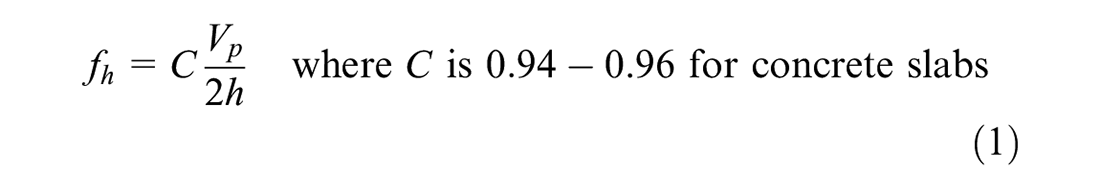
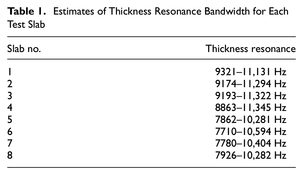
This section details the data analysis and results on the eight concrete slabs. As stated in the Data Description section, the slabs include known built-in artificial defects: shallow and deep delamination, honeycombing, and voids. For each slab, the peak frequency is identified for all IE spectra. Following previous studies on this dataset ( 21 , 22 ), the portion of the IE spectra corresponding to frequencies greater than 20 kHz was discarded as noise. The histograms of the peak frequencies in the IE spectra for each of the eight slabs are shown in Figure 3. We observe that each histogram is characterized by a distinct peak indicating that the majority of the test points on the bridge deck have peak frequencies near 10 kHz. To quantify the thickness resonance bandwidth, Gaussian mixtures are fitted to parameterize the histograms using the BIC score to determine the best number of distributions. Notice that while three Gaussian distributions well characterized the IE spectra for most slabs, for slabs 1, 5, and 8 only two distributions were needed. The Gaussian distribution with the maximum mixture proportion (highlighted in red in the figure) is used for estimating the thickness resonance bandwidths, which are given in Table 1. Using the analytical approach (Equation 1), the thickness resonance frequency is calculated in the range of 8400–10,800 Hz. 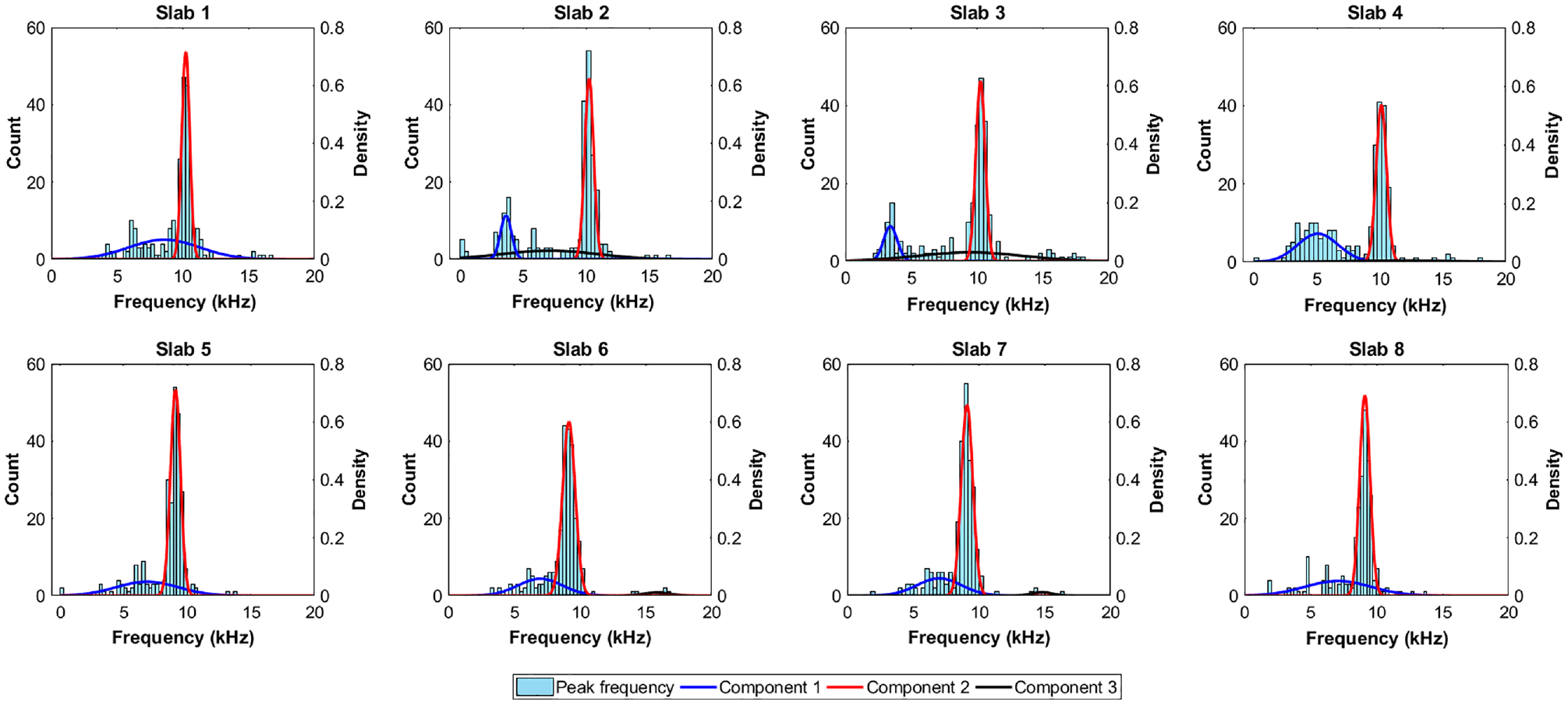These values correspond to P-wave ( $V_{p}$ ) velocities between 3500 and 4500 m/s, using the known slab thickness of $0.2$ m. Therefore, the estimated bandwidths using our proposed data-driven approach are found to be in good agreement with those obtained analytically.

Figure 3.

Histograms of peak frequencies with the fitted Gaussian mixture models for test slabs 1–8 (color online only).

Table 1.

Estimates of Thickness Resonance Bandwidth for Each Test Slab

Slab no.	Thickness resonance
1	9321–11,131 Hz
2	9174–11,294 Hz
3	9193–11,322 Hz
4	8863–11,345 Hz
5	7862–10,281 Hz
6	7710–10,594 Hz
7	7780–10,404 Hz
8	7926–10,282 Hz

Having the thickness resonance bandwidth for each slab, we can now partition the IE spectra into three bands corresponding to lower than, within, and above the thickness resonance band. Next, the proportion of energy in each band is calculated and is used as a $3 \times 1$ feature vector. Note that each value in this feature vector corresponds to the percentage of energy in Bands 1–3. Figure 4 presents the feature space representation of the IE signals belonging to each slab for illustration purposes. Each data point is labeled with the corresponding condition of no defect, shallow delamination, honeycombing, void, and deep delamination. The data points corresponding to shallow delamination and void defects are observed to fall in the lower left-hand side of these figures. This corresponds to IE signals that have the largest energy content in the frequency band less than the thickness resonance, that is, Band 1. Similarly, moderately deteriorated cases (deep delamination and honeycombing) are generally found toward the upper middle part of these figures. This corresponds to having a considerable amount of energy in Band 3 as well, which arises from additional high-frequency components. As expected, spectra corresponding to intact test locations with “no defect” have most energy in the thickness resonance band, that is, Band 2. However, a considerable number of test points labeled as “no defect” have energy concentrations also in Band 3, which could be because some damage occurred during the construction process. Although alternative NDE techniques have not been utilized in this study to identify potential damages in the slabs, research ( 22 , 24 ) on damage identification using IE on the same dataset has highlighted the presence of additional damages in the slabs.

Figure 4.

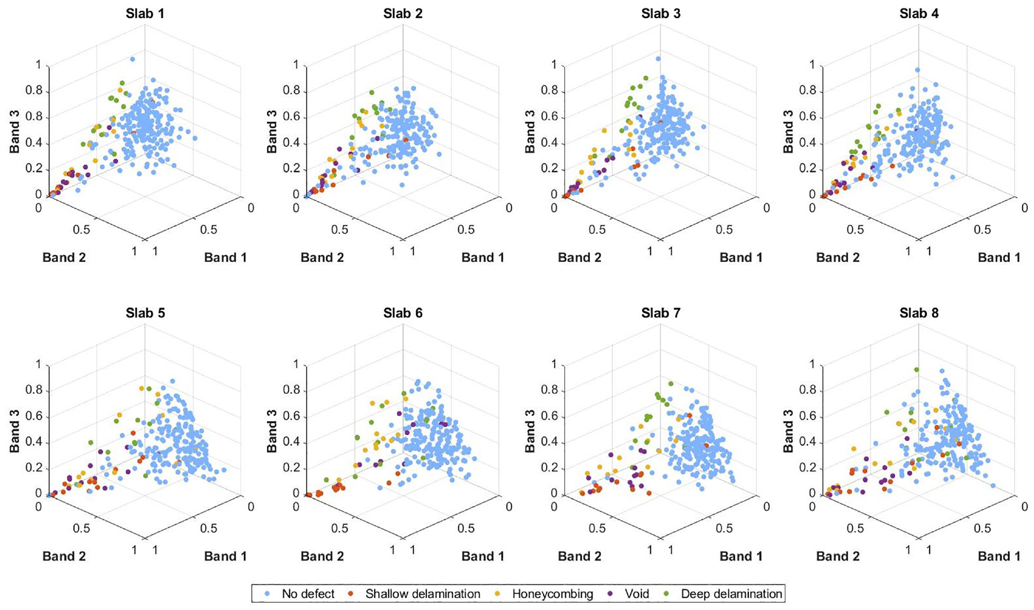
Feature space representations of impact echo signals in test slabs 1–8.

As we observe from Figure 4, except for shallow delamination, IE signals obtained from different damaged portions of the slab are not localized; rather, they show significant scatter in the feature space. This could be because of the limitation of the proposed spectral approach for delamination characterization to distinguish between different damage types. Next, a $k$ -means clustering is performed to identify centroids corresponding to different conditions of the slab. To have sufficiently large number of points in the feature space, a total of 2016 IE signals from all eight slabs are combined and the $k$ -means clustering is performed on the combined dataset to generate three clusters, assumed to correspond to good, fair, and poor conditions, and the centroid of each cluster is identified (see Table 2). To better understand the variance in data across different datasets, the cluster centroids obtained from the experimental data are compared with that obtained from the LTBP dataset (used by Sengupta et al. [ 23 ]), as shown in Table 2. Interestingly, the centroids obtained from the experimental data and LTBP data are in good agreement. Some differences are observed, especially for the signals labeled as “good.” It can be seen that centroids corresponding to “good” signals have higher energy in Band 3 as compared to that obtained from the real bridge data.

Table 2.

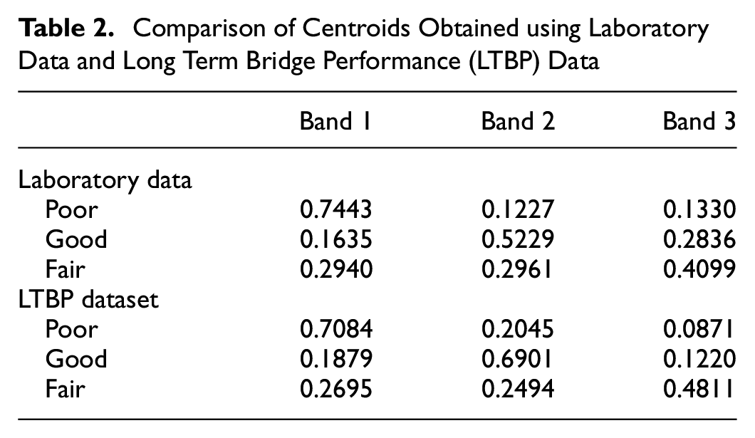
Comparison of Centroids Obtained using Laboratory Data and Long Term Bridge Performance (LTBP) Data

	Band 1	Band 2	Band 3
Laboratory data
Poor	0.7443	0.1227	0.1330
Good	0.1635	0.5229	0.2836
Fair	0.2940	0.2961	0.4099
LTBP dataset
Poor	0.7084	0.2045	0.0871
Good	0.1879	0.6901	0.1220
Fair	0.2695	0.2494	0.4811

Using the centroids of each cluster, each signal in the dataset can be classified into one of three classes—“good,”“fair,” or “poor”—using a $k$ -NN classification (see Figure 5). Further, IE signals corresponding to different defect types in the laboratory slabs may be assigned a label of “good,”“fair,” or “poor,” as shown in Table 3. Notice that the features of the IE signals recorded on portions of the slab with shallow delamination and void defects make up the majority of points labeled as “poor” in Figure 5. This is confirmed in Table 3, which suggests that more than 80% of the IE signals corresponding to shallow delamination or voids fall in the “poor” category. In the cluster labeled “fair,” a mix of IE signal features from portions of the slab with no defects and deep delamination or honeycombing are found. This is again confirmed by Table 3, which shows that the IE signals corresponding to the no defect regions or deep delamination are categorized as “fair” at least 50% of the time. In the “good” cluster, there are mostly IE signal features from the no defect portions of the slab, which is again corroborated in Table 3.

Figure 5.

$k$ -means clustering on the combined dataset.

Table 3.

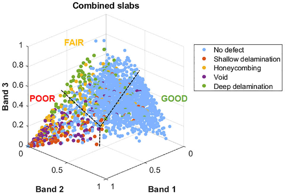
Clustering of Impact Echo Signals from Different Defects

Type of defect ↓	Good	Fair	Poor
Shallow delamination	4	14	82
Honeycomb	4	38	58
Void	3	14	83
Deep delamination	7	69	24
No defect	43	50	7

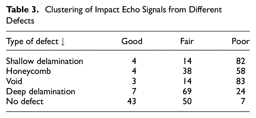
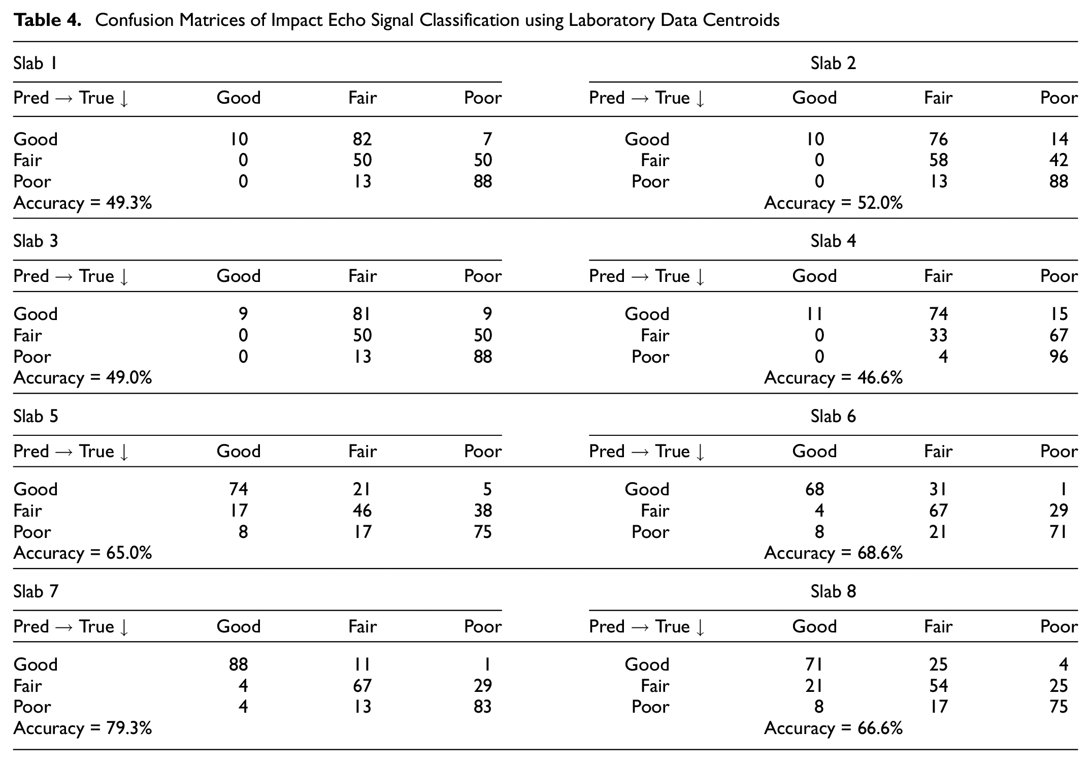
The IE spectra corresponding to voids have significant energy in the frequencies lower than the thickness resonance, which is similar to that of shallow delamination. On the other hand, spectra corresponding to deep delamination and honeycombing have a peak frequency centered around the thickness resonance with additional higher frequency components. Therefore, based on expert opinion (and the clustering results in Table 3), the accuracy of the IE signal classification is evaluated assuming that shallow delamination and voids represent the “poor” condition, deep delamination and honeycombing are the “fair” condition, and no defects are the “good” condition. The classification accuracy based on the centroids identified from the laboratory data is shown in Table 4. Note that in the confusion matrix, the term “True” refers to labels that have been assigned based on expert interpretation. From Table 4 it can be seen that the accuracy of classification for the eight slabs is around 60% on average, ranging from 46% for Slab 4 to 79% for Slab 7. Interestingly, the model performs with a lower accuracy on Slabs 1–4, compared to Slabs 5–8. Regardless, most of the misclassification is caused by a significant number of test points with “no defect” having energy in Band 3 and therefore being classified as in “fair” condition. Figure 6 presents IE signals and their corresponding spectra for two selected locations from Slab 1 that presumably have no defects and two selected locations from Slab 1 that are known to have deep delamination. As can be seen from the figure, spectra corresponding to “no defect” have significant energy in the frequency range greater than 10 kHz, in addition to the peak frequency centered around 10 kHz (thickness resonance). A very similar IE spectra is observed for deep delamination with significant energy in the frequency range greater than 10 kHz, as can be seen in Figure 6. Visual inspection of Figure 6 confirms that some locations with no defects show the signatures of deep delamination in their IE spectra, and the expert classification of these points is “fair.” Therefore, although these locations have no built-in defects, the spectra indicate the possibility of a certain degree of subsurface damage possibly generated during the construction process. Similarly, Dorafshan and Azari ( 22 ) and Lin et al. ( 24 ) have also emphasized the discrepancy in accuracy between the two sets of slabs (Slabs 1–4 versus 5–8), suggesting the presence of subsurface damages in areas without built-in defects.

Table 4.

Confusion Matrices of Impact Echo Signal Classification using Laboratory Data Centroids

Slab 1				Slab 2
Pred → True ↓	Good	Fair	Poor	Pred → True ↓	Good	Fair	Poor
Good	10	82	7	Good	10	76	14
Fair	0	50	50	Fair	0	58	42
Poor	0	13	88	Poor	0	13	88
Accuracy = 49.3%				Accuracy = 52.0%
Slab 3				Slab 4
Pred → True ↓	Good	Fair	Poor	Pred → True ↓	Good	Fair	Poor
Good	9	81	9	Good	11	74	15
Fair	0	50	50	Fair	0	33	67
Poor	0	13	88	Poor	0	4	96
Accuracy = 49.0%				Accuracy = 46.6%
Slab 5				Slab 6
Pred → True ↓	Good	Fair	Poor	Pred → True ↓	Good	Fair	Poor
Good	74	21	5	Good	68	31	1
Fair	17	46	38	Fair	4	67	29
Poor	8	17	75	Poor	8	21	71
Accuracy = 65.0%				Accuracy = 68.6%
Slab 7				Slab 8
Pred → True ↓	Good	Fair	Poor	Pred → True ↓	Good	Fair	Poor
Good	88	11	1	Good	71	25	4
Fair	4	67	29	Fair	21	54	25
Poor	4	13	83	Poor	8	17	75
Accuracy = 79.3%				Accuracy = 66.6%

Figure 6.

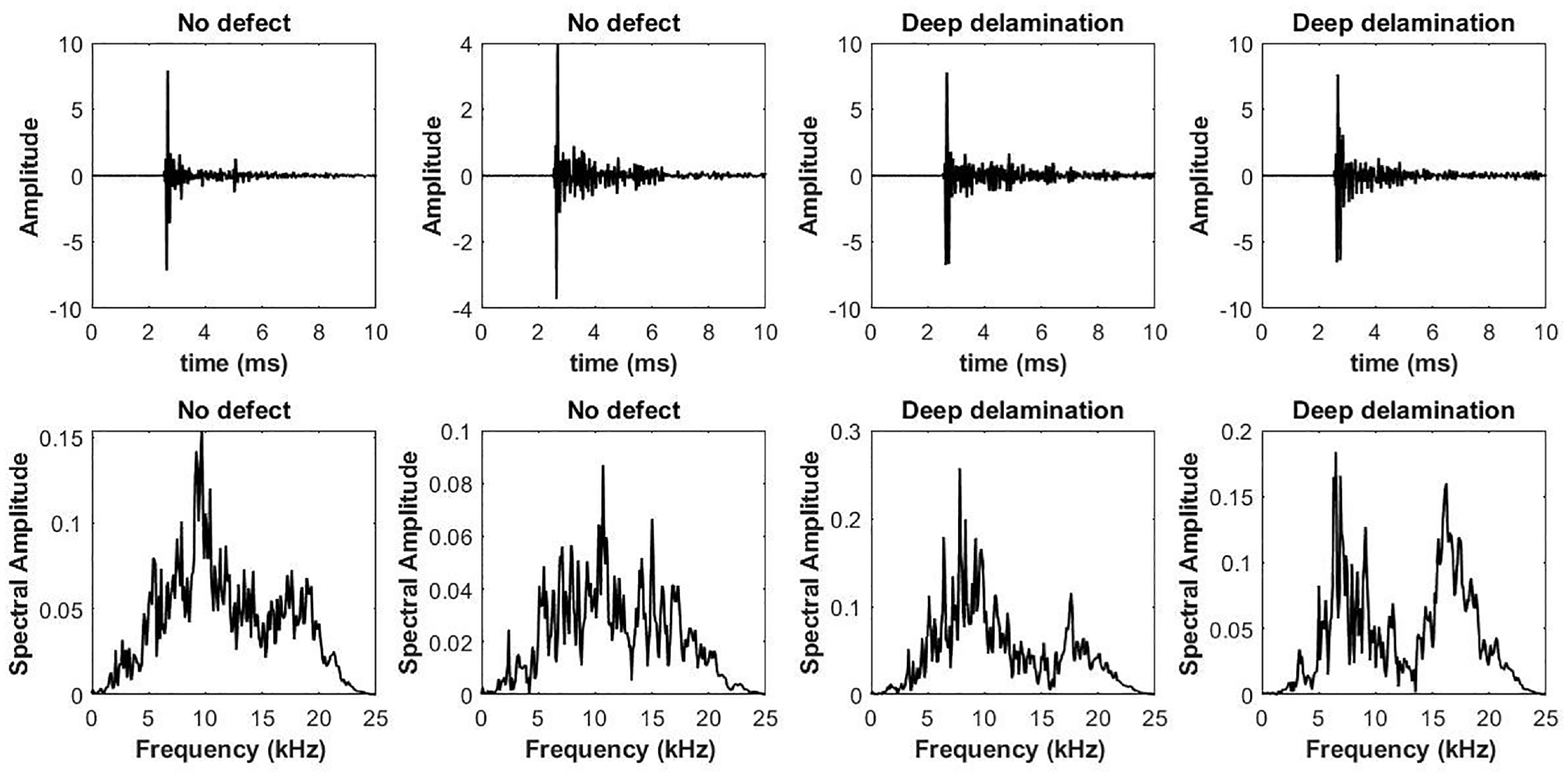
Impact echo signals and spectra for regions with “no defect” and “deep delamination” from Slab 1.

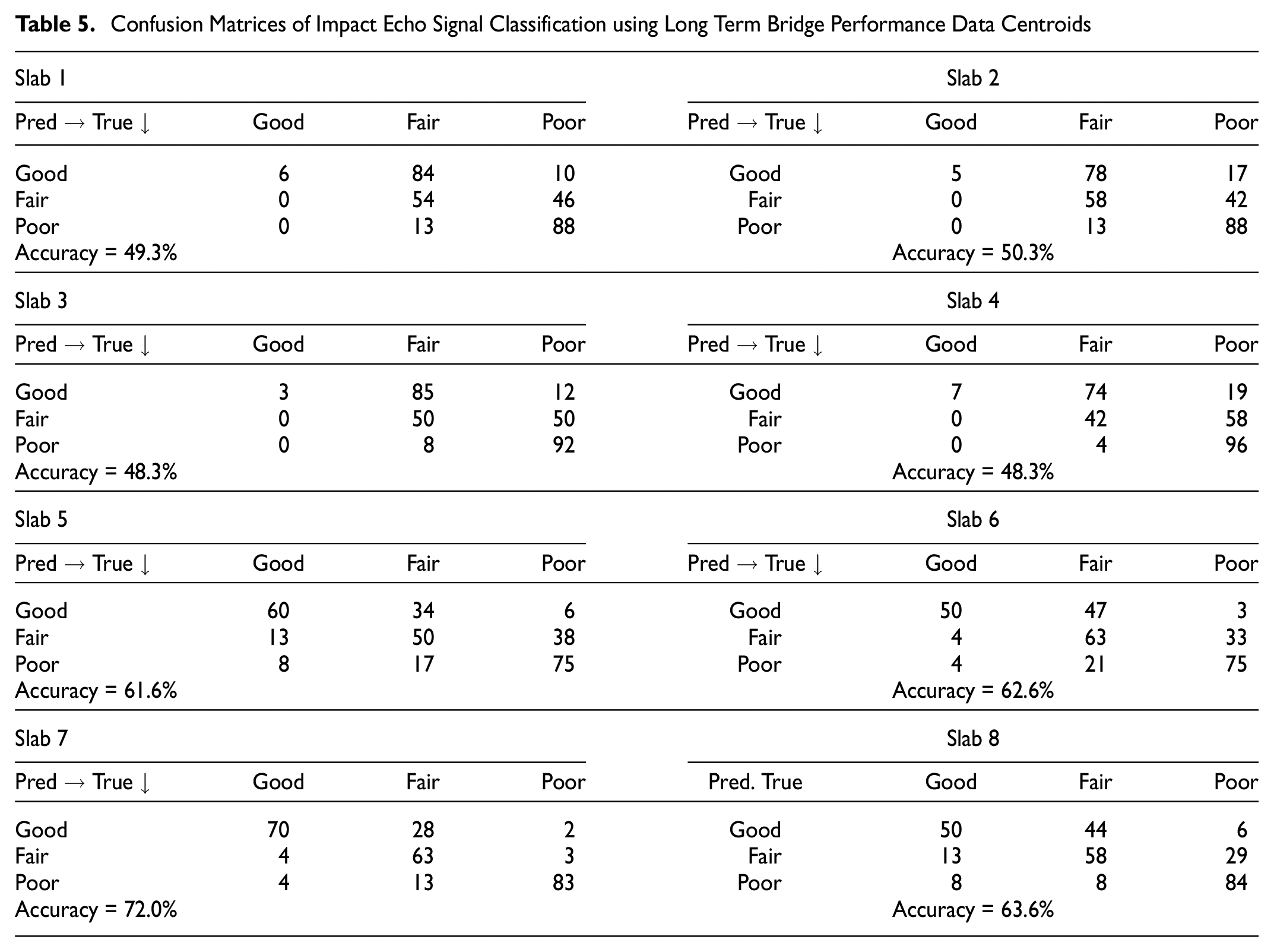
Moreover, the classification performance relies on how signals are grouped into the three classes. As we observe from Figure 5, honeycombing and deep delaminations span through both “poor” and “fair” classes. In fact, there seems to exist a fuzziness to the degree of association to both classes. The centroids obtained from the LTBP dataset are used to classify the experimental data in a similar fashion to compare the transferability of results across different datasets (see Table 5). The results suggest that the classification accuracy remains similar regardless of the dataset used to identify the centroids.

Table 5.

Confusion Matrices of Impact Echo Signal Classification using Long Term Bridge Performance Data Centroids

Slab 1				Slab 2
Pred → True ↓	Good	Fair	Poor	Pred → True ↓	Good	Fair	Poor
Good	6	84	10	Good	5	78	17
Fair	0	54	46	Fair	0	58	42
Poor	0	13	88	Poor	0	13	88
Accuracy = 49.3%				Accuracy = 50.3%
Slab 3				Slab 4
Pred → True ↓	Good	Fair	Poor	Pred → True ↓	Good	Fair	Poor
Good	3	85	12	Good	7	74	19
Fair	0	50	50	Fair	0	42	58
Poor	0	8	92	Poor	0	4	96
Accuracy = 48.3%				Accuracy = 48.3%
Slab 5				Slab 6
Pred → True ↓	Good	Fair	Poor	Pred → True ↓	Good	Fair	Poor
Good	60	34	6	Good	50	47	3
Fair	13	50	38	Fair	4	63	33
Poor	8	17	75	Poor	4	21	75
Accuracy = 61.6%				Accuracy = 62.6%
Slab 7				Slab 8
Pred → True ↓	Good	Fair	Poor	Pred. True	Good	Fair	Poor
Good	70	28	2	Good	50	44	6
Fair	4	63	3	Fair	13	58	29
Poor	4	13	83	Poor	8	8	84
Accuracy = 72.0%				Accuracy = 63.6%

Using the signal classification scheme (and experimental data centroids), the condition maps for the eight slabs are generated as shown in Figure 7, where the different in-built defects can be clearly identified. However, as before, deep delamination is not accurately identified in all cases. Moreover, the condition maps generated using LTBP data (Figure 8) centroids are similar to the ones presented using experimental data.

Figure 7.

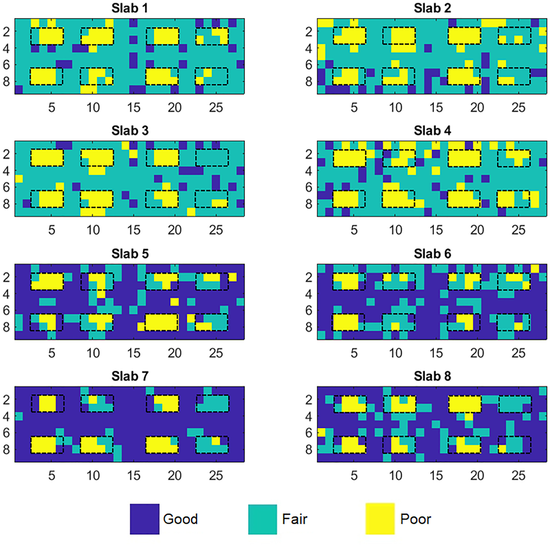
Condition map using laboratory data centroids.

Figure 8.

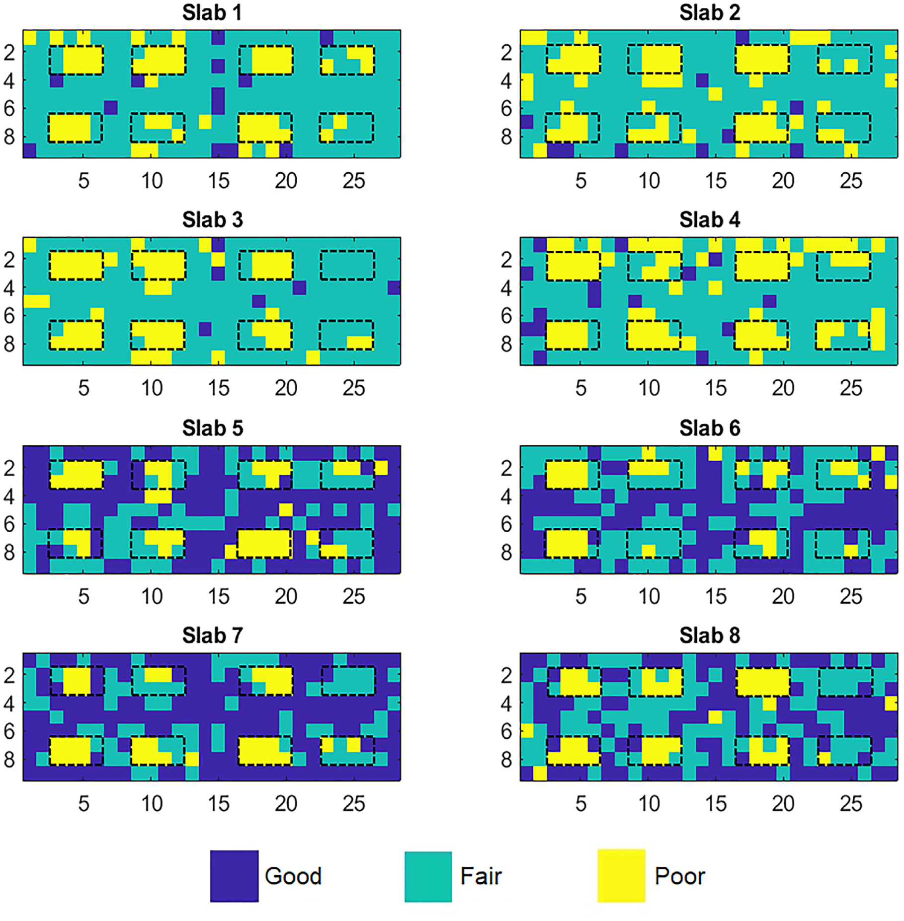
Condition map using Long Term Bridge Performance data centroids.

The proposed method uses an unsupervised clustering on energy proportions in different frequency bands as features to identify class centroids. In addition, the frequency bands are defined relative to the thickness resonance of the deck slab. Therefore, this approach does not depend on the specifics of the bridge deck itself, that is, signals with the same condition would still be identified correctly even if the thickness resonances of the decks are different. Therefore, the proposed methodology is robust and suitable for transfer learning.

Conclusions

IE is an acoustic nondestructive testing method that is used to identify defects in concrete structures such as bridge decks. Researchers have proposed various data-driven models for autonomous interpretation of IE signals to infer subsurface defects that might not be visible from visual inspection methods. IE signals belonging to different defect locations show distinct spectral characteristics that hint at the degree of subsurface damage. In Sengupta et al. ( 23 ), the authors proposed a frequency partitioning of the IE spectrum for autonomous classification into three classes—“good,”“fair,” and “poor.” This classification scheme was developed using real bridge data from the FHWA LTBP dataset that were unlabeled (i.e., without ground truth). In this study, we present a validation of the physics-based classification scheme on an experimental dataset with known defects. Results indicate that the classification method is robust and can classify signals with moderate accuracy. As expected, shallow delamination and voids are most accurately identified, while honeycombing and deep delamination are misclassified. These defects are often difficult to isolate from “no defect” points because of the limitations in the spectral approach. Often, these defects have different degrees of association with the three classes and therefore assigning a particular class is not well justified. In such cases, a fuzzy classification approach could be used as an appropriate alternative, which will be explored in future studies.

Footnotes

Acknowledgements

The experimentation was performed at the FHWA, Turner Fairbank Highway Research Center.

Author Contributions

The authors confirm contribution to the paper as follows: study conception and design: A. Sengupta, H. Azari, S. I. Guler, P. Shokouhi; data collection: H. Azari; analysis and interpretation of results: A. Sengupta, H. Azari, S. I. Guler, P. Shokouhi; draft manuscript preparation: A. Sengupta, H. Azari, S. I. Guler, P. Shokouhi. All authors reviewed the results and approved the final version of the manuscript.

Declaration of Conflicting Interests

The author(s) declared no potential conflicts of interest with respect to the research, authorship, and/or publication of this article.

Funding

The author(s) disclosed receipt of the following financial support for the research, authorship, and/or publication of this article: This work was partially supported by the funds available through Institute for Computational and Data Sciences Seed Grant 2021-22, The Pennsylvania State University.

ORCID iDs

Agnimitra Sengupta

Hoda Azari

S. Ilgin Guler

Parisa Shokouhi

References

Hoegh

Khazanovich

Dai

Evaluating Asphalt Concrete Air Void Variation via GPR Antenna Array Data. Case Studies in Nondestructive Testing and Evaluation, Vol. 3, 2015, pp. 27–33.

Huston

Cui

Burns

Hurley

Concrete Bridge Deck Condition Assessment with Automated Multisensor Techniques. Structure and Infrastructure Engineering, Vol. 7, No. 7-8, 2011, pp. 613–623.

McDaniel

Celaya

Nazarian

Concrete Bridge Deck Quality Mapping with Seismic Methods: Case Study in Texas. Transportation Research Record: Journal of the Transportation Research Board, 2010. 2202: 53–60.

Scott

Rezaizadeh

Delahaza

Santos

Moore

Graybeal

Washer

A Comparison of Nondestructive Evaluation Methods for Bridge Deck Assessment. NDT & E International, Vol. 36, No. 4, 2003, pp. 245–255.

Sultan

A. A.

Washer

G. A.

Comparison of Two Nondestructive Evaluation Technologies for the Condition Assessment of Bridge Decks. Transportation Research Record: Journal of the Transportation Research Board, 2018. 2672: 113–122.

Kee

S.-H.

Arndt

R. W.

Popovics

J. S.

Zhu

Comparison of NDT Methods for Assessment of a Concrete Bridge Deck. Journal of Engineering Mechanics, Vol. 139, No. 3, 2013, pp. 305–314.

Pospisil

Manychova

Stryk

Korenska

Matula

Svoboda

Diagnostics of Reinforcement Conditions in Concrete Structures by GPR, Impact-Echo Method and Metal Magnetic Memory Method. Remote Sensing, Vol. 13, No. 5, 2021, p. 952.

Layssi

Ghods

Alizadeh

A. R.

Salehi

Electrical Resistivity of Concrete. Concrete International, Vol. 37, No. 5, 2015, pp. 41–46.

Leelalerkiet

Kyung

J.-W.

Ohtsu

Yokota

Analysis of Half-Cell Potential Measurement for Corrosion of Reinforced Concrete. Construction and Building Materials, Vol. 18, No. 3, 2004, pp. 155–162.

10.

Maierhofer

Nondestructive Evaluation of Concrete Infrastructure with Ground Penetrating Radar. Journal of Materials in Civil Engineering, Vol. 15, No. 3, 2003, pp. 287–297.

11.

Carino

N. J.

Sansalone

Hsu

N. N.

Flaw Detection in Concrete by Frequency Spectrum Analysis of Impact-Echo Waveforms. In International Advances in Nondestructive Testing ( McGonnagle

W. J.

, ed.), Gordon and Breach, New York, 1986, pp. 117–146.

12.

Carino

N. J.

Sansalone

Impact-Echo: A New Method for Inspecting Construction Materials. Proc., Conference on NDT&E Manufacturing Construction, University of Illinois at Urbana–Champaign, 1988, pp. 209–223.

13.

Sansalone

Carino

N. J.

Detecting Delaminations in Concrete Slabs With and Without Overlays Using the Impact-Echo Method. ACI Materials Journal, Vol. 86, No. 2, 1989, pp. 175–184.

14.

Sansalone

Streett

W. B.

Impact-Echo: Nondestructive Evaluation of Concrete and Masonry. Bullbrier Press, Ithaca, NY, 1997.

15.

Gucunski

Nondestructive Testing to Identify Concrete Bridge Deck Deterioration. National Research Council, Transportation Research Board, Second Strategic Highway Research Program. Transportation Research Board, Washington, D.C., 2013.

16.

Cao

Xiao

Zhang

Wang

Robotic Impact-Echo Non-Destructive Evaluation Based on FFT and SVM. Proc., 11th World Congress on Intelligent Control and Automation, Shenyang, China, IEEE, New York, 2014, pp. 2854–2859.

17.

Luk

B. L.

Liu

Jiang

Tong

Robotic Impact-Acoustics System for Tile-Wall Bonding Integrity Inspection. Mechatronics, Vol. 19, No. 8, 2009, pp. 1251–1260.

18.

Pratt

The Use of a Neural Network for Automating Impact-Echo Signal Analysis. Materials Journal of the American Concrete Institute, Vol. 89, 1992, pp. 178–187.

19.

Sadowski

Non-Destructive Identification of Pull-Off Adhesion Between Concrete Layers. Automation in Construction, Vol. 57, 2015, pp. 146–155.

20.

Zhang

J.-K.

Yan

Cui

D.-M.

Concrete Condition Assessment Using Impact-Echo Method and Extreme Learning Machines. Sensors, Vol. 16, No. 4, 2016, p. 447.

21.

Dorafshan

Azari

Evaluation of Bridge Decks with Overlays Using Impact Echo, a Deep Learning Approach. Automation in Construction, Vol. 113, 2020, p. 103133.

22.

Dorafshan

Azari

Deep Learning Models for Bridge Deck Evaluation Using Impact Echo. Construction and Building Materials, Vol. 263, 2020, p. 120109.

23.

Sengupta

Ilgin Guler

Shokouhi

Interpreting Impact Echo Data to Predict Condition Rating of Concrete Bridge Decks: A Machine-Learning Approach. Journal of Bridge Engineering, Vol. 26, No. 8, 2021, p. 04021044.

24.

Lin

Azari

Meng

Shams

Nondestructive Evaluation of Concrete Bridge Decks with Overlays. U.S. Federal Highway Administration, Office of Infrastructure Research and Development, McLean, VA, 2021.

25.

Hartigan

J. A.

Wong

M. A.

Algorithm AS 136: A K-Means Clustering Algorithm. Journal of the Royal Statistical Society. Series C (Applied Statistics), Vol. 28, No. 1, 1979, pp. 100–108.

Validating a Physics-Based Automatic Classification Scheme for Impact Echo Signals on Data Using a Concrete Slab with Known Defects

Abstract

Keywords

Data Description

Methodology

Estimating the Thickness Resonance Bandwidth

Partitioning the IE Power Spectrum

Classification of IE Signals

Results and Discussion

Conclusions

Footnotes

Acknowledgements

Author Contributions

Declaration of Conflicting Interests

Funding

ORCID iDs

References