Real-Time Intersection Turning Movement Flow Forecasting Using a Parallel Bidirectional Long Short-Term Memory Neural Network Model

Abstract

Real-time forecasting of intersection turning movements is a critical requirement for predictive traffic signal control at signalized intersections. Several traffic flow forecasting models have been developed in the past; however, most of them have focused only on the road segment-level traffic instead of the turning movement flow (TMF) at intersections. Therefore, in this paper, we propose a new TMF forecasting model, which consists of a combination of two neural network models, namely the stacked bidirectional long short-term memory and the traditional multi-layer perceptron model; this combination will enable effective learning for both short- and long-term time-varying patterns. Moreover, extensive computational experiments, using two years of turning movement counts at 22 intersections in the city of Milton, Ontario, Canada, explore the performance advantage of the proposed model in comparison with several state-of-the-art base models for forecasting accuracy, robustness, and transferability.

Real-time traffic flow forecasting is a critical component of many advanced traffic management and information systems (ATMS/ATISs). Moreover, accurate forecasting of intersection traffic can enable the prediction of traffic signal control and timing to improve traffic operations and safety. As for road users, accurate and timely information on future traffic congestion can help in making their travel-related decisions, such as where, when, and in what mode/direction to travel.

In the past decade, several traffic forecasting models have been developed, ranging from statistical time-series models, such as the autoregressive integrated moving average (ARIMA), to machine learning (ML) algorithms, such as long short-term memory (LSTM). Nevertheless, a limited number of previous studies have focused on the problem of real-time forecasting of turning movement flows (TMFs). Therefore, through this research, we will try to address this challenge by taking advantage of the latest advances in the field of machine learning (ML), especially deep neural networks (DNN). We propose a novel parallel bidirectional LSTM model (PB-LSTM) which integrates two proven DNN models, namely, the stacked bidirectional LSTM model (SBiLSTM) ( 1 ) and the traditional multi-layer perceptron model (MLP). SBiLSTM is effective in capturing short-term dynamics of data, while MLP is efficient in incorporating other influencing factors and learning throughout the long-term priority of the data. To the best of our knowledge, this paper represents the first attempt to introduce the PB-LSTM model architecture for traffic flow forecasting, in general, and intersection TMFs forecasting, in particular. Moreover, this research is among the few to train and evaluate a forecasting model using a large real-world turning movement counts (TMCs) dataset. An extensive set of computational experiments is conducted, providing valuable insights into several critical questions associated with the model, such as how does the performance of the proposed model vary by using various model settings such as the input data range and the forecasting horizon? Is it possible to improve the performance and transferability of the proposed model by incorporating additional features or by performing location clustering?

To sum up, the remainder of this paper proceeds as follows: the literature review section reviews the classical, ML, and Deep Learning (DL)-based traffic prediction models. The methodology section details the proposed model, followed by the case study section with various experiments relative to the sensitivity analysis. The results section discusses the experimental findings. Finally, the main results and directions for future research are discussed in the conclusion section.

Literature Review

The problem of short-term traffic flow forecasting has been studied extensively in the transportation engineering field. Different forecasting models have been developed, ranging from the traditional statistical time-series models to the latest DL models. The most popular classical statistical model for time-series prediction is ARIMA ( 2 ). Researchers have applied ARIMA and its variants, such as the seasonal ARIMA ( 3 ) and ARIMAX ( 4 ) models, for traffic forecasting. Another statistical model, Prophet, is proposed by Facebook for time-series forecasting ( 5 ). It is based on an additive model where nonlinear trends are fit with annual, weekly, and daily seasonality, as well as holiday effects. For instance, Chikkakrishna et al. ( 6 ) applied seasonal ARIMA and Prophet models separately for short-term traffic forecasting. They found that the Prophet model can make use of unsmoothed data for traffic forecasting with lower and upper bounds.

Zhang et al. ( 7 ) applied the K-nearest neighbors (KNN) method for short-term traffic flow prediction and showed good performance results. Moreover, Smith and Demetsky ( 8 ) compared ARIMA with KNN and showed that KNN outperformed ARIMA based on the average absolute error value.

In addition to KNN, other ML algorithms, such as support vector regression (SVR), the random forest (RF), and the traditional MLP, have also been explored for traffic forecasting. For example, Liu and Wu ( 9 ) proposed an RF model to predict traffic flow and congestion. Their result showed that the accuracy of the model was as high as 87.5% in predictions of congestion. Furthermore, Leshem et al. ( 10 ) conducted a performance analysis and found that the SVR method has a superior performa1nce compared with other time-series models as its root mean square error (RMSE) for a 1 min aggregation interval traffic count prediction is only 0.42 vehicle per minute. Compared with the single regressor, AdaBoost—which is an ensemble of learning models consisting of plentiful weak regressors—has shown better forecasting performance, more specifically 60% better than KNN and SVR ( 10 ).

With the development of several ML techniques, the performance of traffic forecasting has improved significantly over the years. This is especially true with the latest DL models such as the convolutional neural networks (CNNs), which are capable of dealing with a variety of large datasets ( 11 , 12 ). Recently, the application of recurrent neural networks (RNNs) in time-series analysis has become dominant. In more detail, RNNs are neural networks with hidden states which keep the previous time features for modeling sequential data. For instance, Van Lint et al. ( 13 ) applied RNNs to model the freeway travel time, and their model was found to outperform other forward ML algorithms by around 10% better with a 72% smaller model size. Moreover, LSTM models, an improved variant of RNN with improved long-term and short-term temporal learning features, reached an excellent ability for traffic forecasting ( 14 , 15 ). Having the same input historical data length, LSTM achieved 37.5% less RMSE than the SVR model ( 14 , 15 ). The LSTM model was recently extended to the BiLSTM to capture the forward and backward dependencies in typical traffic time-series data, showing a significant performance enhancement ( 16 ). In addition, attempts have also been made to integrate CNN along with the LSTM model to account for some additional features like the number of lanes and the occupancies in forecasting. This new model achieved a prediction RMSE that reached around 10 vehicles per hour per lane ( 17 ).

Despite the significant progress in traffic forecasting, the problem of intersection turning movement forecasting has received very limited attention. Most previous efforts have focused on predicting turning movements using highly aggregated origin-destination (O-D) data ( 18 , 19 ). For instance, Karnati et al. ( 20 ) developed a simple NN-based model on TMCs data from a SUMO simulation model and showed that a three-layer simple NN-based model performed very well with 0.001 mean squared error per 375 s in both oversaturated and undersaturated conditions for predicting the next 375 s TMFs. Moreover, Ghanim et al. ( 21 ) developed an MLP model, a fully connected class of feedforward ANN that generates a set of outputs based on a set of inputs. Although their results showed that their model performed exceptionally well, there are several limitations in their studies, among them: (i) the dataset resolution is low, and it only covers peak hours, limiting the application of their model; (ii) the turning movement data was processed as simple cross-sectional observations instead of time series, ignoring the potential autocorrelation and periodicity in the traffic data.

Methodology

Proposed Model

In this study, the time series of D movements at an intersection is denoted as $X={[{\mathit{x}}_1,{\mathit{x}}_2,\dots ,{\mathit{x}}_{\mathit{T}}]}^T\in R^{T\times D}$ with $T$ representing the time steps, where ${\mathit{x}}_{\mathit{t}}$ is a vector ( ${\mathit{x}}_{\mathit{t}}$  =  $[x_t^1,$ $x_t^2,\dots ,$ $x_t^D]$ ) denoting the movement flows at time t. The intersection movement flow prediction problem is defined as learning a function F(·) to map T historical TMFs to the TMFs workspace at a specific prediction horizon, $\Delta \mathit{t}$ . Therefore, the following expression can be obtained:

$$[{\mathit{x}}_{\mathit{T}+\Delta \mathit{t}}]=\mathit{F}\left([{\mathit{x}}_1,{\mathit{x}}_2,\dots ,{\mathit{x}}_{\mathit{T}}]\right)$$

(1)

As described in the previous section, many traffic flow forecasting models (i.e., function F(·)) have been developed in the literature, having different fundamental model structures, assumptions on data availability, and application environments. However, our proposed model, the PB-LSTM, is a DNN model built on two well-known NN models, namely, LSTM and MLP. The LSTM model ( 22 )has been successfully applied for time-series forecasting with long-term dependencies ( 1 , 17 , 23 , 24 ). Furthermore, over the past few years, many different forms of LSTM have been proposed for traffic flow forecasting; however, none has shown significant performance improvement over the basic LSTM model ( 17 ). This latter consists of a sequence of processing cells of the same structure, as shown in Figure 1. The input of the LSTM cell includes several parameters: $x_t$ which represents the current variable vector, $h_{t-1}$ indicating the preceding output, and $C_{t-1}$ presenting the initial cell state. Moreover, the cell state is the key to LSTM: it runs straight down the entire chain to keep the long-term information unchanged, with only minor linear interactions. When there is a need to remove or add information to the cell state, the LSTM provides three gates to protect and control such cells. The first gate (refer to Equation 2) represents the forgotten gate, and it helps to decide what information to filter out from the previous one. It evaluates $h_{t-1}$ and $x_t$ , and generates a number between 0 and 1 for each number in the cell state $C_{t-1}$ . The next step consists of deciding what new information to store in the cell gate, as mentioned in Equations 3 and 4. The input gate, including the sigmoid layer, determines which values to update, and a tanh layer creates a vector of the new candidate values, ${\tilde{C}}_t$ . After that, the old cell state, $C_{t-1}$ , will be updated into the new cell state, $C_t$ (refer to Equation 5). In the last step, the sigmoid layer will decide what parts of the state to output, and then the output will pass through the tanh layer and multiply the cell state as shown in Equations 6 and 7.

Figure 1.

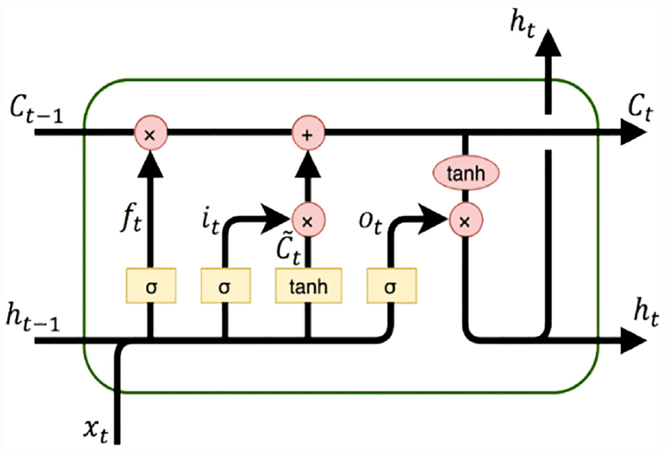
Structure of the basic long short-term memory (LSTM) cell ( 23 ).

$${\mathit{f}}_{\mathit{t}}=\sigma ({\mathit{W}}_{\mathit{f}}·[{\mathit{h}}_{\mathit{t}-1},{\mathit{x}}_{\mathit{t}}]+{\mathit{b}}_{\mathit{f}})$$

(2)

$${\mathit{i}}_{\mathit{t}}=\sigma ({\mathit{W}}_{\mathit{i}}·[{\mathit{h}}_{\mathit{t}-1},{\mathit{x}}_{\mathit{t}}]+{\mathit{b}}_{\mathit{i}})$$

(3)

$${\tilde{\mathit{C}}}_{\mathit{t}}=\tanh ({\mathit{W}}_{\mathit{C}}·[{\mathit{h}}_{\mathit{t}-1},{\mathit{x}}_{\mathit{t}}]+{\mathit{b}}_{\mathit{C}})$$

(4)

$${\mathit{C}}_{\mathit{t}}={\mathit{f}}_{\mathit{t}}\times {\mathit{C}}_{\mathit{t}-1}+{\mathit{i}}_{\mathit{t}}\times {\tilde{\mathit{C}}}_{\mathit{t}}$$

(5)

$${\mathit{o}}_{\mathit{t}}=\sigma ({\mathit{W}}_{\mathit{o}}·[{\mathit{h}}_{\mathit{t}-1},{\mathit{x}}_{\mathit{t}}]+{\mathit{b}}_{\mathit{o}})$$

(6)

$${\mathit{h}}_{\mathit{t}}={\mathit{o}}_{\mathit{t}}\times \tanh \left({\mathit{C}}_{\mathit{t}}\right)$$

(7)

Furthermore, multiple basic LSTM cells could be combined in a sequence to form new powerful unidirectional LSTM models. Moreover, they may be set up as two distinct LSTMs that analyze a stream of data in both forward and backward directions, as shown in Figure 2. The resulting model, that is, the SBiLSTM, has been shown to be substantially better than the unidirectional LSTM model ( 24 ). Furthermore, this model can be built as a stacked multi-layer form, resulting in a stacked SBiLSTM ( 25 ). In such an architecture ( 25 ), the output of a hidden layer will be fed as the input into the subsequent hidden layer; this approach has been found to be effective in dealing with certain types of tasks.

Figure 2.

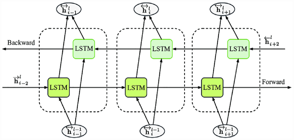
Stacked bidirectional long short-term memory (SBiLSTM) structure.

To sum up, in this study, an additional MLP layer is added to the top of the stacked SBiLSTM to capture the potential interactions between the individual movements at an intersection. The latter represents information with long-term relevance (e.g., the memory). The resulting model is known as the PB-LSTM model, as shown in Figure 3. The combination of the MLP and SBiLSTM structures is expected to make full use of both time-series and non-time-series data and enable both short-term and mid-term forecasting. Moreover, each record includes two parts, $X_{\mathrm{TMC}}$ and $X_{\mathrm{stamp}}$ . In the upper part data, $X_{\mathrm{TMC}}$ is TMCs time-series data for the $D$ traffic movements, and each record indicates the aggregation count of 5 min volume. This part of the data is processed by the SBiLSTM block: the first layer of the SBiLSTM block represents the time-distributed dense layer which is used to capture the inner relationship of the traffic movements for every temporal input value, and the process will not eliminate time dependence when capturing the TMCs dependencies. Moreover, the subsequent three stacked layers are LSTM layers with 32 units, and they will analyze the time dependency for each movement. There is another feature of data $X_{\mathrm{stamp}}$ , processed by an MLP block including hours of the day, day of the week, the month of the year, and intersection clustering label from the KNN model (which will be described in detail throughout this paper); therefore, the MLP block consists of three dense layers with each having 16 units with the Relu ( 16 ) activation function. After the two blocks, the 1-D output vectors from $X_{\mathrm{TMC}}$ and $X_{\mathrm{stamp}}$ are concatenated together and passed to the dense layer to make the final prediction.

Figure 3.

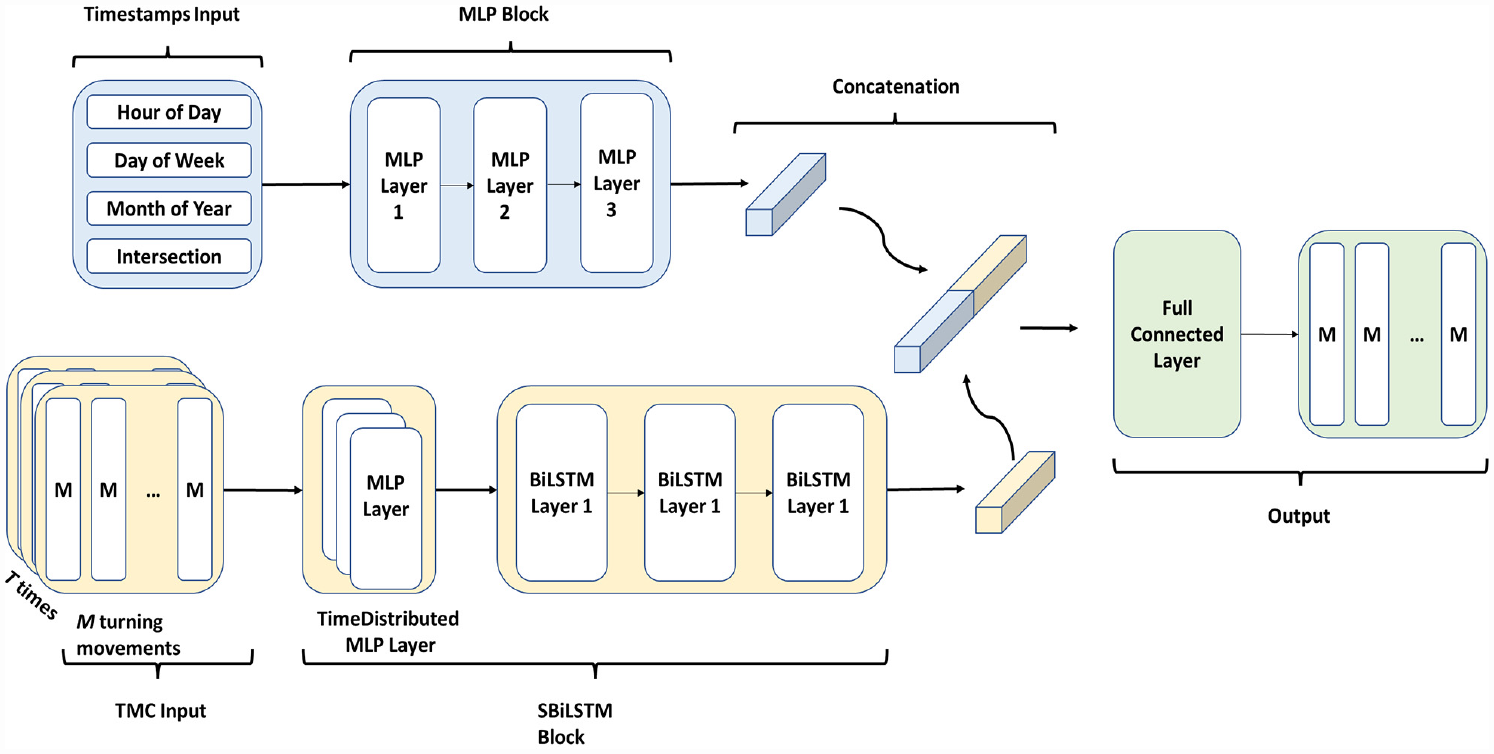
Summary of parallel bidirectional long short-term memory model (PB-LSTM) model.

Case Study Data Description

A case study is conducted to evaluate the performance of the proposed PB-LSTM model and compare it with several existing state-of-the-art models. The dataset used in the study includes TMCs measured at 5 min intervals regrouping 49 signalized intersections in Milton, Ontario, Canada, for the period from 2019 to 2021 (as shown in Figure 4). The TMCs were collected using the Miovision SmartSense system, whose main features are summarized in Table 1.

Figure 4.

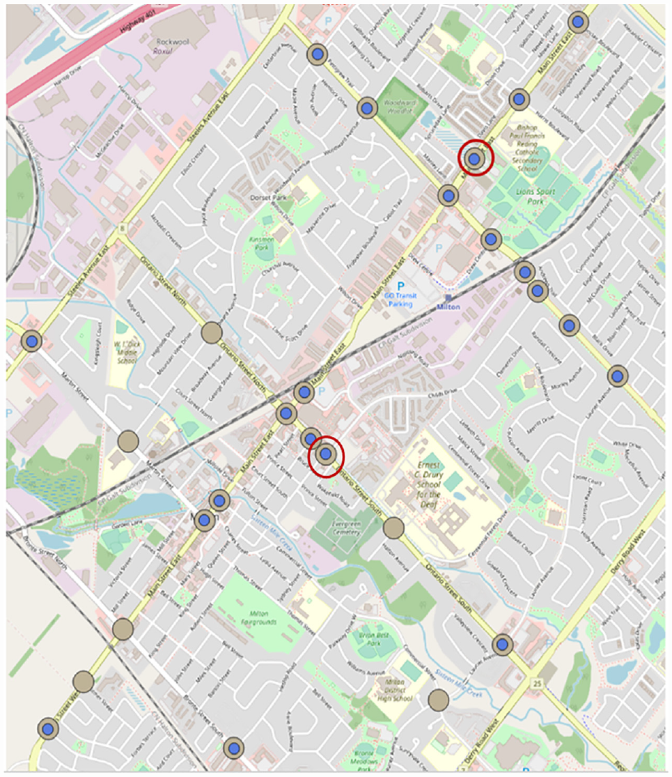
Case study intersections. The brown dots are the intersections being monitored, the blue dots are the intersections selected for analysis, and the intersections in the red circle are additional test intersections.

Table 1.

Features Included in the Raw Data

Type	Features
Movement	TH (Through traffic)	LT (Left turn plus U-turn)	RT (Right turn)
Counts	Counts of each record
Location	Latitude	Longitude	NA
Time	Hour of day	Day of week	Month of year

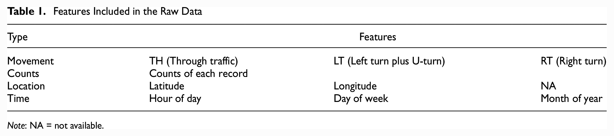
Note: NA = not available.

In this study, 20 intersections were selected, being those having the most complete data coverage between January 2020 and April 2022. The dataset has a total of 4,901,760 records, which is equal to 245,088 records per intersection. Moreover, the dataset is split randomly into two subsets: 80% for model training and 20% for model testing.

An exploratory data analysis was conducted on a sample intersection (Main Street East and Maple/Sinclair Drive). As a typical time-series dataset, TMCs records englobe daily and weekly seasonality and monthly tendency. Therefore, Figure 5 shows the total 5 min volume of the eastbound approach daily count from January 2020 to April 2022. Based on this figure, the trend over the first year is clearly visualized: the traffic has the first peak at the end of March after continuously growing from January, but it then starts falling until May; after May, the TMC keeps increasing to reach the second peak in September, and then decreases slightly until December. Compared with 2021 and 2022, these noticeable variations in traffic in 2020 were caused by a provincial-wide lockdown in Ontario during these months because of the COVID-19 pandemic; for this reason, we observe rapidly decreasing traffic in April 2020, and it slightly decreases again in October 2020.

Figure 5.

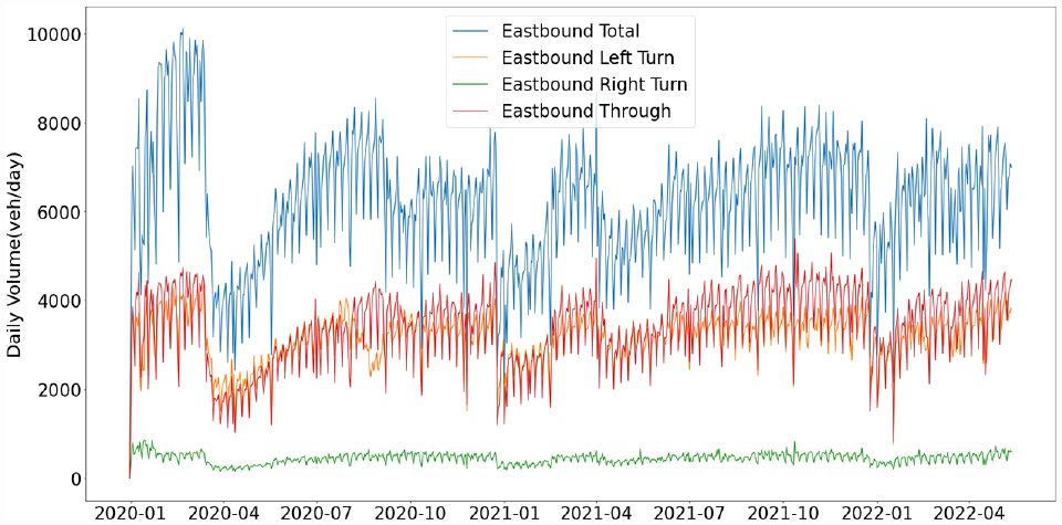
Daily traffic movement counts (TMCs) over the analysis period.

This data analysis has shown the influence of the COVID-19 pandemic on TMCs and confirmed the expected shorter temporary variation patterns in the TMFs, such as daily and weekly seasonality. To identify these time-varying patterns, it is necessary to apply models that can capture both the short-term and the long-term traffic dynamics, such as the proposed PB-LSTM.

Computational Experiments and Results

The proposed PB-LSTM model, along with several base models described in the previous section, was implemented using the Keras backend with Tensor Flow ( 26 ). The DNNs were trained by optimizing the cost function using the Adam method ( 27 ). In the training process, the training dataset was first re-formatted for models to include the input history of a defined length. Moreover, cross-validation was applied at each iteration using 20% of the training dataset selected randomly for model validation. Furthermore, the model parallelism was applied in the computation process: the LSTM and MLP blocks were trained in different Graphics Processing Units (GPUs), and they were then concatenated on the same Central Processing Unit (CPU). The model hyperparameters have been chosen by Bayesian optimization. The average training time for a one-step forecasting is 52 s per iteration on two NVIDIA GeForce GPUs (GTX1080 8GB and GTX1070 8GB), whereas, for the forecasting on the test dataset, 90 s were needed. This implies that each prediction required less than $0.65\times {10}^{-3}$  s. Finally, the following section discusses the main results of several computational experiments.

Preliminary Performance Evaluation

To provide a basis for assessment and comparison, we first implemented several of the most well-known models, including ARIMA ( 28 ), Prophet ( 5 ), linear regression ( 29 ), AdaBoost ( 30 ), RF ( 31 ), MLP ( 32 ), and LSTM ( 33 ) and compared their relative performance. As a preliminary evaluation effort, all models were trained and tested using data measured over a single year (2020) at a given intersection (Main Street East and Maple/Sinclair Drive). The input time-series data range was set to 30 min (i.e., six intervals of 5 min each) and the forecasting horizon 5 min (i.e., next time interval). The performances of the models were evaluated using the average RMSE for all movements at the intersection.

Therefore, Figure 6 shows the RMSE for the forecast TMFs by 5 min traffic volume. For MLP, RF, and AdaBoost, the input is temporarily changing its patterns, including the hour of the day, the day of the week, and the month of the year, whereas LSTM, ARIMA, and Prophet took the same range of observations as input. Moreover, Figure 6 shows that, among all models, LSTM had the best performance, followed by MLP, AdaBoost, and RF, which performed slightly better than the classical models. These results are consistent with the findings from the literature ( 17 ).

Figure 6.

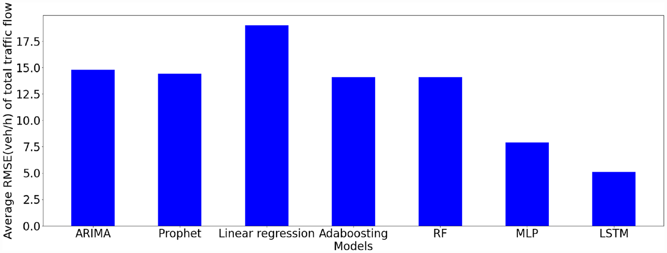
Comparison of the performance of some well-known time-series forecasting models.

Another preliminary computational analysis was conducted to compare the performance of three types of LSTM models, namely, the basic LSTM, the SBiLSTM, and the SBiLSTM with an additional time-distributed full connected perceptron layer (MLP+SBiLSTM). After being combined with the extra MLP layer, SBiLSTM is expected to enhance the forecasting accuracy ( 34 ). These models have been trained using data from the same test intersection and their performance results are shown in Figure 7. It can be observed that SBiLSTM and MLP+SBiLSTM significantly outperformed the basic LSTM, especially at the level of weighted average RMSE. Moreover, the performances of SBiLSTM and MLP+SBiLSTM are relatively close on average RMSE; however, the RMSE of MLP+SBiLSTM for the left- and right-turn movements is lower than SBiLSTM. As a result, the MLP+SBiLSTM model was finally selected for further consideration.

Figure 7.

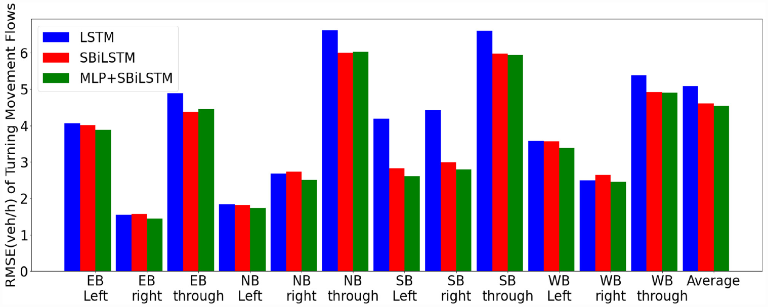
Comparison of forecasting errors of traffic movement flows (TMFs) using the LSTM, SBiLSTM, and MLP+SBiLSTM methods.

The preliminary computational study has shown that both MLP and SBiLSTM models can outperform other models; therefore, they could be used as a building block for constructing new forecasting models such as the proposed PB-LSTM described previously.

Overall Performance

The intersection of Main Street East and Maple/Sinclair Drive is selected for a case study on the overall performance of the PB-LSTM model, with TMCs data covering the period from January 2020 to April 2022. In this experiment, the input data range is 30 min (i.e., six 5 min intervals), whereas the forecasting horizon is 5 min, that is, one interval into the future, which was achieved using a rolling horizon scheme.

Furthermore, Figure 8 shows the forecast intersection daily flows of eastbound traffic by turning movement versus the same as observed for 2020 during the COVID-19 pandemic. In March 2020, the Ontario Government announced the lockdown for the first time; thus, there was a sharp decline in traffic. To sum up, the proposed model successfully captured the general trend of traffic variation over the period.

Figure 8.

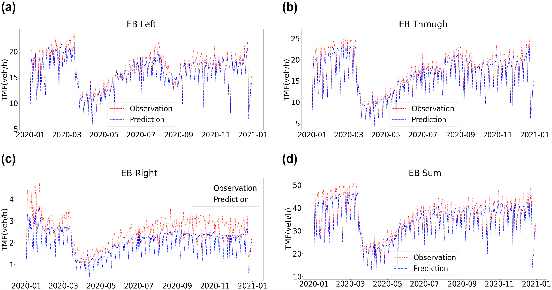
Performance of the PB-LSTM model for forecasting traffic movement flows (TMFs): predicted versus observed daily volume (from January 1, 2020–December 31, 2020 with 30 min input data range and 5 min forecasting horizon): (a) eastbound left, (b) eastbound through, (c) eastbound right, (d) eastbound sum.

Figure 9 shows the forecast intersection flows by turning movement versus the observed flow during weekdays and weekends when testing the dataset between January and December 2020.

Figure 9.

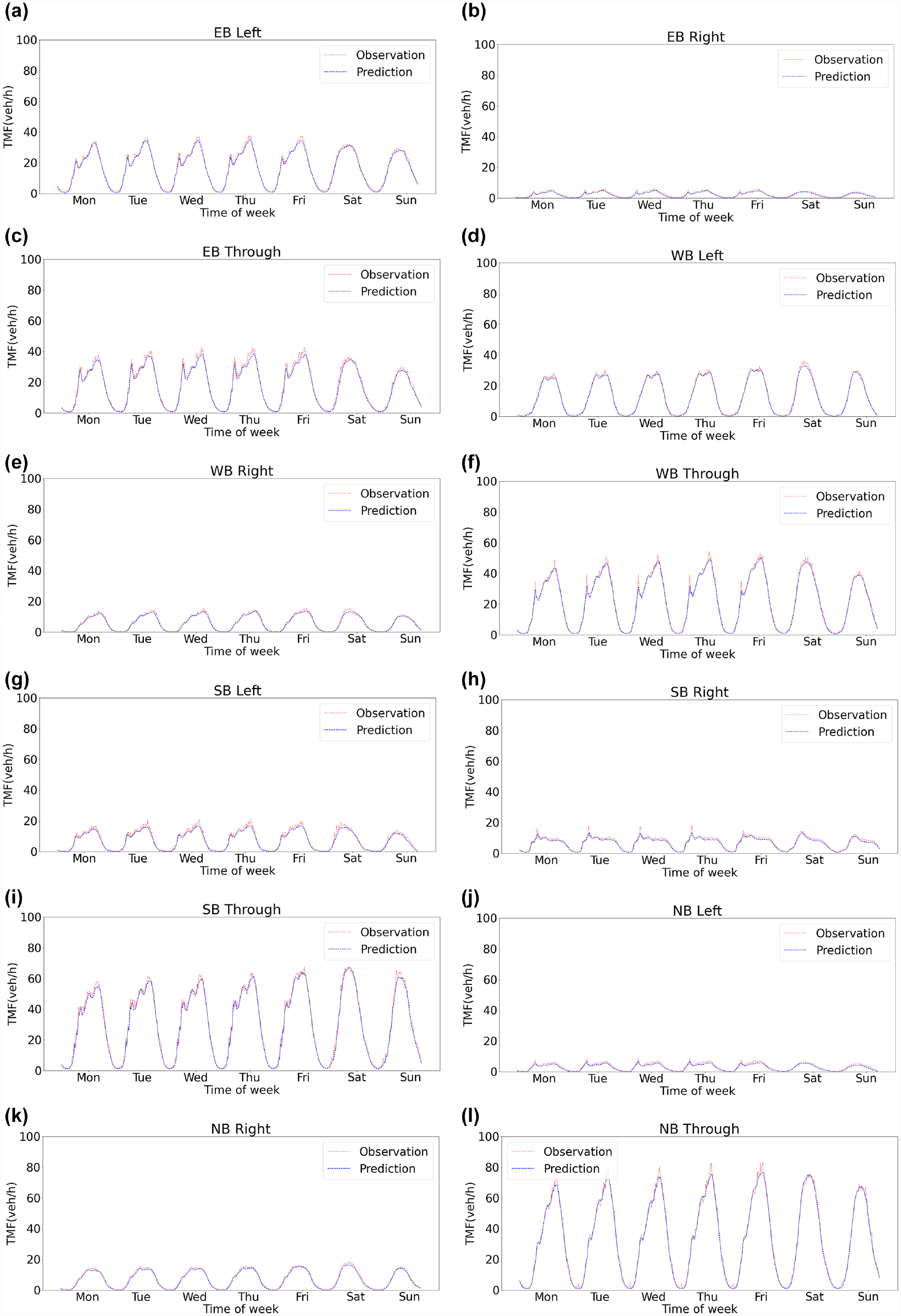
Performance of the PB-LSTM model for forecasting traffic movement flows (TMFs): predicted versus observed 5 min volume (weekdays and weekends, 30 min input data range and 5 min forecasting horizon) (a) eastbound left, (b) eastbound right, (c) eastbound through, (d) westbound left, (e) westbound right, (f) westbound through, (g) southbound left, (h) southbound right, (i) southbound through, (j) northbound left, (k) northbound right, (l) northbound through.

As a result, it can be seen that our proposed model was able to capture the specific traffic daily variations at this intersection accurately. This could be attributed to the integration of the MLP and SBiLSTM models where the former helps in acquiring longer memory (i.e., the daily periodicity) and the latter gains shorter memory for the time-of-day traffic variation. The result shows that the PB-LSTM model was successful in replicating the peaking of most traffic turning movements. However, the forecasting errors appeared to be larger during the peaking points, which is most likely caused by the inherent random variation of traffic, especially when short time intervals (e.g., shorter than 5 min) are considered. Compared with weekday prediction, the performance of TMFs during the weekend only has one peak and the forecasting errors of the PB-LSTM model are much smaller.

Referring to Figures 8 and 9, it can be observed that the PB-LSTM can correctly forecast the trend; however, the predicted counts are lower than the actual ones during high traffic flow conditions. Figure 10 shows the variation of RMSE with respect to the time of day of the PB-LSTM model and SBiLSTM for eastbound traffic for the same intersection while using the testing dataset from January to December 2020. Furthermore, it can be observed that our proposed model outperforms the SBiLSTM model most of the time.

Figure 10.

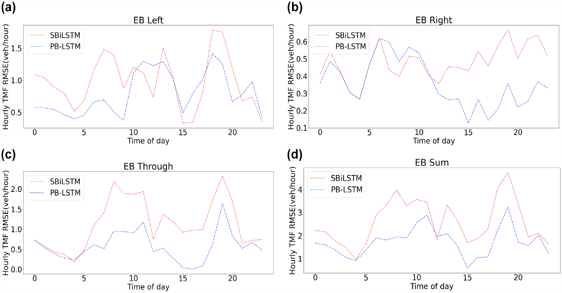
Average root mean square error (RMSE) of the PB-LSTM and SBiLSTM models for forecasting traffic movement flows (TMFs) eastbound (30 min input data range and 5 min forecasting horizon) (a) eastbound left, (b) eastbound through, (c) eastbound right, (d) eastbound sum.

Table 2 shows the performance of our proposed model on 20 intersections for all 12 movements. It is obvious that the prediction error of PB-LSTM is acceptable for all test intersections, as its average is below six vehicles per hour. Moreover, Table 3 compares the performance of our proposed model with SBiLSTM. We can see that the PB-LSTM model outperforms SBiLSTM for all 20 intersections and PB-LSTM has at least 10% less RMSE than SBiLSTM among nine intersections.

Table 2.

Root Mean Square Error of PB-LSTM for Forecasting Traffic Movement Flows of all 20 Intersections

Intersection	Eastbound			Northbound			Southbound			Westbound			Weighted average
	Left	Right	Through	Left	Right	Through	Left	Right	Through	Left	Right	Through
1	1.39	0.92	3.36	0.71	0.41	0.55	1.66	1.59	0.60	0.61	1.41	3.80	2.89
2	0.04	0.03	0.03	0.11	1.58	6.22	1.56	0.13	6.27	1.61	1.61	0.05	5.49
3	1.18	1.77	1.14	1.53	1.67	5.32	1.14	1.34	5.39	1.70	1.19	1.31	4.13
4	0.54	2.33	0.53	2.29	1.90	5.99	0.66	0.63	5.72	1.98	0.56	0.63	4.87
5	2.74	1.00	3.30	1.25	1.70	4.35	1.90	1.87	4.39	2.41	1.65	3.66	3.32
6	1.88	0.04	2.50	0.02	0.02	0.05	0.84	1.96	0.03	0.04	0.97	2.72	2.26
7	0.46	1.04	0.41	1.09	0.82	4.86	0.93	0.57	5.66	0.71	0.97	0.54	4.68
8	0.82	0.05	4.26	0.02	0.02	0.03	0.89	0.71	0.03	0.04	0.79	4.74	4.32
9	2.19	1.95	0.58	1.74	0.55	4.91	0.40	2.09	5.24	0.36	0.63	0.47	4.12
10	1.59	0.06	4.29	0.03	0.03	0.02	1.58	1.55	0.02	0.03	1.78	4.65	3.75
11	0.03	2.07	3.11	2.55	2.20	0.06	0.03	0.04	0.06	2.34	0.03	3.26	2.74
12	0.98	0.74	0.88	0.66	0.95	4.24	1.18	1.03	4.79	1.06	1.27	0.96	3.73
13	2.50	2.24	0.91	2.45	0.81	3.58	0.52	2.32	4.21	0.70	0.53	0.67	3.05
14	1.75	0.08	3.37	3.90	2.84	3.33	1.03	1.60	3.32	3.09	1.22	3.34	3.13
15	1.29	2.22	0.02	1.99	0.09	6.11	0.06	1.28	6.39	0.06	0.04	0.05	5.43
16	0.88	0.78	3.69	0.85	1.10	0.71	1.41	0.78	0.79	1.07	1.24	4.07	3.16
17	2.11	1.85	3.42	1.95	1.30	5.30	1.19	1.97	6.08	1.25	1.14	2.72	4.35
18	3.14	3.05	5.14	1.94	2.37	5.51	2.33	3.24	4.50	1.81	2.10	4.79	4.24
19	0.12	0.97	2.64	1.02	0.89	0.18	0.42	0.16	0.19	0.79	0.22	2.80	2.48
20	4.53	5.33	4.05	2.89	1.50	1.20	1.46	2.59	1.40	1.63	1.50	4.45	3.79

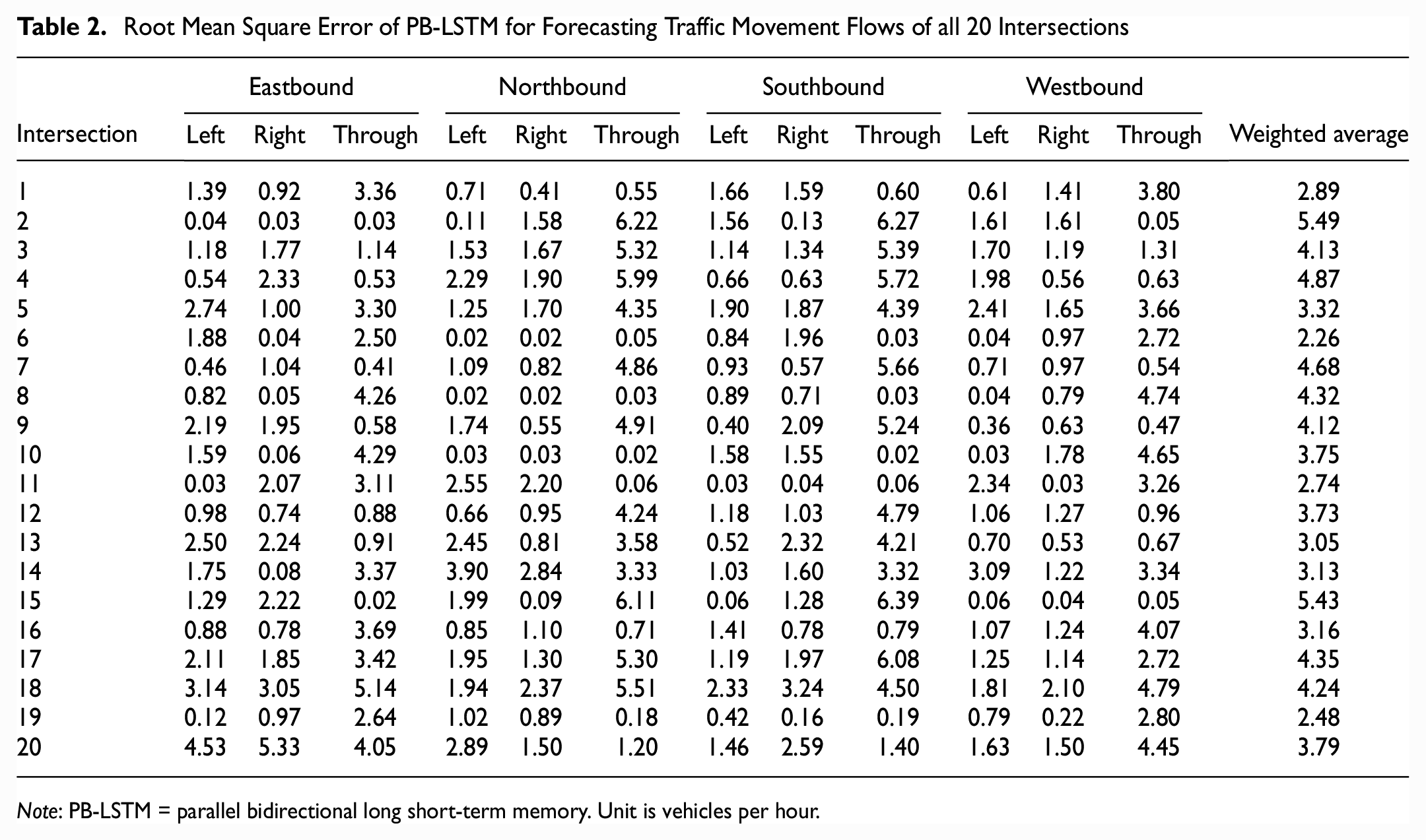
Note: PB-LSTM = parallel bidirectional long short-term memory. Unit is vehicles per hour.

Table 3.

Model Comparison of the Weighted Root Mean Square Error for Forecasting Forecasting Traffic Movement Flows of all 20 Intersections

Intersection	1	2	3	4	5	6	7	8	9	10	11	12	13	14	15	16	17	18	19	20
SBiLSTM	3.16	6.17	4.46	5.71	3.69	2.54	5.03	4.89	4.48	4.12	3.03	4.05	3.27	3.51	6.26	3.53	4.52	4.73	2.71	3.81
PB-LSTM	2.89	5.49	4.13	4.87	3.32	2.26	4.68	4.32	4.12	3.75	2.74	3.73	3.05	3.13	5.43	3.16	4.35	4.24	2.48	3.79
Reduction %	9%	11%	8%	15%	10%	11%	7%	12%	8%	9%	9%	8%	7%	11%	13%	11%	4%	10%	9%	1%

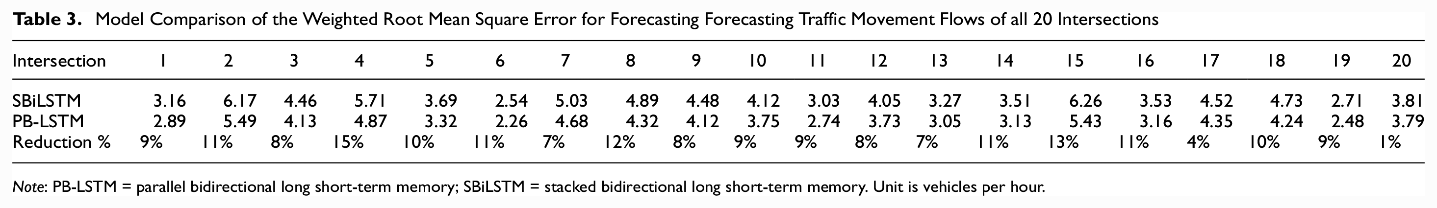
Note: PB-LSTM = parallel bidirectional long short-term memory; SBiLSTM = stacked bidirectional long short-term memory. Unit is vehicles per hour.

Effect of Input Data Range

In this experiment, the proposed model along with the two base models (SBiLSTM and MLP) are compared to predict the next 5 min of TMFs under different input data ranges (past 5 min, 10 min, 30 min, 60 min, and 120 min of observations) using data from the intersection of the Main Street and Leisure Centre Driveway.

Figure 11 shows the performance of the SBiLSTM and PB-LSTM models based on four measurement errors (mean absolute error [MAE], mean absolute percentage error [MAPE], RMSE, and root mean square percentage error [RMSPE]), varied by the length of the input data. Note that the result of the MLP model was not included as its errors are much larger in magnitude. The forecasting errors for both models decreased dramatically when the input data range increased from 5 min to 30 min and then it leveled off. The result also shows that the proposed PB-LSTM needed a shorter length of input data to achieve most of the performance gain compared with the Bi-LSTM model. Therefore, the optimal input data length could be as low as 30 min for the PB-LSTM model and 60 min for the SBiLSTM model. It should also be noted that the proposed PB-LSTM model outperformed the SBiLSTM model consistently under all input data ranges.

Figure 11.

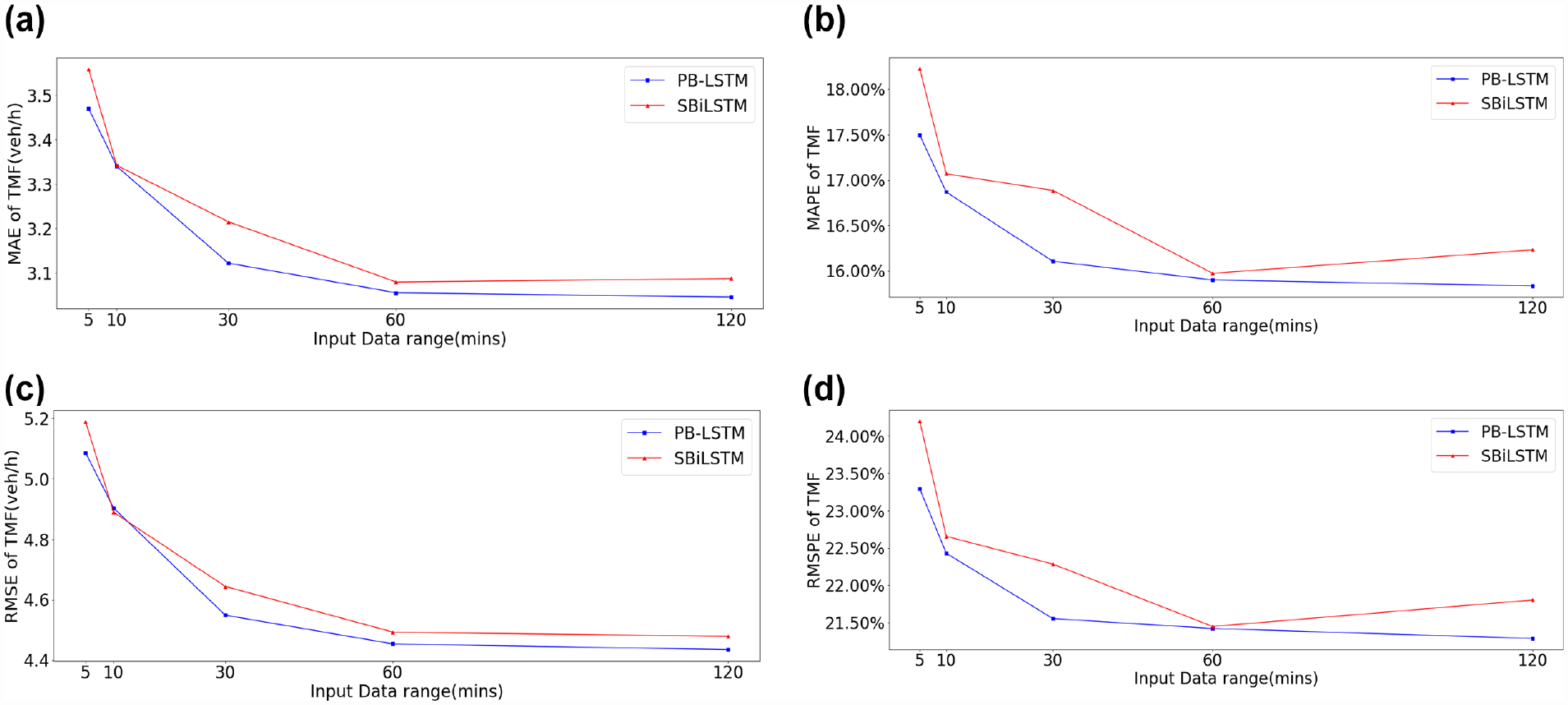
Weighted average performance comparison of two models under different observation range when predicting the next 5 min flow: (a) mean absolute error, (b) mean absolute percent error, (c) root mean square error, (d) root mean square percent error.

Effect of the Forecasting Horizon

The performance of the time-series forecasting models typically deteriorates as the forecasting horizon increases. Therefore, the focus of this section is to determine the underlying performance pattern of the proposed model having, as an objective, the quantification of the speed and magnitude of the deterioration in comparison with the base model. The trained model was thus applied in a rolling horizon to forecast the future traffic movements using the same case study intersection as in the previous experiment with a forecasting horizon ranging from one interval (5 min) to 24 intervals (120 min). Therefore, Figure 12 shows that the forecasting errors of both models (SBiLSTM and PB-LSTM) increased approximately in a linear way by the forecasting horizon. However, the proposed model showed a clear performance advantage over the SBiLSTM model in both the error magnitude and the performance deterioration speed.

Figure 12.

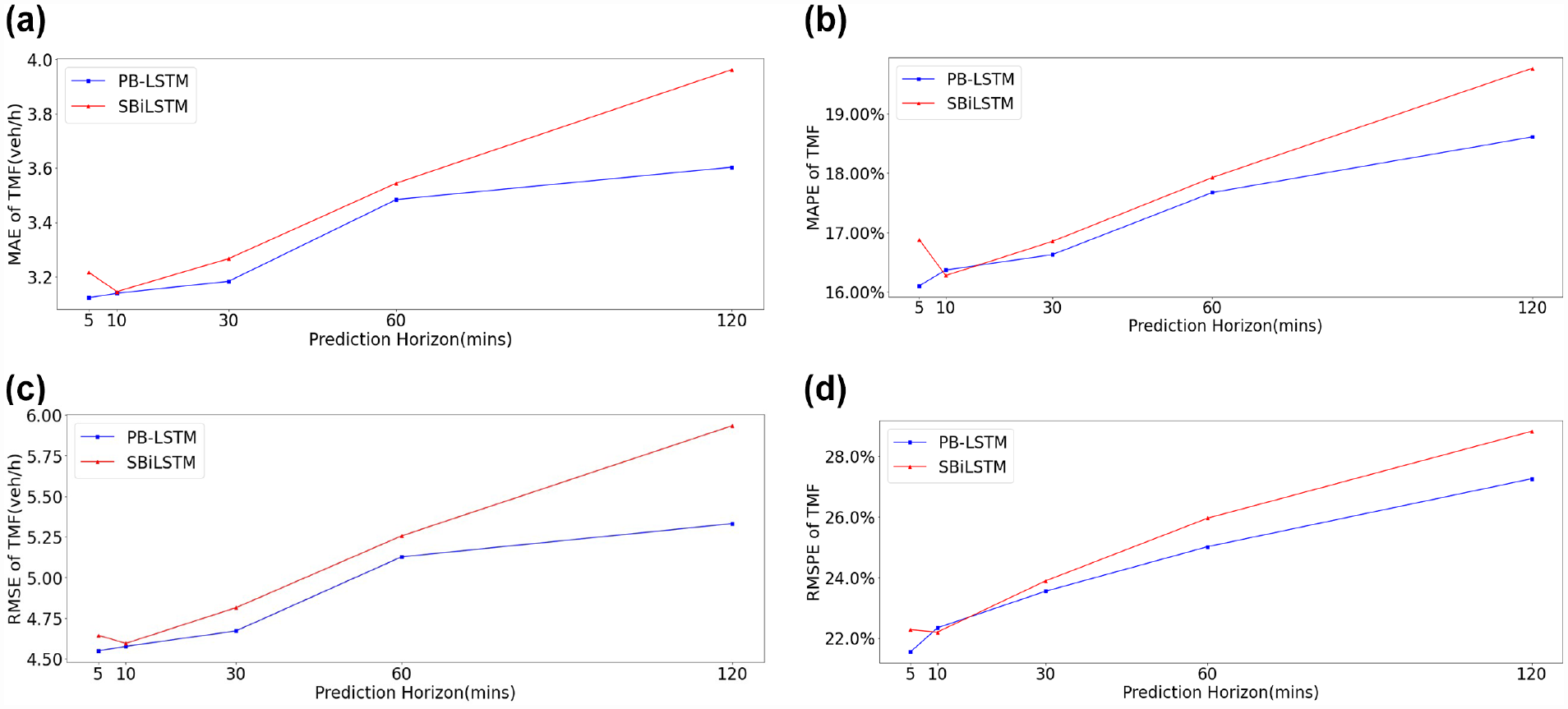
Weighted average performance comparison of two models for different prediction horizons when inputting 30 min historical traffic movement flows (TMFs): (a) mean absolute error, (b) mean absolute percent error, (c) root mean square error, (d) root mean square percent error.

Benefits of Location Clustering and Model Transferability

Because of the similarities in underlying travel demand and behavior, traffic flows may display similar time-varying patterns at several crossings in the same area. It is hypothesized that if clusters of intersections having similar attributes and traffic dynamics could be identified in advance and separate models could be constructed for each cluster, these models could provide better forecasts, especially when the models are applied to new locations (intersections in our case) where observations are not available to train the models. To test this hypothesis, the 20 intersections were classified into four groups using the well-known K-means algorithm ( 35 ) based on three different sets of intersection features, as shown in Table 4.

Table 4.

K-Means Classification Scenarios

Scenario	Input features
Scenario 1	Latitude	Longitude	Number of lanes for EW	Number of lanes for NS	Exclusive left lane for EW	Exclusive left lane for NS
Scenario 2	Daily TMFs for each approach
Scenario 3	Daily TMFs for each movement

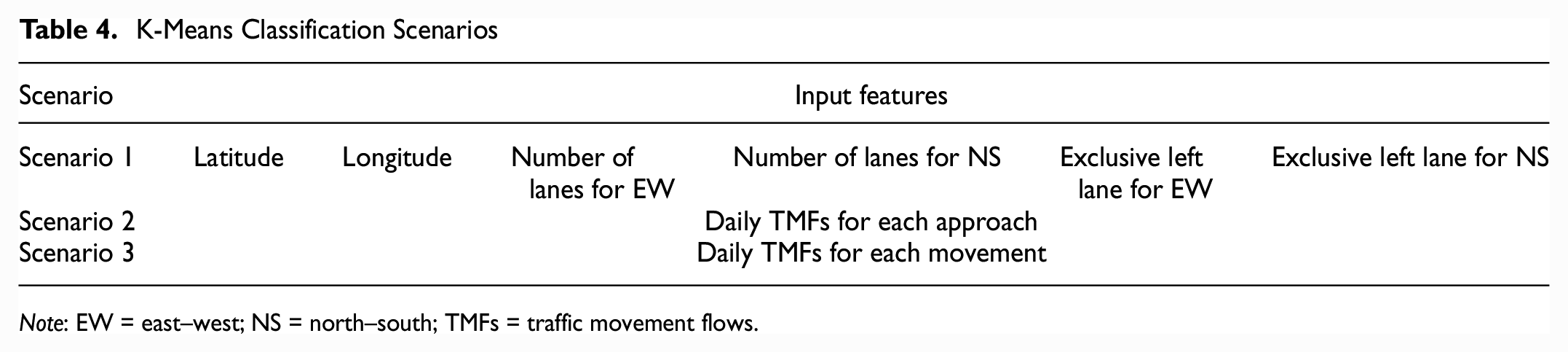
Note: EW = east–west; NS = north–south; TMFs = traffic movement flows.

Figure 13 shows the classification results under the three scenarios, whereas Figure 14 represents the impacts of the different traffic flow characteristics. Based on the obtained results, it is clear that the classifications under scenarios 2 and 3 are almost the same, indicating that the approach daily volume and the turning movement daily volume input deliver similar traffic variation patterns. Therefore, only scenarios 1 and 2 are considered in further analysis.

Figure 13.

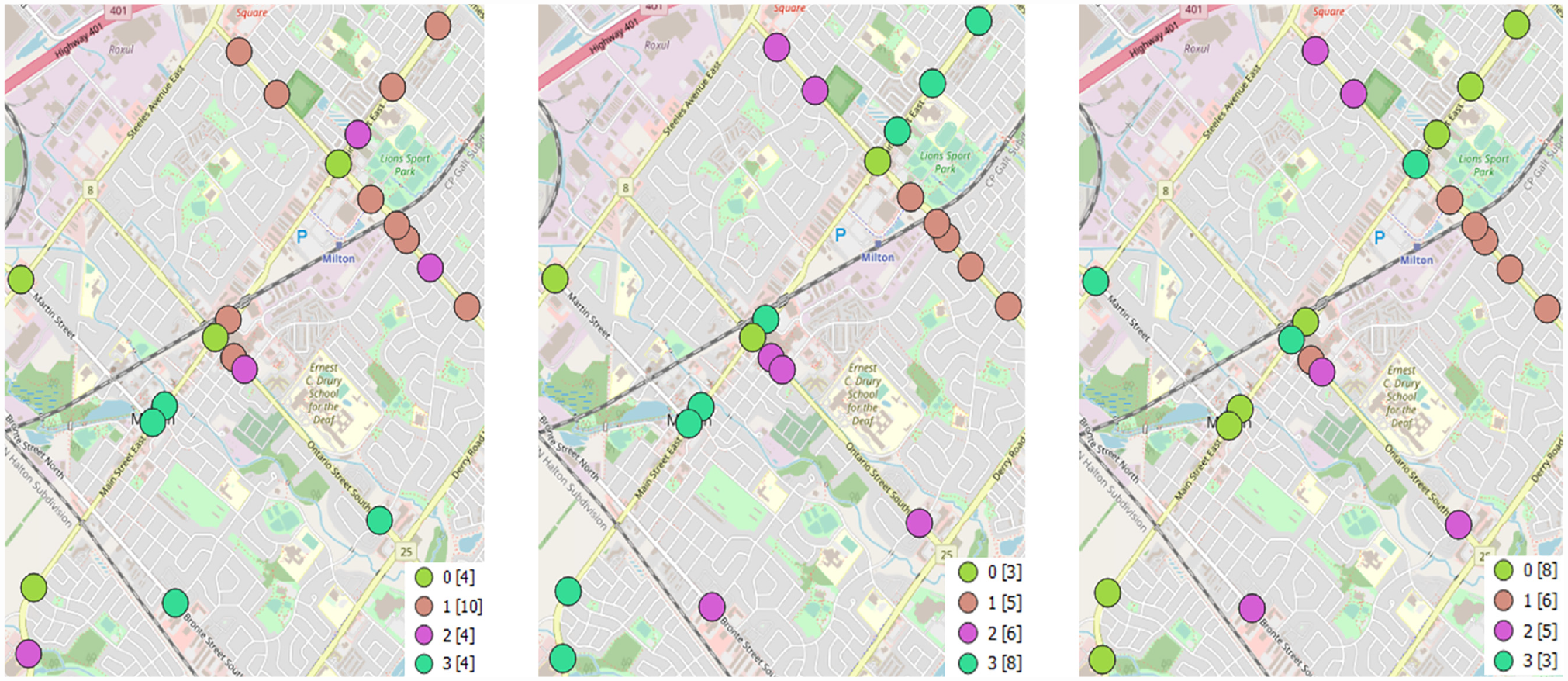
Classification results (scenario 1: left, scenario 2: middle, scenario 3: right).

Figure 14.

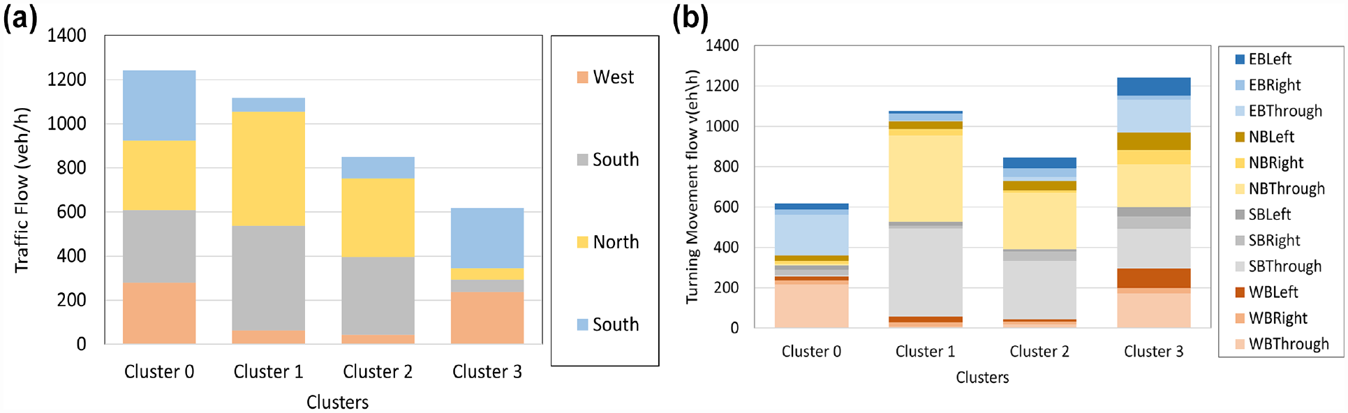
Characteristics of (a) scenario 2 and (b) scenario 3.

As a result, two distinct PB-LSTM models were created, PB-LSTM Geo (Scenario 1) and PB-LSTM App (Scenario 2), incorporating intersection cluster indications from the two clustering scenarios as an additional input. The base PB-LSTM is the one with no clustering but only intersection IDs, as denoted by the PB-LSTM ID. The input data range was set for 30 min and the forecasting horizon for 5 min.

The performance results are shown in Figure 15, where two observations can be made from these results. First, the two models, considering clustering, performed better than the one without considering clustering because the clustering label provided additional geographical or daily traffic flow information. Second, the performance superiority of the two models with different clustering scenarios is mixed with the non-consistent outcome at some intersections; therefore, the PB-LSTM Geo outperformed the PB-LSTM App while at others the opposite was true.

Figure 15.

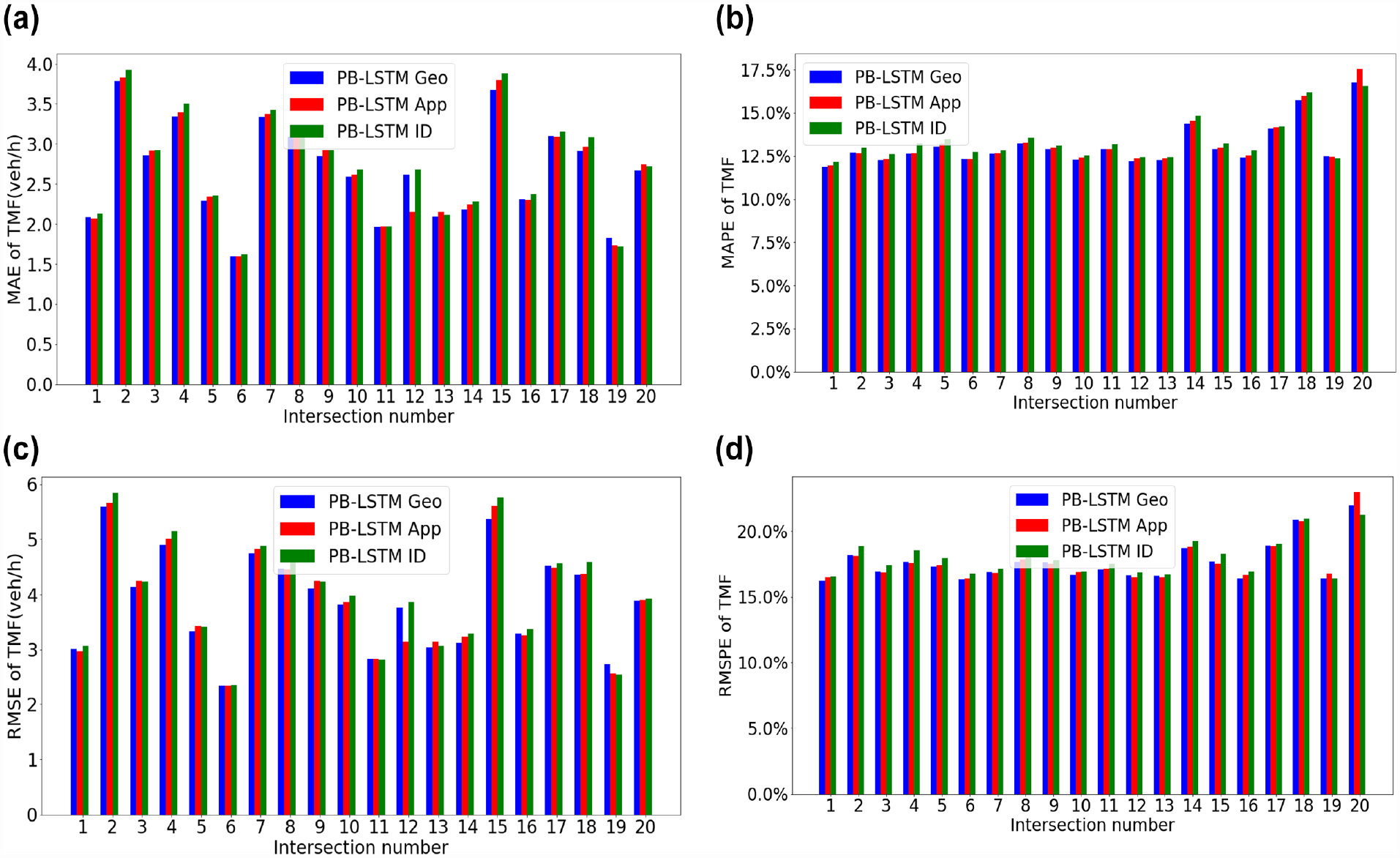
Comparison of PB-LSTM with the geometry classification label, PB-LSTM with approach classification label, PB-LSTM with the ID numbers, and typical LSTM models when being applied in 20 intersections: (a) mean absolute error, (b) mean absolute percent error, (c) root mean square error, (d) root mean square percent error.

One of the main reasons for including a clustering step is to improve the transferability of a forecasting model, that is, the ability of a model to forecast the flows at a completely new location or intersection. Therefore, the two trained models were applied to two completely new intersections, where data was not used in training the proposed model: the intersection of the Main Street and Leisure Centre Driveway (Geometry label: 2; Approach label: 2) and the intersection of Ontario Street South and Childs Drive (Geometry label: 3; Approach label: 2). The trained models were applied to generate one-step-ahead forecast of the turning movements at the test intersection. The cluster of the test intersection was determined according to each clustering method. For simplicity, this experiment considers only RMSE and RMSPE errors for evaluation. The input data range was fixed at 30 min. Moreover, the result for eastbound and northbound is shown in Figures 16 and 17, and other details are shown in Tables 5 and 6.

Figure 16.

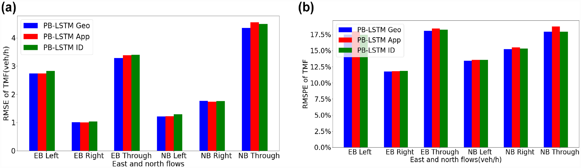
Comparison of PB-LSTM with geometry classification label, PB-LSTM with approach classification label, PB-LSTM with ID numbers, and typical LSTM models when applied in Ontario Street South and Childs Drive: (a) root mean square error, (b) root mean square percent error.

Figure 17.

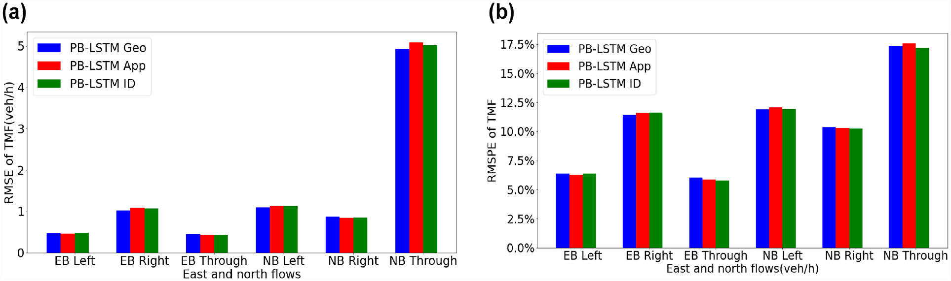
Comparison of PB-LSTM with geometry classification label, PB-LSTM with approach classification label, PB-LSTM with ID numbers, and normal LSTM models when applied to Main Street and Leisure Centre Driveway: (a) root mean square error, (b) root mean square percent error.

Table 5.

Model Comparison for Intersection of Main Street and Leisure Centre Driveway

		Eastbound			Northbound			Southbound			Westbound
Turning movements		Left	Right	Through	Left	Right	Through	Left	Right	Through	Left	Right	Through
Traffic volume		1,549,910	216,538	1,708,238	314,000	668,618	3,146,787	737,520	508,034	2,882,727	1,206,939	589,729	2,154,083
RMSE	PB-LSTM (Geo)	2.74	1.01	3.28	1.21	1.77	4.35	1.93	1.78	4.41	2.43	1.73	3.68
	PB-LSTM (App)	2.74	1.00	3.39	1.22	1.74	4.55	1.92	1.77	4.51	2.47	1.69	3.81
	PB-LSTM (ID)	2.82	1.03	3.40	1.29	1.75	4.49	1.96	1.93	4.53	2.49	1.70	3.78
RMSPE	PB-LSTM (Geo)	17.5%	11.8%	18.1%	13.4%	15.2%	17.9%	15.4%	16.2%	18.7%	15.8%	15.0%	17.8%
	PB-LSTM (App)	18.0%	11.8%	18.4%	13.6%	15.5%	18.7%	15.8%	16.9%	20.0%	16.3%	15.4%	18.4%
	PB-LSTM (ID)	17.5%	11.9%	18.3%	13.5%	15.3%	17.9%	15.7%	17.0%	19.0%	16.2%	15.3%	17.9%

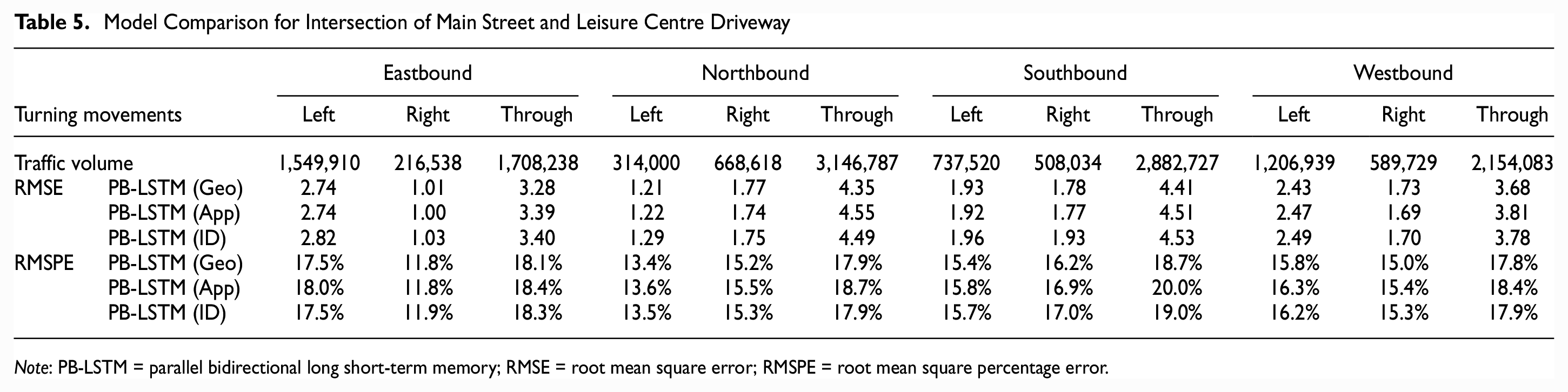
Note: PB-LSTM = parallel bidirectional long short-term memory; RMSE = root mean square error; RMSPE = root mean square percentage error.

Table 6.

Model Comparison for Intersection of Ontario Street South and Childs Drive

		Eastbound			Northbound			Southbound			Westbound
Turning movements		Left	Right	Through	Left	Right	Through	Left	Right	Through	Left	Right	Through
Traffic volume		297,751	585,761	288,633	534,409	641,840	4,575,455	277,812	320,201	4,573,341	607,004	324,450	360,887
RMSE	PB-LSTM (Geo)	0.474	1.022	0.450	1.100	0.876	4.916	0.971	0.570	5.765	0.748	1.019	0.558
	PB-LSTM (App)	0.462	1.085	0.432	1.132	0.847	5.084	0.941	0.590	5.909	0.715	1.034	0.544
	PB-LSTM (ID)	0.475	1.073	0.427	1.128	0.848	5.012	0.959	0.583	5.836	0.736	0.998	0.560
RMSPE	PB-LSTM (Geo)	6.4%	11.4%	6.0%	11.9%	10.4%	17.4%	11.2%	7.5%	18.5%	9.1%	11.5%	7.1%
	PB-LSTM (App)	6.3%	11.6%	5.9%	12.1%	10.3%	17.6%	11.2%	7.8%	18.8%	9.2%	11.7%	7.0%
	PB-LSTM (ID)	6.4%	11.6%	5.8%	11.9%	10.2%	17.2%	11.2%	7.6%	18.4%	9.1%	11.6%	7.1%

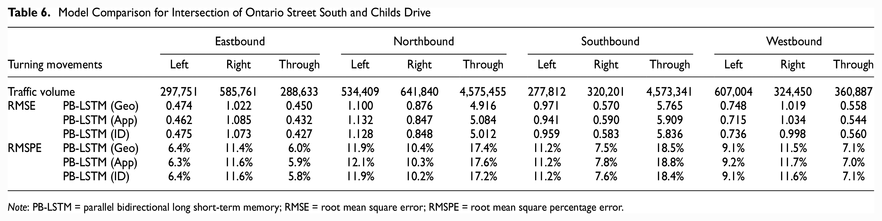
Note: PB-LSTM = parallel bidirectional long short-term memory; RMSE = root mean square error; RMSPE = root mean square percentage error.

To forecast the turning movements at the new intersections, the PB-LSTM Geo performed better for high traffic volume movements but not for low traffic movements. Regardless of the clustering step, the forecasting errors of the proposed models for the new intersections (data was not used in training the models) are comparable to those for the existing intersections (data was used in training the models).

Conclusion

Intersection traffic flow forecasting could provide valuable information for predicting traffic management and signal control as well as the timely provision of real-time information about road users. Recent advances in video-based real-time traffic monitoring solutions and ML have provided new opportunities for developing more reliable and accurate traffic forecasting models. Therefore, this research has explored the applications of several state-of-the-art DL models for short-term forecasting of intersection TMFs based on real-time TMCs. Specifically, a novel DNN model was proposed, which combines the latest LSTM model called stacked bidirectional LSTM with the traditional simple MLP, enabling learning of both short- and long-term time-varying patterns. Moreover, the performance of the proposed model was evaluated and compared with several state-of-the-art base models using two years of TMCs at 20 intersections in the city of Milton, Ontario, Canada. A series of experiments were also conducted to examine how the performance of the models was affected by several critical model settings, including the input data range, prediction horizon, and intersections clustering. The main findings and contributions of this research are summarized as follows:

• The proposed PB-LSTM model was shown to have a consistent performance advantage over several state-of-the-art time-series forecasting models, including SBiLSTM and MLP;

• Based on a sensitivity analysis of the effect of input data range on the model performance, the PB-LSTM model required input data as little as 30 min to achieve performance comparable with the SBiLSTM model using a data input range of 60 min;

• The performance of all models was shown to deteriorate by forecasting horizon; however, the proposed model had a much slower deterioration rate when compared with others;

• To improve the generalization ability of the proposed model, a clustering step was introduced to group intersections of similar attributes and use the grouping as an additional input to the model. Therefore, two clustering scenarios were proposed and their effect on the model performance was evaluated. As a result, it was found that the model with a consideration of clustering performed better than the one without clustering; however, the performance advantage was moderate at best.

This research could be extended in several directions. First, the idea of incorporating a clustering component in the overall forecasting model needs to be further explored, considering the relationship between the model generalizability and the intersection clustering methods. Second, the proposed model was found to be still limited in capturing abrupt short-term traffic variations. This could be attributed to either the learning capacity of the model or the inherent random variation of traffic. Moreover, as mentioned in Overall Performance section, the PB-LSTM underestimates TMFs during the peak hour where some separate models could be trained independently to solve the problem. Further research is therefore needed to explore other model forms (e.g., graph neural network) for capturing the network-wide interactions of traffic and examining the overall predictability issue of traffic. Finally, this work did not explore the question of how applicable the proposed model is to traffic in other cities. Therefore, applying it to other datasets, relevant to other cities, would be interesting to validate the obtained results.