Sage Journals: Discover world-class research

Abstract

Transverse joints are the weakest element of jointed pavements, and when these joints lack structural capacity, the onset of load-related distress is imminent. The most widespread measurement of the joints’ structural performance is the Load Transfer Efficiency Index (LTE), a ratio of the deflection of the two adjoining slabs. LTE can easily be assessed with a falling weight deflectometer, but this test procedure is not advisable for evaluation at the network level because of user safety concerns and because it can be excessively time-consuming. Traffic speed deflection devices like the traffic speed deflectometer (TSD) are suitable devices for network-level pavement structural evaluation. Yet, as of today, no interpretation technique to get structural health metrics for jointed pavements from TSD data has been published. In this paper, a backcalculation scheme based on slab theory is proposed to estimate the joints’ LTE from TSD deflection velocity measurements. The backcalculation problem formulation and its numerical solution using fast procedures are described in detail. The approach is tested with TSD data collected on the MnROAD test track. Overall, it was found that the backcalculation converges to reasonable estimates of the pavement structural properties and can furnish LTE estimates for most transverse joints from 5 cm-resolution TSD data, all at a reasonable computational cost. This allows for corridor-wide LTE assessment of a pavement’s joints using TSD measurements.

Keywords

jointed concrete pavement infrastructure condition assessment pavement structural testing and evaluation backcalculation TSD LTE index

Load Transfer Efficiency (LTE) for Structural Evaluation of Concrete Pavements

Proper maintenance of jointed pavements, like jointed (plain) Portland Cement concrete and composite pavements, requires knowledge of the present condition of both the pavement slabs and the load-carrying joints between slabs ( 1 – 4 ). Several backcalculation procedures exist for deriving the concrete’s and subgrade’s properties out of deflection measurements ( 5 ), whereas the performance of the load-carrying joints is assessed through the LTE test ( 5 – 7 ). LTE serves as an indicator of the joints’ structural health: joints with low values of LTE (weak joints) will eventually develop faults and induce slab spalling and loss-of-support-triggered fracture. Consequently, a tenet of jointed pavement preservation is preventing the loss of LTE ( 3 – 6 , 8 , 9 ).

The LTE test involves applying a load on a given slab close to its edge and measuring the deflection of the loaded slab and the adjacent unloaded one. The LTE of the joint between these two slabs is customarily defined in deflections ( 3 – 5 , 10 – 13 ):

LTE = \frac{w_{UL}}{w_{L}}

(1)

where W_UL and W_L are the deflections at the unloaded and loaded slabs, respectively. Alternative definitions and correction factors for LTE exist ( 1 , 4 , 5 , 9 , 10 ). However, the definition provided in equation 1 is the one most used ( 5 , 12 , 13 ).

LTE Testing Practice

The device of choice for assessing the LTE of in-service pavements is the Falling Weight Deflectometer (FWD), and standard testing procedures exist ( 5 , 7 , 13 ). The FWD excels at performing non-destructive evaluations of pavements at the project level, where few tests need to be made, and/or at locations closed to traffic, where the FWD can be operated safely. However, its use for network-level evaluations of in-service pavements is conditional on the test lanes being closed to traffic (thus disrupting the normal traffic flow) and exposes the FWD and its test crew to the possibility of being hit by an encroaching vehicle, which is an obvious safety concern ( 4 , 5 , 14 – 16 ).

Moreover, network-wide assessment of joints’ LTE with the FWD is impractical when considering the time required for testing: Testing a single joint for LTE takes roughly 5 min. At the usual 4.5 m (15 ft) joint spacing, the FWD would cover a stretch of pavement 60 m (180 ft) long (12 joints) per hour; an 8h shift may be enough to cover only about 1.1 lane-km (0.7 lane-miles) of pavement at the very most. Network-wide assessments at this rate are unfeasible because they would require too much time to complete ( 15 , 16 ).

Traffic Speed Deflection Devices (TSDDs), the Traffic Speed Deflectometer (TSD), and Deflection Testing on Concrete

TSDDs have been the subject of research since the 1990s. Such devices have been developed to overcome the limitations of stop-and-go and/or slow-moving deflection devices like the FWD and the deflectographs ( 14 – 16 ). By operating at traffic speed, TSDDs do not require lane closures to be operated safely. Furthermore, TSDDs collect dense data at intervals of 0.30 m (1 ft) or less ( 16 ). Reviews of TSDDs are available elsewhere ( 15 – 18 ).

The TSD, which is a specific TSDD, can survey 225–550 lane-km [140–350 lane-miles] a day ( 19 ). The TSD was first released in 2002 ( 14 ), and abundant literature has been published to date about its use at the network and project level and its comparison with other pavement deflection devices like the FWD or other TSDDs ( 15 – 21 ). Descriptions of the TSD are provided elsewhere ( 14 – 16 , 18 , 22 – 24 ), and in the Australian standards AG:AM/T017 and AG:AM/S006 ( 25 , 26 ), which refer to the device itself and the data collection process, respectively.

Since its early stages, the TSD has been regarded as capable of recognizing homogeneous sections and detecting weak spots within a pavement network for investigatory purposes ( 8 , 14 – 16 ). This makes it suitable for network-wide assessments of concrete pavements, in which low-LTE joints behave as localized weak spots ( 2 , 15 , 16 , 27 ). Scavone and colleagues presented an automated procedure for analyzing 1 m resolution TSD measurements from concrete and composite pavements ( 28 , 29 ). This analysis scheme simultaneously removes the random white noise in the TSD measurements and recovers the pulse response generated from structurally weak spots. As such, the weak spots may be localized within the pavement network, and thus further investigation with an FWD, and/or localized repair can be targeted.

In 2021, the fourth-generation TSD, with an upgraded sensing system capable of reliably reporting deflection velocity [v_y] measurements at a 5 cm resolution, was introduced in the United States. This TSD features ten Doppler sensors, located at −450, −300, −200, 130, 210, 300, 450, 600, 900, and 1500 mm from the center of the rear axle, plus the reference sensor located at 3500 mm. A trial run of the new TSD took place at the MnROAD test track (owned and operated by the Minnesota Department of Transportation) in September 2021, where both flexible and jointed rigid pavement segments were tested. In Scavone et al. ( 30 ), an in-depth analysis of the measurements at the jointed concrete sections within this testing site is presented: The analysis indicates that the 5 cm-resolution TSD measurements provide a clear depiction of the transverse joints’ responses. One key finding of this study is that on jointed pavements (or pavements with discontinuities of any type), the commonly assumed relationship between deflection velocity and deflection slope ( 31 ), reproduced as equation 2, is no longer valid.

S = \frac{v_{y}}{v_{x}}

(2)

In equation 2, v_y denotes the deflection velocity, S is the slope of the deflection bowl, and v_x is the TSD travel speed.

Instead, Scavone et al. ( 30 ) showed that the v_y measurements are constituted of two terms, one that relates to the slope of the deflection basin, plus an additional term that accounts for the changes in the shape of the deflection basin [w] after changes in the pavement structure such as layer thicknesses, material properties, or the presence of open cracks or joints. This term is mathematically noted as a partial derivative of the pavement deflection function w over time (equation 3).

S = \frac{v_{y}}{v_{x}} - \frac{1}{v_{x}} \frac{\partial w}{\partial t}

(3)

This partial derivative term becomes dominant on the v_y measurements collected near transverse joints. As such, TSD data interpretation must be done with v_y measurements instead of deflection slopes. Furthermore, it is shown that the linear-elastic jointed slab on a Pasternak foundation model ( 11 ) is adequate in describing the jointed pavement response to TSD loading. Therefore, the pavement properties, especially the joint LTE, can in principle be backcalculated from TSD v_y measurements using the slab on a Pasternak foundation model.

Research Objective

The objective of this paper is to backcalculate the LTE of a concrete joint from nearby deflection velocity measurements collected with a TSD. A backcalculation approach based on the slab-on-Pasternak foundation model ( 11 ) is implemented to solve for LTE. The ultimate intention is to provide a computationally fast and reasonably accurate tool for network-wide LTE estimation from a network-wide TSD data set.

Paper Organization

The remainder of this paper is divided into four sections: The Background section introduces succinctly the slab-on-Pasternak-foundation model. The Methods section elaborates on the formulation of the backcalculation procedure, and the approaches followed toward solving the variables of interest. The Validation section presents backcalculation results on real TSD data from a jointed pavement at the MnROAD test track and provides a comment on the results obtained. Finally, the Conclusions section is devoted to final thoughts on this methodology and opportunities for improvement and further research.

Background

A Brief Comment on the Slab-on-Pasternak-foundation Model

In the backcalculation approach presented here, the estimated v_y values to be matched to the TSD measurements are computed using a linear-elastic slab-on-Pasternak-foundation model ( 11 ). This model has been chosen because of its relative simplicity in material characterization and its smaller computational cost, as compared with finite-element models ( 3 , 32 ). Moreover, Deep et al. ( 3 ) pointed out that this model can reasonably simulate the rolling load of a heavy axle over jointed concrete, plus Scavone et al. ( 30 ) showed that it can simulate the TSD’s v_y measurements from jointed concrete pavements as well.

In the slab-on-Pasternak-foundation model ( 3 , 11 ), two infinite linear-elastic slabs that rest on a Pasternak subgrade (a combination of a Winkler foundation capable of resisting shear stresses as well) are linked by a single joint. One of the slabs is loaded, where the load consists of pressure p, where p is uniformly distributed over an area whose dimensions are 2a × 2b and whose center is located at a distance c from the joint. The slabs are characterized by their modulus of elasticity E, thickness h, and Poisson’s coefficient ν. The subgrade is characterized by its modulus of reaction k and shear strength modulus G (the Winkler foundation case corresponds to G = 0). The transverse joint is only characterized by its LTE index, as per equation 1. Figure 1 illustrates the variables involved in Van Cauwelaert’s model.

Figure 1.

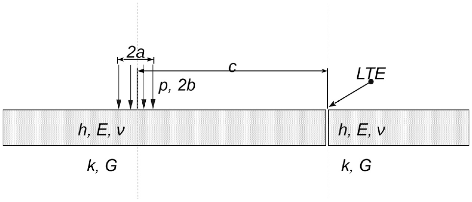
Linear-elastic slab-on-Pasternak-foundation deflection model. Variables involved.

The solution to the deflection basin for both slabs is the combination of the solution for an infinitely large slab plus a set of extra terms that account for the presence of the joint and the boundary conditions it imposes (ratio of deflections from both slabs equal to the LTE index, equality of shear stress on the subgrade under both slabs, and zero bending moment at the joint). The expressions for each of these terms are infinite integrals over a dummy variable and their formulation varies depending on the pavement structural properties’ values. These formulas are not reproduced in this paper so as not to overwhelm the reader, but they can be reviewed in Van Cauwelaert’s works ( 11 ).

Methods

Two Sequenced Optimization Problems to Solve the Pavement and Joint Properties

The backcalculation of materials’ properties and joints’ LTE from TSD measurements can be regarded as an optimization problem. The target variable to be minimized is the deflection matching error, the sum of squared errors (SSE) between the deflection measurements and a modeled response given a set of values for the parameters of interest ( 32 ).

Mathematically, such an optimization problem could be stated for TSD v_y data as well, assuming that the slab thickness h is known and ν can be reasonably set to a default value (ν = 0.20 for concrete [ 33 ]) (equation 4):

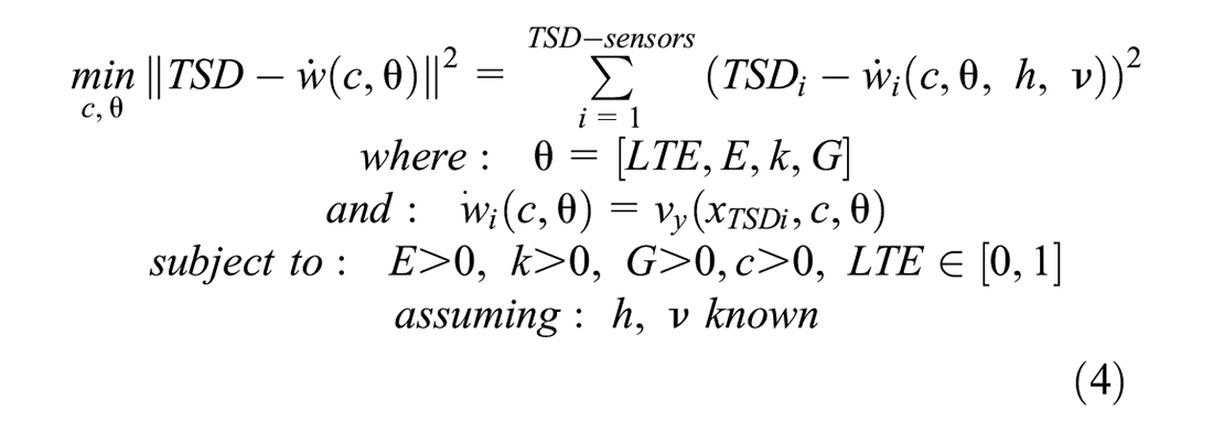
\begin{matrix} \min_{c, θ} ∥ TSD - \overset{\cdot}{w} (c, θ) ∥^{2} = \sum_{i = 1}^{TSD - sensors} {(TS D_{i} - {\overset{\cdot}{w}}_{i} (c, θ, h, ν))}^{2} \\ where : θ = [LTE, E, k, G] \\ and : \dot{w_{i}} (c, θ) = v_{y} (x_{TSDi}, c, θ) \\ subject to : E > 0, k > 0, G > 0, c > 0, LTE \in [0, 1] \\ assuming : h, ν known \end{matrix}

(4)

where TSD_i is the deflection velocity measurement collected by the TSD’s i-th sensor when the TSD wheel is at a distance c from the joint, and $\overset{\cdot}{W}$ _i(c, θ) is the fitted deflection velocity for a fixed point in the pavement surface computed from Van Cauwelaert’s model as a finite forward difference from two simulated deflection depths at different moments in time (equation 5):

\begin{matrix} \dot{w_{i}} (θ) & = v_{y} (x_{TS D_{i}}, c, θ) \\ = \frac{w (x_{TS D_{i}} - v_{x} Δ t, c - v_{x} Δ t, θ) - w (x_{TS D_{i}}, c, θ)}{Δ t} \end{matrix}

(5)

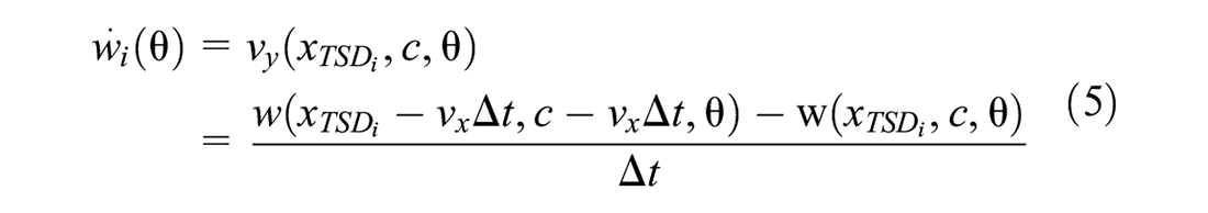
In equation 5, x_TSD-i represents the distance between the TSD’s i-th sensor and the TSD’s rear axle, and v_x is the TSD’s travel speed. Equation 5 accounts for that during the interval Δt, the TSD approached the joint by an amount equal to v_xΔt. But, in the slab-on-ground model, both the x-coordinate and the joint location are relative to the TSD wheel location; thus, one of the deflection estimates requires a correction, thus the x_TSD-i– v_xΔt and c – v_xΔt terms. The Δt can be chosen arbitrarily or can be set to match the TSD data resolution interval; for example, for 5 cm-resolution measurements, Δt = 5 cm/v_x.

Although conceptually simple, the formulation in equation 4 can be challenging to solve as it is a rather high-dimensional optimization problem (five unknowns) that may be tractable only if five or more valid v_y measurements were retrieved; otherwise, it may become ill-posed. Additionally, the formulation disregards measurements collected farther away from the joint, which could otherwise be mined to estimate the pavement’s material properties. Thus, we propose dividing the backcalculation scheme into two low-dimension problems to be solved in sequence, a procedure similar to Ullidtz’s ( 1 ) backcalculation from FWD data: a two-stage approach in which the concrete and subgrade properties are solved from mid-slab locations (using a simpler deflection basin model without the joint’s influence), reserving the measurements near the joint to solve for LTE. This second backcalculation problem assumes the results from the first problem as valid estimates of the slab and foundation strength parameters (Figure 2).

Figure 2.

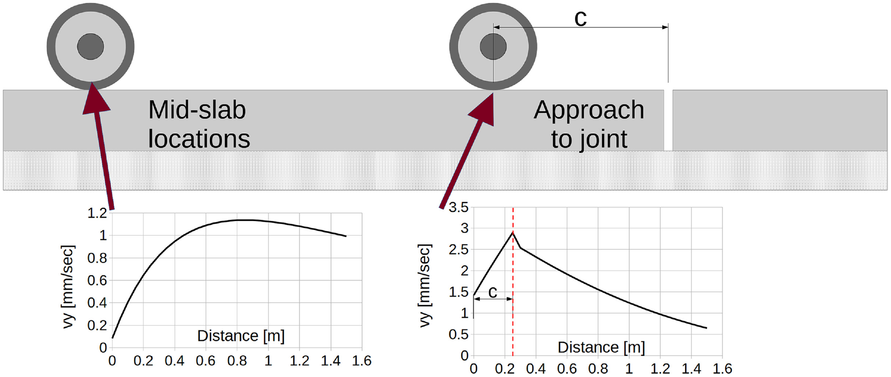
Concept representation of the two-profile backcalculation approach.

Mathematically, the first optimization problem is set to minimize the SSE for measurements collected away from the joint by varying the concrete pavement’s and subgrade’s strength parameters, namely E, k, G; the slab thickness h and the concrete’s ν are assumed as known. The fitted response, in this case, is the infinite slab component of Van Cauwelaert’s model, which is remarkably simplified compared with the full jointed slab model ( 11 ). The comparison TSD v_y data would be retrieved from measurements at a mid-slab location, named TSD_mid-slab. Thus, the optimization problem [OP1] to solve for k, E, and G is stated as equation 6:

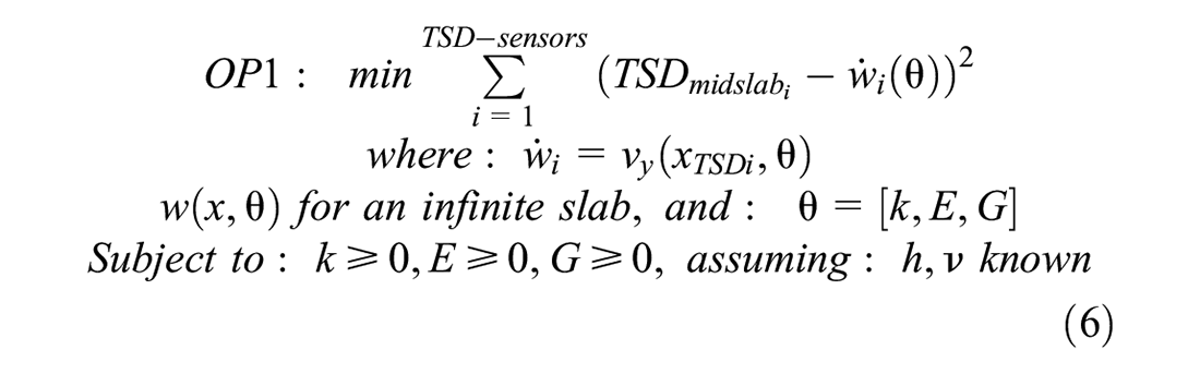
\begin{matrix} OP 1 : \min \sum_{i = 1}^{TSD - sensors} {(TS D_{midsla b_{i}} - {\overset{\cdot}{w}}_{i} (θ))}^{2} \\ where : {\overset{\cdot}{w}}_{i} = v_{y} (x_{TSDi}, θ) \\ w (x, θ) for an infinite slab, and : θ = [k, E, G] \\ Subject to : k \geq 0, E \geq 0, G \geq 0, assuming : h, ν known \end{matrix}

(6)

Additional restrictions can be added on k, E, and G for numerical stability purposes: These variables should not take unrealistically high values that transcend the usual range of values for engineering materials.

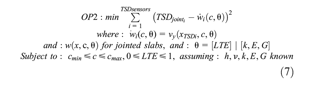
The second optimization problem [OP2] assumes that problem OP1 provides a good estimate of the pavement’s and foundation’s strength parameters and that those are valid near the transverse joint. Problem OP2’s objective function is the SSE between the TSD v_y measurements from all sensors collected near the joint (signal TSD_joint) and the full jointed-slab-on-ground model ( 11 ). The only decision variables are c and LTE. Under this formulation, the subgrade’s k-value at the joint location is assumed to be equal to the mid-slab value, and so it is assumed that no significant loss of support occurs under the joint. This formulation, however, has two main advantages:

The two decision variables are constrained. LTE cannot be negative or greater than 1. Similarly, c cannot be negative. Moreover, the pre-processing stage of the TSD measurements could provide hints about the exact location of the transverse joint: on 1 m data processed by Basis Pursuit Denoising ( 28 , 29 ), the joint is within 1 m from the station at which a pulse response was recovered. Meanwhile, on 5 cm data, the high-amplitude pulses on the v_y signal indicate the location of the joint within ± 5 cm ( 30 ). Thus, given the approximate joint location, narrow lower and upper bounds for c (c_min and c_max) can be defined for a given set of TSD v_y measurements.

Setting OP2 as a low-dimensional optimization problem simplifies computation, reduces the risk of the problem becoming ill-posed if few TSD sensors provide valid readings or are affected by measurement error, and allows for visual analysis of its numerical solver performance: The sub-optimal combinations of c and LTE can be plotted onto a 2-D grid to assess whether the solver implementation is converging or not.

Mathematically, problem OP2 is stated as:

\begin{matrix} OP 2 : \min \sum_{i = 1}^{TSDsensors} {(TS D_{join t_{i}} - {\overset{\cdot}{w}}_{i} (c, θ))}^{2} \\ where : {\dot{w}}_{i} (c, θ) = v_{y} (x_{TSDi}, c, θ) \\ and : w (x, c, θ) for jointed slabs, and : θ = [LTE] | [k, E, G] \\ Subject to : c_{\min} \leq c \leq c_{\max}, 0 \leq LTE \leq 1, assuming : h, ν, k, E, G known \end{matrix}

(7)

Numerical Solution of Problems OP1 and OP2

A numerical procedure based on gradient descent was implemented to iteratively seek a solution to problems OP1 and OP2. Conceptually, gradient descent aims at reaching a local minimum of a given function by proceeding down the direction with the steepest slope. If the given function is convex, which is often the case of squared errors, gradient descent would reach the global minimum ( 34 , 35 ).

The gradient descent implementation to solve problems OP1 and OP2 features a relaxed version of Hessian preconditioning, which accounts for the different orders of magnitude across the decision variables, as in the case for problem OP1, where the usual values for E (in metric units) are a hundred or thousand times the value of the subgrade’s k. Hessian preconditioning dynamically corrects the descent step size for each decision variable θ_i based on the curvature of the target function SSE, which is given by SSE’s inverse Hessian matrix. The relaxed Hessian preconditioning replaces the inverse Hessian matrix with a few second-order partial derivatives of SSE instead, thus saving computational cost ( 34 , 35 ).

Recalling θ is the vector containing the unknowns for problems OP1 and OP2, respectively, the iterative variable update (at iteration t) for the preconditioned descent is calculated as (equation 8):

θ (t + 1) = θ (t) - LR \times \frac{1}{Hjj} \times \nabla SSE (θ (t))

(8)

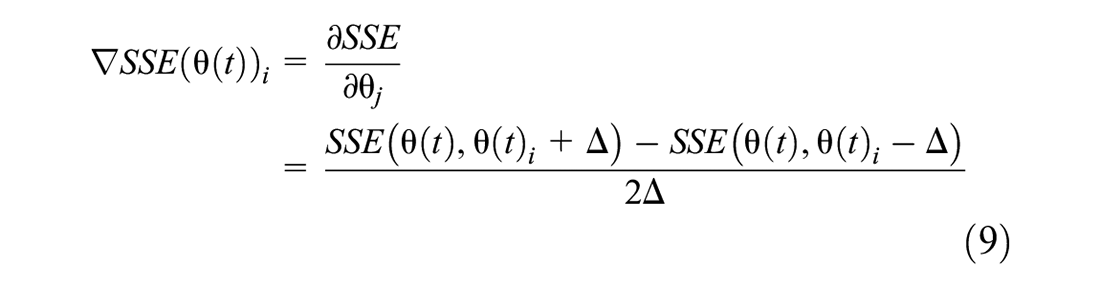
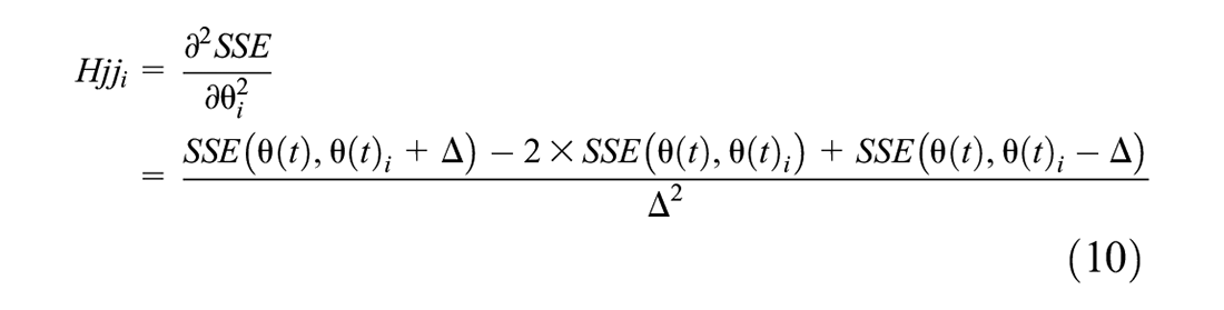
where SSE is the target function for problems OP1 or OP2 (equations 6 and 7), ∇SSE represents its gradient vector (equation 9), and 1/Hjj denotes a vector whose entries are the inverse of SSE’s second-order partial derivatives (equation 10). In equation 8, the product terms are element-wise products, not matrix product operations. The computation of the ∇SSE and the Hessian terms (Hjj) at each iteration is done coordinate-wise by calculating finite differences in SSE over increments in each coordinate θ_i (equations 9 and 10):

\begin{matrix} \nabla SSE {(θ (t))}_{i} & = \frac{\partial SSE}{\partial θ_{j}} \\ = \frac{SSE (θ (t), θ {(t)}_{i} + Δ) - SSE (θ (t), θ {(t)}_{i} - Δ)}{2 Δ} \end{matrix}

(9)

\begin{matrix} Hj j_{i} & = \frac{\partial^{2} SSE}{\partial θ_{i}^{2}} \\ = \frac{SSE (θ (t), θ {(t)}_{i} + Δ) - 2 \times SSE (θ (t), θ {(t)}_{i}) + SSE (θ (t), θ {(t)}_{i} - Δ)}{Δ^{2}} \end{matrix}

(10)

LR in equation 8 is the gradient descent learning rate, a hyper-parameter of the descent procedure that defines the step size down the SSE gradient, often set to a small quantity relative to the θ_i for numerical stability. Starting from any value for the vector θ(t = 0), gradient descent is repeated until θ(t) converges to a stable value: a local minimum of SSE. The descent failing to converge is often either because of implementation errors and/or an inappropriately large LR ( 34 ).

Figure 3 illustrates the numerical advantage of descent with Hessian preconditioning. Both examples shown correspond to a given simulated case study (the target values and departure values of the decision variables are the same in both examples). Without the Hessian preconditioning term, a value of LR that would let one decision variable descend would not change the value of the other decision variable. Meanwhile, once the preconditioning term is added to the descent, the iterative procedure converges smoothly.

Figure 3.

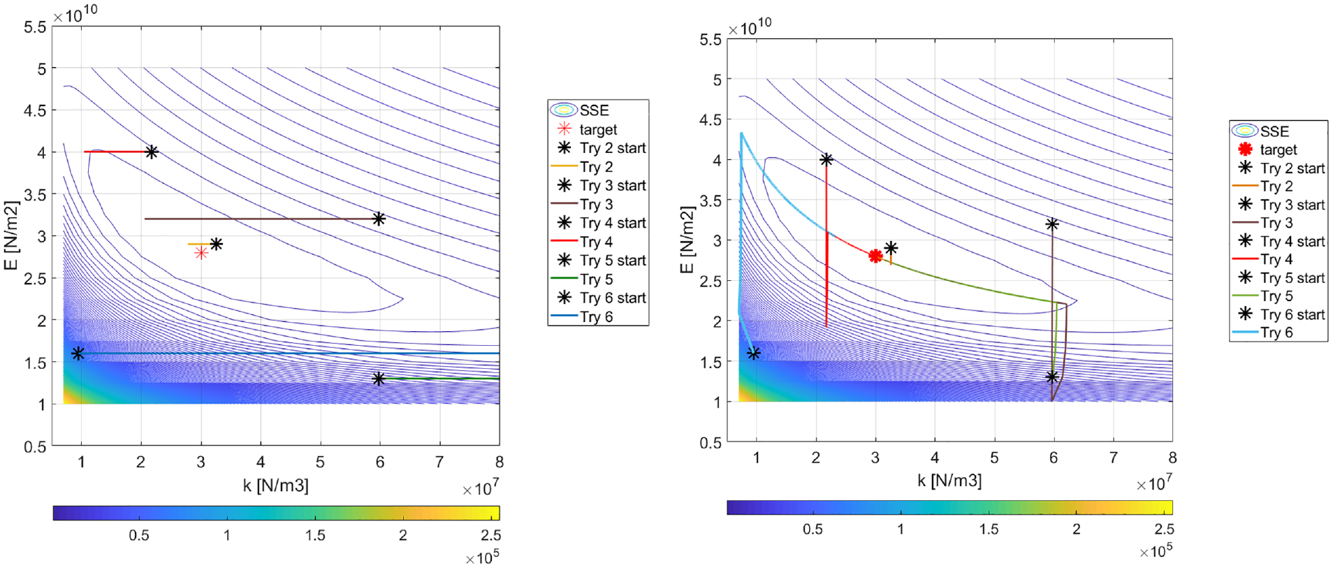
Effect of preconditioning in gradient descent. Left, descent without Hessian preconditioning (only one variable descends, LR = 1 × 10¹⁷). Right, descent with preconditioning (LR = 1 × 10⁻¹, both variables descend).

Problem OP1 Solver’s Implementation and Testing

Problem OP1’s solver was implemented with Hessian preconditioning and LR = 0.1, as this was found capable of minimizing the SSE out of v_y values in mm/s, and the decision variables in metric units (E and G in N/m², and k in N/m³). The backcalculation solver for OP1 was tested for a simulated case study (a unique set of target values for k, E, G) with five different start points. The simulated test was set as follows:

Concrete slab: E = 32000 MPa, ν = 0.20, h = 0.20 m

Foundation: Winkler material, k = 0.0326 MPa/mm, G = 0.

Load: 49 kN, pressure of 758 kPa [110 PSI], footprint dimensions [2a, 2b] = [0.14 m, 0.47 m].

Deflection velocity measurements were simulated for seven TSD sensors, located at 0.11, 0.21, 0.30, 0.45, 0.60, 0.90, and 1.50 m from the load center.

Figures 4 and 5 present the evolution of each decision variable and the trajectories followed over the SSE surface plot. The five test cases were solved in ¼ second on a personal computer running Matlab on a single CPU core; roughly 150–250 iterations were needed for the descent to get within 1% of the target k, E set, and 250–350 iterations were needed to get to 0.1%. This performance test shows that the solver for problem OP1 is robust and converges to its target accurately and quickly.

Figure 4.

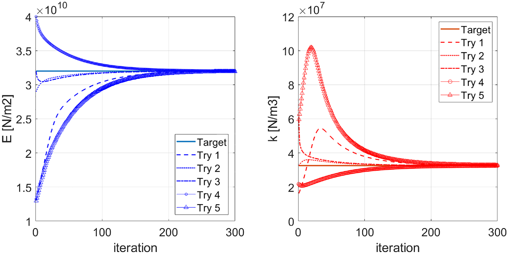
OP1’s solver performance test. Evolution of both decision variables during gradient descent. Left: evolution for E, right: evolution for the subgrade’s k.

Figure 5.

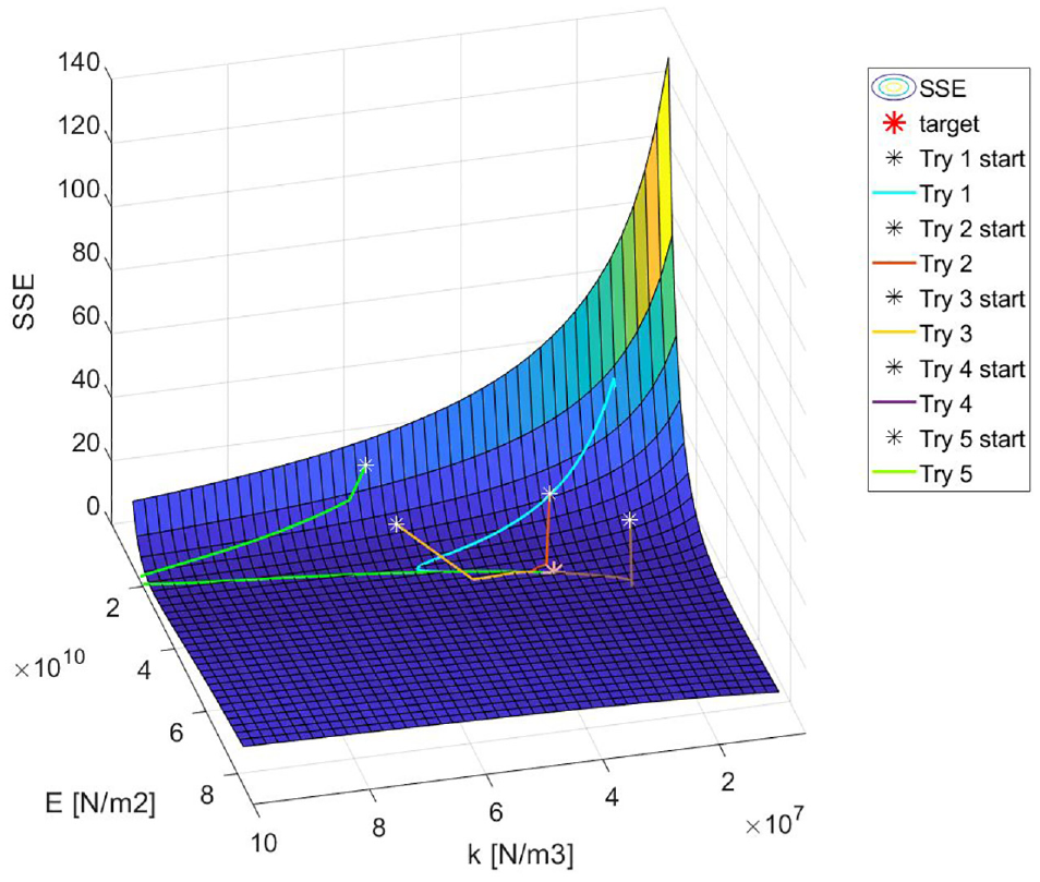
OP1-solver performance test. Descent trajectories for the backcalculated E and k during the gradient descent.

Problem OP2 Solver’s Implementation and Testing

A gradient-descent-based approach to solve OP2 was attempted unsuccessfully. During the implementation phase, the target function SSE was found to be non-convex: Bumps occur for any value of LTE when c equals any of the TSD sensor locations. These bumps are caused by the discontinuity at the joint, where the deflection slope component of v_y locally diverges. These bumps in the SSE function act as walls preventing gradient descent to reach the global minimum (Figure 6). Therefore, depending on the descent’s starting conditions, the descent might converge to the target or get stalled halfway. In the example shown in Figure 6, the targets are [c, LTE] = [0.40, 0.75].

Figure 6.

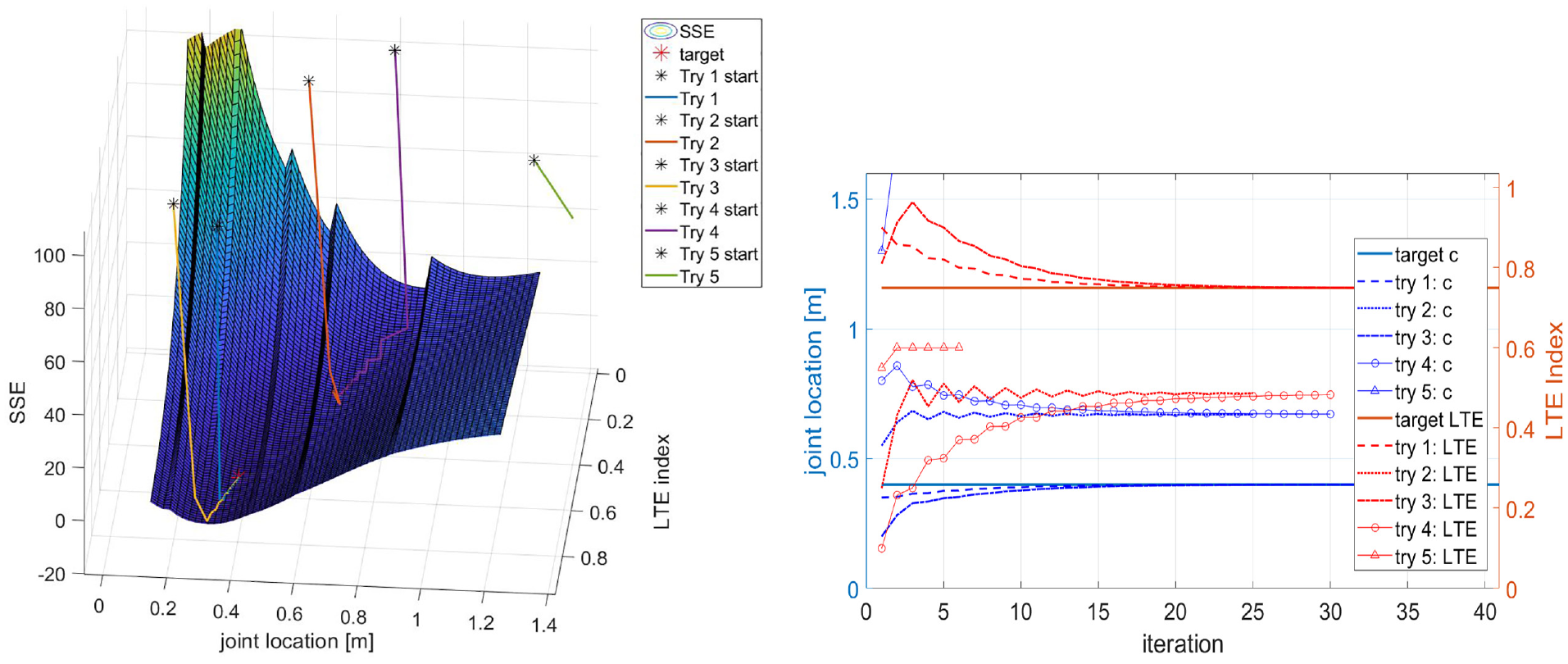
OP2’s solver performance test. Left: Evolution of both decision variables during gradient descent. Right: Descent trajectories for the backcalculated c and LTE during the gradient descent. Note how Try5 diverges from the target.

Thus, an alternative brute-force solution was implemented to solve problem OP2: SSE between calculated deflection velocities and the TSD measurements was computed for many combinations of c and LTE, and the combination that minimizes SSE was reported as the solution. This alternative solver takes advantage of the upper and lower constraints for the two decision variables.

Validation

Backcalculation of Joints’ LTE From Real TSD Measurements

This section presents a validation test of the entire backcalculation scheme over real TSD data from a jointed pavement segment. The TSD measurements were gathered at the MnROAD low-volume road in September 2021 during a demonstration run of the fourth-generation TSD.

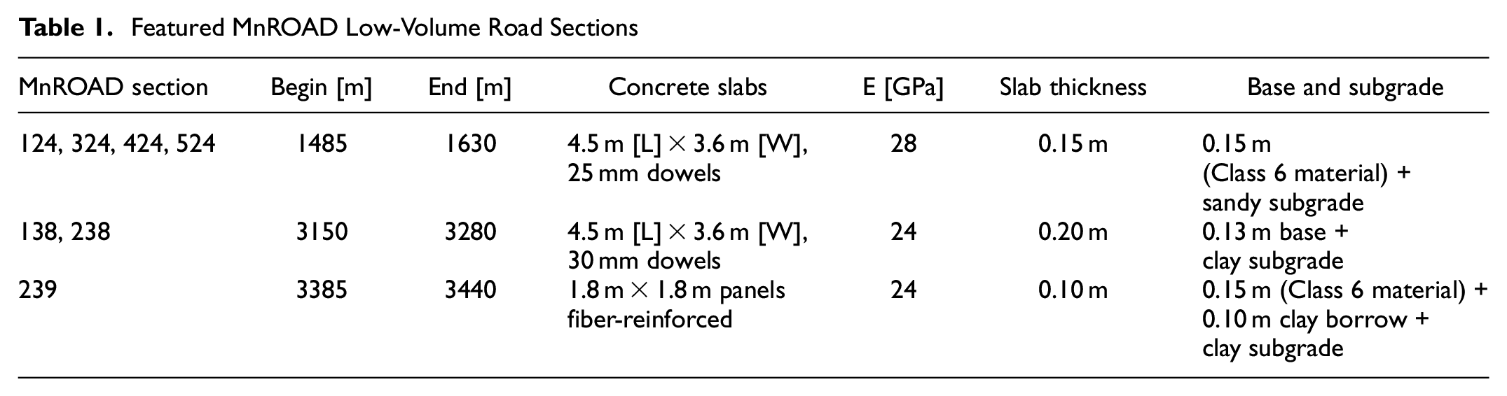
For this test, 5 cm-resolution data from three jointed concrete sections were made available by the TSD operator. Table 1 presents basic descriptive information about these segments, which were constructed in 2017 ( 36 – 38 ). Deflection testing with an FWD device was conducted in 2019 at several select transverse joints throughout these sections. The test results are publicly available through InfoPave ( 39 ), and LTE estimates were produced from these results following the guidelines in Schmalzer et al. ( 13 ).

Table 1.

Featured MnROAD Low-Volume Road Sections

MnROAD section	Begin [m]	End [m]	Concrete slabs	E [GPa]	Slab thickness	Base and subgrade
124, 324, 424, 524	1485	1630	4.5 m [L] × 3.6 m [W], 25 mm dowels	28	0.15 m	0.15 m (Class 6 material) + sandy subgrade
138, 238	3150	3280	4.5 m [L] × 3.6 m [W], 30 mm dowels	24	0.20 m	0.13 m base + clay subgrade
239	3385	3440	1.8 m × 1.8 m panels fiber-reinforced	24	0.10 m	0.15 m (Class 6 material) + 0.10 m clay borrow + clay subgrade

The backcalculation scheme for each section was implemented as follows:

As a pre-processing stage, the TSD deflection velocity data from all ten sensors were denoised by Haar wavelet denoising ( 40 ).

Then, each transverse joint was located in the data by identifying the stations at which high-amplitude peaks were recorded.

For each identified joint, the measurements gathered between 2.25 m and 1.75 m ahead of the joint station were utilized as mid-slab measurements to backcalculate k and E (problem OP1, equation 6). The subgrade was assumed a Winkler subgrade in this test. The average k, E estimates from all backcalculation attempts were kept as representative of that location.

Given OP1’s results, the measurements collected between 1.50 m and 0.20 m from the joint location were fed to OP2’s brute-force solver to estimate c and LTE. At each call to OP2’s solver, c was constrained to the difference in stations between the input measurement station and the joint location plus/minus 0.20 m.

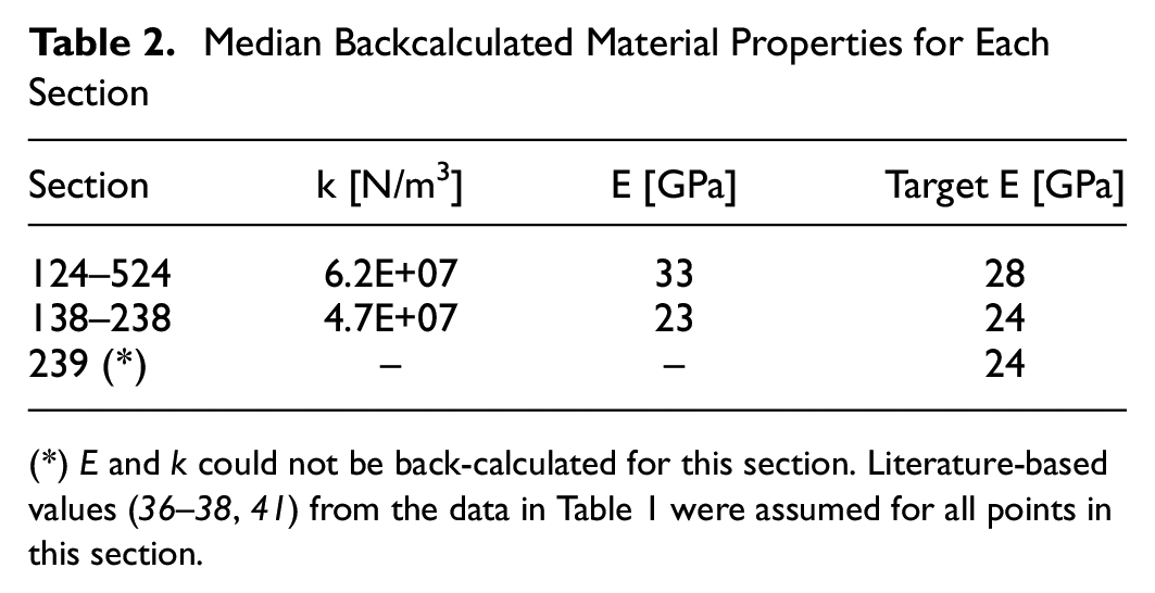
Step 3 could not be implemented for section 239; the pavement’s short slabs did not allow for the TSD to get a mid-slab measurement without any influence from the joint. Thus, for this section, default k and E values were assumed from literature ( 36 – 38 , 41 ) based on the available information (Table 1). Meanwhile, the median back-calculated k and E for sections 124-524 and 138-238 are shown in Table 2). The backcalculated LTE indices for all detected joints were plotted for easy visualization (Figures 7 –9), and the numerical results for those joints for which FWD-based LTE estimates exist are presented in Table 3. The computation time for each section was between 40 and 60 minutes.

Table 2.

Median Backcalculated Material Properties for Each Section

Section	k [N/m³]	E [GPa]	Target E [GPa]
124–524	6.2E+07	33	28
138–238	4.7E+07	23	24
239 (*)	–	–	24

(*) E and k could not be back-calculated for this section. Literature-based values ( 36 – 38 , 41 ) from the data in Table 1 were assumed for all points in this section.

Figure 7.

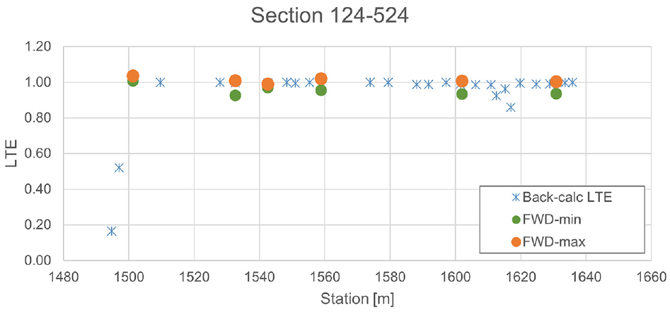
Backcalculated joints’ load transfer efficiency (LTE) for LVR section 124–524.

Figure 8.

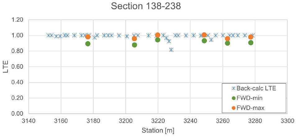
Backcalculated joints’ load transfer efficiency (LTE) for LVR section 138–238.

Figure 9.

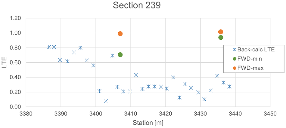
Backcalculated joints’ load transfer efficiency (LTE) for LVR section 239.

Table 3.

Joint LTE Backcalculation Results for Select Joints

Section	Station [m]	k [N/m³]	E [GPa]	LTE	FWD-based LTE
124–524	1,532.55	6.04E+07	33.7	1.00	0.93–1.00
124–524	1,542.55	6.95E+07	35.2	1.00	0.97–0.99
124–524	1,601.50	8.73E+07	32.4	0.99	0.93–1.00
124–524	1,628.90	1.10E+08	30.3	0.99	0.94–1.00
138–238	3,177.4	4.86E+07	24.5	1.00	0.89–0.98
138–238	3,205.15	5.43E+07	25.8	1.00	0.88–0.96
138–238	3,219.10	4.58E+07	24.0	0.99	0.94–1.00
138–238	3,246.50	4.50E+07	26.3	1.00	0.93–1.00
138–238	3,264.25	4.90E+07	22.7	1.00	0.90–0.96
138–238	3,278.45	3.77E+07	27.0	1.00	0.91–0.98
239	3,407.85	6.79E +07	24.0	0.21	0.71–0.99
239	3,434.8	6.79E+07	24.0	0.33	0.94–1.00

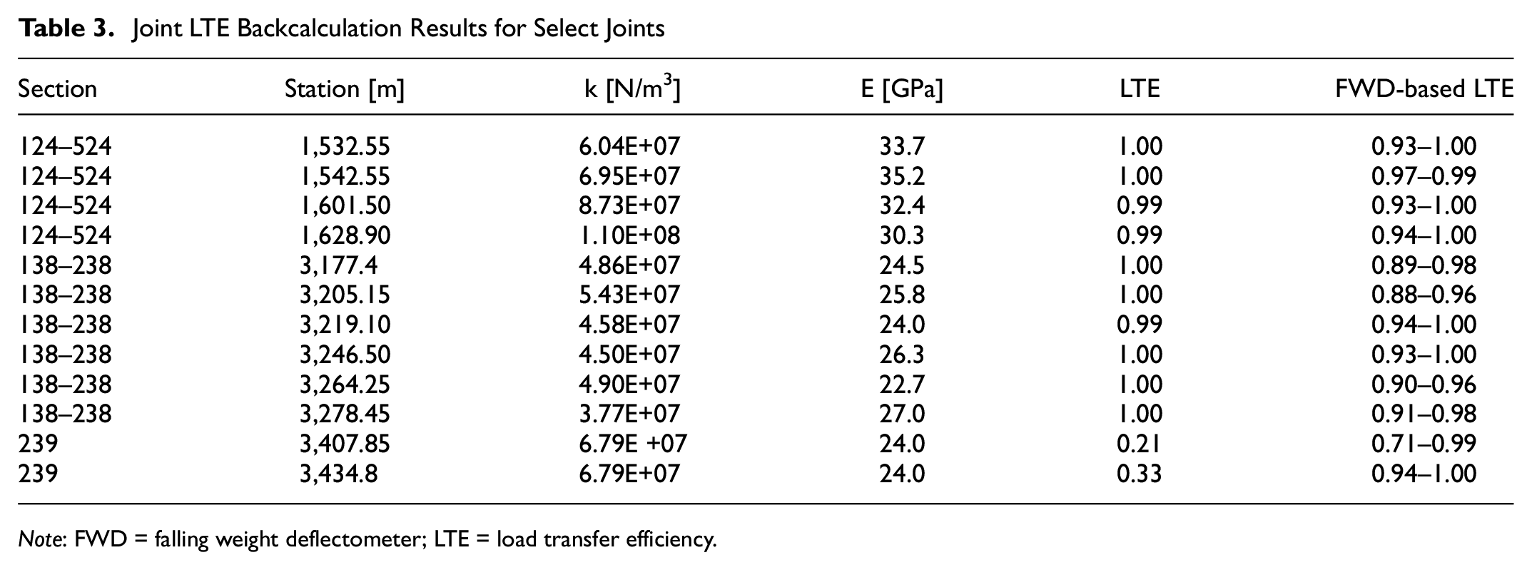
Note: FWD = falling weight deflectometer; LTE = load transfer efficiency.

Observing the station at which pulses were detected, it holds that a handful of the reported joints were false positives (either mid-slab cracks or misinterpreted events), as their distance to the previously reported event was less than the joint spacing. Moreover, some joints were missed by the automated detection, as their distance to the neighboring pulses was greater than the actual joint spacing. These missed joints are most likely in good structural health, having produced only a faint pulse response to the TSD load. These results encourage further research into creating an improved joint detection technique for 5 cm TSD data sets. In any case, the majority of the backcalculated events yielded reasonable results: the estimated material properties [k and E] fell within the usual range for concrete pavement on a granular sub-base (Table 2), and the LTE estimates for the joints for which FWD-based estimates existed were close to one another (except for section 239, which was known to deteriorate rapidly) ( 36 ).

Concerning backcalculated LTE indices, the estimates obtained roughly matched the FWD-based values, even observing that the comparison data were not collected simultaneously with the TSD survey (the FWD data are limited and 2 years older than the TSD survey), and the test track pavement may have deteriorated in the period between the two survey campaigns. Broadly speaking, the TSD reported that, overall, the pavement joints in sections 124–524 and 138–238 had good structural health, with the clear exception of the transition zone at one end of section 124–524, plus a single joint with an LTE lower than 0.85. Conversely, the TSD reported that section 239’s pavement (a thin 10 cm undowelled concrete structure) had highly deteriorated, as most of the transverse joints had poor LTE values (LTE lower than 0.70) ( 42 ). In any case, this paper’s backcalculation methodology fills in the missing information in the FWD-based LTE records with a single TSD sweep.

Conclusions

Scavone et al. ( 30 ) revisited the principle underlying TSD pavement deflection velocity measurements. The authors found that the TSD provides reliable deflection velocity measurements and that, for jointed pavements, these measurements may contain information about the transverse joints’ LTE index. The mechanistic backcalculation presented in this paper is the cornerstone of a comprehensive data analysis stream for TSD measurements for jointed concrete pavements, spanning both data denoising and interpretation. The data from the TSD trial run on the MnROAD test track proved that reasonable pavement properties and LTE estimates can be obtained. If adopted in practice, network-wide structural health checks for concrete pavements and their load-bearing joints could be performed swiftly with a TSD, obtaining valuable structural health metrics and saving days-long, expensive, and potentially unsafe survey campaigns with stop-and-go devices.

Opportunities for Further Research

Nielsen and Jensen recently stated ( 8 ) that information about the joints’ structural health might also be inferred from the v_y signals from the TSD’s sensors located at −130 and +110 mm from the rear axle wheel. This procedure is explained in detail in Nielsen et al. ( 43 ). A pairwise comparison between the LTE estimates from such a model and this paper’s backcalculation framework would be an interesting research exercise.

Finally, there is still room for enhancements to the backcalculation implementation to render it more comprehensive and/or realistic. Some examples follow:

A natural enhancement to the backcalculation core is the consideration of asphalt overlays. The implementation presented in this paper does not account for asphalt overlays on top of the concrete slab, yet Van Cauwelaert ( 11 ) provides the solution of the deflection bowl in both the concrete and asphalt overlay thicknesses and both materials’ elastic moduli. Thus, the implementation of this enhancement is worthwhile so that plain concrete and composite pavements can be assessed under the same framework.

Additionally, it may be of interest to also account for the subgrade’s loss of support of low-LTE joints. This phenomenon could be modeled as a drop in the subgrade’s strength parameters from the mid-slab values. Such an enhancement to the backcalculation problem is conceptually simple, yet it involves adding an extra variable to OP2’s brute-force solver, which entails additional computational costs.

The most time-consuming step in this backcalculation procedure is OP2’s brute-force search. Replacing this procedure with a less computationally demanding global optimization scheme is paramount for the eventual adoption of this LTE backcalculation within large-scale case studies. Alternatively, OP2 could be reformulated in a manner that it becomes a convex optimization problem that can be solved fast.

Also, an alternative approach to the two sequenced problems presented here may be warranted for short-slab pavements, in which the mid-slab measurements cannot be simulated with an infinite slab model. Thus, to avoid resorting to the high-dimensional backcalculation problem for jointed pavements (equation 4), a computationally fast and rational alternative interpretation technique for the TSD measurements must be sought.

Overall, this paper is just one more building block to a comprehensive jointed pavement management framework, turning deflection data into structural health information concerning the concrete slabs, the subgrade material, and the load-bearing transverse joints. Consequently, the pavement manager may now design and allocate maintenance resources more rationally to reach the ultimate objective of maintaining the jointed pavement network in a state of good repair.

Footnotes

Acknowledgements

The authors would like to thank Dr. P. Deep (U. Nottingham, UK), for guidance in the understanding of Van Cauwelaert’s jointed-slab-on-ground model, and Dr. B. Davids (U. Maine, USA) for furnishing a copy of the EverFE software, which was used to beta-test the code implementation of the linear-elastic slab-on-ground model. Also, thanks to J. Daleiden (ARBB Systems, USA) for providing the deflection data from the 4^th-gen TSD trial run at the MnROAD LVR facility.

Author Contributions

The authors confirm their contribution to the paper as follows: Study conception: M. Scavone; analysis and interpretation of results: M. Scavone; S. Katicha; draft manuscript preparation: M. Scavone; E. Amarh; study direction and management; G. Flintsch, S. Katicha. All authors reviewed the results and approved the final version of the manuscript.

Declaration of Conflicting Interests

The author(s) declared no potential conflicts of interest with respect to the research, authorship, and/or publication of this article.

Funding

The author(s) disclosed receipt of the following financial support for the research, authorship, and/or publication of this article: This research was funded by the Transportation Pooled Fund project TPF 5-385: “Pavement Structural Evaluation with Traffic Speed Deflection Devices (TSDDs),” supported by the Federal Highway Administration, U.S. Department of Transportation.

ORCID iDs

Martín Scavone

Samer W. Katicha

Gerardo W. Flintsch

Eugene Amarh

Data availability statement:

The Matlab source-code to the back-calculation technique presented in this paper is available through GitHub at: https://github.com/MartinScavone/concreteTSD. This source code is released AS-IS under the terms of the CC BY-SA 4.0 International. The terms of the license can be found in: . The MnROAD TSD data set presented in this paper can be furnished by the corresponding author(s) upon reasonable request.

References

Ullidtz

Pavement Analysis. Elsevier, Amsterdam, 1987.

Phares

B. M.

Ceylan

Souleyrette

Smadi

Gopalakrishnan

Development of a High Speed Rigid Pavement Analyzer–Phase I Feasibility and Need Study. Iowa State University, Ames, 2008.

Deep

Andersen

M. B.

Rasmussen

Marradi

Thom

N. H.

Lo Presti

Simulating Deflection of a Jointed Rigid Pavement under Rolling Wheel Deflectometer (RAPTOR) Loading. In Proceedings of the 9th International Conference on Maintenance and Rehabilitation of Pavements—Mairepav9 ( Raab

, ed.), Springer, Cham, 2020. pp. 859–870.

Deep

Continuous Structural Evaluation of Rigid Pavements (JCP). University of Nottingham, England, 2021.

Pierce

L. M.

Bruinsma

J. E.

Smith

K. D.

Wade

M. J.

Chatti

Vandenbossche

Using Falling Weight Deflectometer Data with Mechanistic-Empirical Design and Analysis, Volume III: Guidelines for Deflection Testing, Analysis, and Interpretation. Federal Highway Administration, Washington, DC, 2017.

Huang

Y. H.

Pavement Analysis and Design, 2nd ed. Pearson, London, 2004.

Alavi

LeCates

J. F.

Tavares

M. P.

Falling Weight Deflectometer Usage. Transportation Research Board, Washington, DC, 2008.

Nielsen

C. P.

Jensen

Traffic Speed Deflectometer Measurements at Copenhagen Airport. In Eleventh International Conference on the Bearing Capacity of Roads, Railways and Airfields ( Hoff

Mork

Saba

, eds.), CRC Press, London, 2021, pp. 458–465.

Wadkar

Mehta

Cleary

Guo

Musumeci

Zapata

Kettleson

Load-Transfer Efficiencies of Rigid Airfield Pavement Joints based on Stresses and Deflections. Journal of Materials in Civil Engineering, Vol. 23, No. 8, 2011, pp. 1171–1180.

10.

Ioannides

A. M.

Korovesis

G. T.

Analysis and Design of Doweled Slab-on-Grade Pavement Systems. Journal of Transportation Engineering, Vol. 118, No. 6, 1992, pp. 745–768.

11.

Van Cauwelaert

. Pavement Design and Evaluation. The Required Mathematics and Its Applications. Federation of the Belgian Cement Industry, Brussels, Belgium, 2003.

12.

Březina

Grošek

Janků

Measurement of Deflections and Determination of Jointed Plain Concrete Pavements Stiffness by Falling Weight Deflectometer. Procedia Engineering, Vol. 190, 2017, pp. 162–169.

13.

Schmalzer

P. N.

Rada

G. R.

Miller

J. S.

Falling Weight Deflectometer (FWD) Testing and Analysis Guidelines Volume I. Federal Highway Administration, Federal Lands Highway Division, Washington, DC, 2007.

14.

Hildebrand

Rasmussen

Development of a High Speed Deflectograph. Danish Road Institute, Roskilde, Denmark, 2002.

15.

Rada

G. R.

Nazarian

Visintine

B. A.

Siddharthan

R. V.

Thyagarajan

Pavement Structural Evaluation at the Network Level. Federal Highway Administration. Office of Infrastructure, McLean, VA, 2016.

16.

Flintsch

Katicha

Bryce

Ferne

Nell

Diefenderfer

Assessment of Continuous Pavement Deflection Measuring Technologies. The National Academies Press, Washington, DC, 2013.

17.

Arora

Tandon

Nazarian

Continuous Deflection Testing of Highways at Traffic Speeds. The University of Texas at El Paso, 2006.

18.

Katicha

S. W.

Flintsch

G. W.

Shrestha

Scavone

Overview of TSDD Technologies and Their Network- and Project-Level Applications. Transportation Pooled Fund [TPF] Project -5(385) Report, Virginia Tech Transportation Institute, Blacksburg, VA, 2021.

19.

Baltzer

Pratt

Weligamage

Adamsen

Hildebrand

Continuous Bearing Capacity Profile of 18,000 km Australian Road Network in Five Months. In 24th ARRB Conference, Melbourne, Victoria, Australia, 2010.

20.

Katicha

S. W.

Flintsch

G. W.

Ferne

Bryce

Limits of Agreement Method for Comparing TSD and FWD Measurements. International Journal of Pavement Engineering, Vol. 15, No. 6, 2014, pp. 532–541.

21.

Elseifi

M. A.

Zihan

Z. U.

Assessment of the Traffic Speed Deflectometer in Louisiana for Pavement Structural Evaluation. Louisiana Transportation Research Center, Baton Rouge, LA, 2018.

22.

Muller

W. B.

Roberts

Revised Approach to Assessing Traffic Speed Deflectometer Data and Field Validation of Deflection Bowl Predictions. International Journal of Pavement Engineering, Vol. 14, No. 4, 2013, pp. 388–402.

23.

Katicha

S. W.

Shrestha

Flintsch

G. W.

Diefenderfer

B. K.

Network Level Pavement Structural Testing With the Traffic Speed Deflectometer. Report No. VTRC 21-R4. Virginia Transportation Research Council (VTRC), Charlottesville, VA, 2020.

24.

Katicha

S. W.

Flintsch

G. W.

Shrestha

Thyagarajan

Demonstration of Network Level Pavement Structural Evaluation with Traffic Speed Deflectometer: Final report. Virginia Tech Transportation Institute, Blacksburg, VA, 2017.

25.

Austroads. Pavement Data Collection with a Traffic Speed Deflectometer (TSD) Device. Austroads, Sydney, NSW, Australia, 2016.

26.

Austroads. Specification for Pavement Deflection Measurement with a Traffic Speed Deflectometer (TSD) Device. Austroads, Sydney, NSW, Australia, 2016.

27.

Katicha

S. W.

Flintsch

Bryce

Ferne

Wavelet Denoising of TSD Deflection Slope Measurements for Improved Pavement Structural Evaluation. Computer-Aided Civil and Infrastructure Engineering, Vol. 29, No. 6, 2014, pp. 399–415.

28.

Scavone

Katicha

Flintsch

Identifying Weak Joints in Jointed Concrete and Composite Pavements from Traffic Speed Deflectometer Measurements by Basis Pursuit. Journal of Computing in Civil Engineering, Vol. 35, No. 2, 2021, p. 04020062.

29.

Scavone

Katicha

S. W.

Flintsch

G. W.

Diefenderfer

Reweighted L1 Minimization for Network-Wide Pavement Weak Spot Detection from Traffic Speed Deflectometer Measurements. Virginia Tech Transportation Institute, Blacksburg, VA, 2022.

30.

Scavone

Katicha

S. W.

Flintsch

G. W.

Amarh

On the TSD Deflection Velocity Measurements: A Revision to the Current State of the Art and Discussion Over its Applicability for Concrete Pavements Assessment. International Journal of Pavement Engineering, 2022. https://doi.org/10.1080/10298436.2022.2138881

31.

Krarup

Rasmussen

Aagaard

Hjorth

P. G.

Output From the Greenwood Traffic Speed Deflectometer. In 22nd ARRB Conference, Canberra, Australia, 2006.

32.

Rohde

G. T.

Smith

R. E.

Determining Depth to Apparent Stiff Layer from FWD Data. Texas Transportation Institute, The Texas A&M University System, College Station, 1991.

33.

NCHRP. Guide for Mechanistic-Empirical Design of New and Rehabilitated Pavement Structures. In Material Characterization for Inputs into AASHTO 2002 Guide of the 2004 Annual Conference of the Transportation Association of Canada Quebec City, Quebec, 2004.

34.

Zhang

Lipton

Z. C.

Smola

A. J.

Dive into Deep Learning. Cambridge University Press, 2021.

35.

Peyré

Mathematical Foundations of Data Sciences. 2020. https://mathematical-tours.github.io/book. Accessed May 15, 2023

36.

Barman

Roy

Tiwari

Burnham

T. R.

Performance Benefits of Fiber-Reinforced Thin Concrete Pavement and Overlays. Minnesota Department of Transportation, 2021.

37.

Van Deusen

D. A.

Burnham

T. R.

Dai

Geib

Hanson

Izevbekhai

B. I.

Johnson

Palek

Siekmeier

J. A.

Vrtis

M. C.

Report on 2017 MnROAD Construction Activities. Minnesota Department of Transportation Research Services & Library, 2018.

38.

Khazanovich

Kosar

Evaluation of Long-Term Impacts of Early Opening of Concrete Pavements. Department of Civil and Environmental Engineering University of Pittsburgh, Saint Paul, MN, 2021, p. 190.

39.

LTPP InfoPave . https://infopave.fhwa.dot.gov/. Accessed May 24, 2022.

40.

Katicha

S. W.

Locally Adaptive Averaging of TSD Data With a Local False Discovery Rate Control. Virginia Tech Transportation Institute, Blacksburg, VA, 2022.

41.

PCA. Thickness Design for Concrete Highway and Street Pavements. Portland Cement Association, Skokie, IL, 1984.

42.

“TxDOT”, T. D. o. T. Pavement Manual. Texas Department of Transportation, 2021.

43.

Nielsen

C. P.

Nahoujy

M. R.

Jansen

Measuring Joint Movement on Rigid Pavements Using the Traffic Speed Deflectometer. Journal of Transportation Engineering, Part B: Pavements, Vol. 149, No. 2, 2023, p. 04023002.

Estimating Load Transfer Efficiency for Jointed Pavements from TSD Deflection Velocity Measurements

Abstract

Keywords

Load Transfer Efficiency (LTE) for Structural Evaluation of Concrete Pavements

LTE Testing Practice

Traffic Speed Deflection Devices (TSDDs), the Traffic Speed Deflectometer (TSD), and Deflection Testing on Concrete

Research Objective

Paper Organization

Background

A Brief Comment on the Slab-on-Pasternak-foundation Model

Methods

Two Sequenced Optimization Problems to Solve the Pavement and Joint Properties

Numerical Solution of Problems OP1 and OP2

Problem OP1 Solver’s Implementation and Testing

Problem OP2 Solver’s Implementation and Testing

Validation

Backcalculation of Joints’ LTE From Real TSD Measurements

Conclusions

Opportunities for Further Research

Footnotes

Acknowledgements

Author Contributions

Declaration of Conflicting Interests

Funding

ORCID iDs

Data availability statement:

References