
Abstract
Network screening or crash hotspot identification is an essential task of all road safety improvement programs. The most common approach to network screening is to use statistical models to predict the expected risk at the locations of interest and then rank them accordingly. The predicted risk used for ranking is mostly in the form of point estimates, without any consideration of the inherent uncertainty with the estimates, which could lead to identifying a wrong list of crash hotspots. This study aims to fill this research gap by employing a frequentist approach to finding a joint confidence region of risk for ranking locations and identification of hotspots. A case study on three-legged minor approach stop-controlled intersections in Kitchener, Ontario, is conducted to illustrate the proposed approach. Crash risk is modeled using a combination of a hierarchical full Bayesian negative binomial model and a multinomial logit model, which are then used to estimate the 95% confidence interval of the expected risk. For each location, the confidence region of rankings is obtained on the basis of the expected risk estimates. The results show that considering uncertainty in the crash hotspot identification process can lead to varied ranking positions for each location. In fact, considering uncertainty, the true value of the estimated crash risk is unknown. By quantifying uncertainty, it can be concluded that the true value of the estimated risk follows a distribution with different probabilities. As a result, consideration of uncertainty in the road safety analysis may help to identify hotspots more accurately.
Keywords
Network screening is the first step of road safety management that can effectively help allocate limited resources to road safety improvement plans. Network screening typically begins with estimating the risk level of all locations of interest within the road network, followed by identifying the crash hotspots, also known in the literature as crash-prone, black-spot, or hazardous locations. Crash hotspots are commonly defined as places that have experienced more crashes than comparable locations during a specific time period because of local risk factors ( 1 ). According to the Highway Safety Manual (HSM), network screening has five major steps, namely, “establish focus,”“identify network and establish reference,”“select performance measures,”“select screening method,” and “screen and evaluate results.” To improve road safety by implementing appropriate countermeasures, it is necessary to prioritize locations with many crashes. Therefore, the final output of network screening is a list of ranked hotspots based on the estimated safety level, which are then to be further analyzed in the subsequent detailed engineering studies. The HSM proposes three methods for ranking hotspots: sliding window, simple ranking, and peak searching. While sliding window and peak searching are commonly used to rank road segments, simple ranking is preferred for ranking intersections.
Given the limited available budget for safety improvement, identifying an accurate list of crash hotspots is a crucial task for decision-makers. Typically, using statistical models to predict the expected risk at different locations is the most common approach in road safety analysis. However, uncertainty in the predictions is an inherent characteristic of statistical models. Thus, in some cases, this uncertainty can lead to false negatives (i.e., identifying hotspot sites as safe locations) or false positives (i.e., identifying safe sites as hotspot locations).
The main objective of this work is to provide a framework to consider uncertainty in ranking and identifying crash hotspots. Here, a two-step approach is developed. In the first step, a full Bayesian approach is adopted to estimate the confidence interval (CI) of the risk of a location. In the next step, the risk estimates are used to generate a joint confidence region for ranking the hotspot locations.
The rest of this paper is structured as follows: the following section summarizes a literature review of the hotspot identification and uncertainty quantification methods. A general framework for constructing a confidence region on ranking the hotspot locations is introduced in the methodology section. It is followed by a case study to show how the proposed methodology can be implemented. Then, the detailed findings are presented in the results and discussion section. Lastly, the recommendation for future studies is discussed in the conclusion section.
Literature Review
Safety performance functions (SPFs), developed by fitting a statistical distribution to historical crash data, are a common approach for evaluating road entities’ risk levels. The Poisson distribution is one of the most used probabilistic models in road safety studies. While the Poisson model is quite simple to apply, it cannot deal with the overdispersion often found in crash data. Therefore, several models have been developed to account for the overdispersion in crash data. The most often used model is the negative binomial (NB) employed by several researchers to model crash data ( 2 ).
The NB distribution is generally derived from the Poisson distribution by including a gamma-distributed error term in the Poisson parameter. However, some researchers argue that it is not necessary to suppose that the Poisson parameter must only follow the gamma distribution ( 3 ). Thus, researchers have explored a range of other Poisson parameter distributions, resulting in a variety of additional forms of mixed-Poisson regression models, such as Poisson–Weibull (PW) and Poisson–lognormal (PLN) models ( 4 ).
All of the aforementioned models are only focused on a point estimate of the predicted crash frequency (i.e., mean) at a specific location. While point estimates may be useful for prediction, owing to their simplicity, they do not provide information on the uncertainty in the predictions. In general, there are two main categories of uncertainty in statistics: aleatoric and epistemic ( 5 ). Aleatoric uncertainty (known as data uncertainty) arises from the data distribution’s stochastic nature. Conversely, epistemic uncertainty (known as knowledge or systematic uncertainty) happens because of the accuracy of a prediction model ( 6 ). According to Abdar et al. ( 6 ), uncertainty quantification is important in any prediction model that is used for critical decision-making. In this regard, few studies have tried to consider uncertainty in the predictions by developing CIs for estimates of road safety.
In a first effort, Wood ( 7 ) derived a prediction interval (PI) for the crash frequency at a new location (i.e., prediction response), as well as a CI for the expected crash frequency (i.e., Poisson mean) from the NB model. In another attempt, Ash et al. ( 8 ) followed the initial study of Wood ( 7 ) and derived formulas for PI and CI from different mixed-Poisson regression models, including the Poisson–inverse–Gaussian, Sichel, Poisson–lognormal, and Poisson–Weibull models.
Another approach to considering uncertainty in the crash prediction model is the quantile regression (QR) model, which originated from econometric studies. A few attempts have been made in road safety using the QR method. Qin et al. ( 9 ) identified Wisconsin’s top 5% riskiest intersections using a 95% QR model. In another study, using the equivalent property damage only (EPDO) technique for considering the crash cost of different severity levels, Washington et al. ( 10 ) developed a non-parametric QR model. They evaluated locations based on the output of the QR model and the observed EPDO.
The full Bayesian (FB) technique is another possible solution to quantifying uncertainty in statistical data analysis. The FB approach combines prior and posterior information, resulting in a fitted distribution that can provide the estimated crash frequency ( 11 ). Several researchers have used FB models for hotspot identification ( 12 – 14 ). For example, Aguero-Valverde and Jovanis ( 15 ) applied a FB approach by considering multivariate PLN models to identify hotspots through crash severity estimation, and concluded that the multivariate FB model performs well for hotspot identification. Miaou and Song ( 16 ) ranked locations by crash cost rate using Bayesian generalized linear mixed models considering multivariate spatial random effects; their study analyzed the frequency of the crashes by three different severity levels, including fatal, major injury, and minor injury at the county level.
Unobserved heterogeneity associated with crash data is one of the uncertainty sources of crash prediction models. To fully address this issue of heterogeneity, Heydari et al. ( 17 ) proposed a Bayesian non-parametric Dirichlet process mixture model and evaluated the performance of their approach through a comparison with various types of model, including NB, random effects, and traditional latent class models. In another study, by considering heterogeneity in the mean and variance of the crash data, Heydari et al. ( 18 ) developed a Bayesian heteroscedastic random parameter PLN model on the highway railway grade crossings crash data of eight major Canadian provinces. They showed the effectiveness of their model in comparison with several standard models of random effects and parameters.
The FB flexibility in explicitly describing hierarchical structures is another advantage. Owing to the data collecting and grouping processes, hierarchical patterns are prevalent in crash data. Recent research has shown that using a hierarchical modeling method may improve the accuracy of the fitted models on the crash data ( 16 ). Huang et al. ( 14 ) developed a hierarchical FB framework for road safety hotspot identification; they used two hierarchical FB PLN models to consider constant and serial temporal correlation. The hotspot identification in that study started with ranking locations with respect to their average crash count estimated through each model using 3 years of historical crash data. Then, the crash-prone locations were identified by defining a percentage threshold for the top-ranked locations (e.g., top 5%). The results indicate that hierarchical FB models significantly outperform the common empirical Bayesian technique, even when it comes to hotspot identification considering only temporal correlation.
So far, all the studies that used the FB approach for hotspot identification obtained the final predicted crash frequency by taking an average from all possible values corresponding to the fitted distribution. To the best of our knowledge, no study has considered uncertainty explicitly in ranking and prioritizing locations for safety improvement.
Several studies in statistics and economics have considered uncertainty in the ranking. In general, uncertainty in the ranking of a population can be evaluated through two main approaches: the Bayesian and the frequentist frameworks. In the Bayesian framework, the uncertainty in the ranking is evaluated by defining credible intervals for an estimator, and the rankings are then obtained using posterior probability ( 19 ). However, the frequentist method is based on constructing a CI to rank a population. Such CIs can be developed using either the bootstrap and other computational methods ( 20 ) or differences in means ( 21 ). Most studies reported in the literature use a frequentist approach to produce CIs for individual ranks. However, recently, some studies have focused on developing a joint confidence region by considering simultaneous CIs for individual ranks.
For example, the paper of Klein et al. ( 22 ) reports what is thought to be the first study on conducting a framework to create a joint confidence region for ranking of US states, based on the mean of travel time, using the Bonferroni-corrected CI method. In another study, Rising ( 23 ) followed the method of Klein et al. ( 22 ) in generating a joint confidence region; however, these authors used a partial order set to develop the CI for the rank of US states in relation to the mean of travel time. Their results show that their set estimator could produce a shorter range for the same confidence region.
Mogstad et al. ( 24 ) also conducted a similar analysis to that of Klein et al. ( 22 ) to construct confidence sets for the joint ranking of a population. The only difference in their research is that they exploited joint confidence sets for the differences in the estimator value of certain population pairs instead of constructing simultaneous confidence sets for all population entities. They also implemented their method in another study ( 25 ) to construct a 95% confidence region for the ranking of academic journals and universities around the world, based on considering uncertainty in the impact factor.
Methodology
The main objective of this study is to identify hotspots by considering the uncertainty for rankings. A two-step framework is proposed. In the first step, a 95% CI for the crash risk of each location is estimated. Based on the calculated CI, a confidence region (CR) for the ranking of each location is then calculated in the second step. In the following, the details of each step are discussed.
CI of Crash Risk at Each Location
A 95% CI for the risk value of a given site can be calculated by estimating the lower and upper limits of crash frequency by severity. By considering the social cost of each severity level, the CI for risk can be calculated as
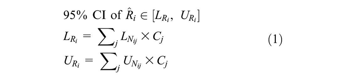
where
Then, a two-stage modeling approach is used to calculate crash frequencies for each severity level. First, we estimate the 95% CI for the total crash frequency (i.e., all severity levels) of a location using a hierarchical FB NB model. Accordingly, the crash frequency by severity at each site is derived by multiplying the probability of each severity type calculated by a multinomial logit model, as

where
FB Method for Predicting Crash Frequency (
FB analyses are characterized by their straightforward use of probability to quantify uncertainty in statistical data analysis. In FB analysis, statistical distributions are fitted to the model parameters, coefficients, and estimated crash frequency. The final predicted crash frequency can be obtained by taking an average or any quantiles from all possible values corresponding to the fitted distribution ( 11 ). This technique has three stages for calculating the predicted crash frequency at a specific traffic location ( 14 ).
Stage 1. Establishing a probability model for crash frequency:
In road safety, one of the most popular statistical models in use is the NB regression model, which is obtained from the Poisson model by assuming a gamma distribution for the error term (i.e.,
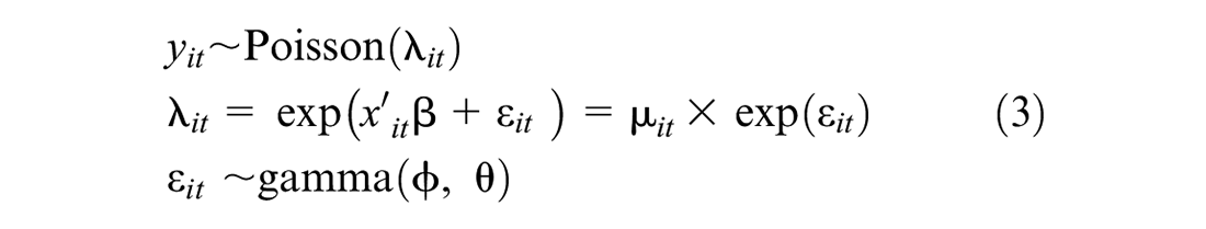
where
As can be seen in Equation 3, the error term changes across road locations and time. Therefore, the NB model can consider the overdispersion issue inherent in the standard Poisson model ( 2 ). However, the NB model limitation is that it does not account for the overdispersion associated with unobserved heterogeneities. Hierarchical models are an alternative to the usual statistical models used to address this issue. Therefore, in this study, a hierarchical NB (HNB) model is adopted to develop the FB model.
Stage 2. Assigning prior distributions to each model parameter:
The prior distributions are a measure of information about the effects of risk covariates and dispersion parameters on crash data. In the second stage, the parameters’ prior distributions must be specified to obtain the FB estimates. The prior distributions can generally be categorized into informative (i.e., prior information about the priors is available) and uninformative priors. Furthermore, in the context of a hierarchical FB model, it is assumed that a prior distribution assigned to a parameter has an error term depending on another parameter with a different distribution. With this definition, we follow the hierarchical Bayes structure presented by Miranda-Moreno et al. (
12
) for the error term (

where a and b are the fixed hyperparameter values, and the relation between the parameters is shown in Figure 1.
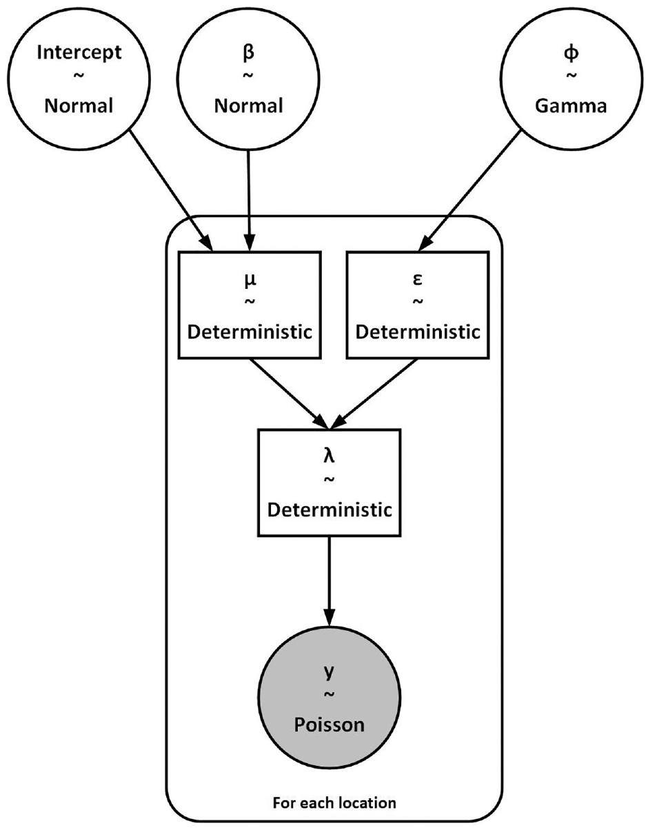
Hierarchical negative binomial model structure.
Stage 3. Calculating the proper posterior distribution for all unknowns’ coefficients:
Markov chain Monte Carlo (MCMC) sampling is a common method for establishing Bayesian inference through the random selection of parameter values from the fitted distribution and accuracy improvement by selecting new values, considering the posterior distribution ( 26 ). This method considers the prior distributions as an initial point and generates different chains of random points until the posterior distributions are converged using Bayesian theory. During the sampling, one part of the iterations will be considered burn-in, and the remaining ones will be used for parameter estimation.
Convergence is critical in FB models, since it will guarantee that a posterior has been found for the parameters. An assessment of convergence is made by examining the MCMC trace plots for the model parameters, as well as monitoring the ratio of Monte Carlo errors to standard deviations of the estimates; these ratios should be less than 0.05, as a general rule ( 27 ). In this study, the PyMC3 package is used in Python to generate the samples. After posterior calculations, the marginal distribution for the estimated number of crashes at a 95% CI will be obtained for each specific location.
Multinomial Logit Model for Predicting Crash Severity (
)
A collision severity model is used to predict the possible consequence of a collision. In this study, five possible discrete outcomes are considered: fatal, major injury, minor injury, minimal injury, or property damage only (PDO), each representing a specific level of severity. The probability associated with each severity type is modeled using a multinomial logit model. In a multinomial logit model, the probability that a collision results in a given severity type

where
The propensity value (Z) in Equation 5 is commonly expressed as a linear function of the site characteristics and attributes of the individual involved in the collision. The coefficients of the model will be calibrated using the maximum likelihood method.
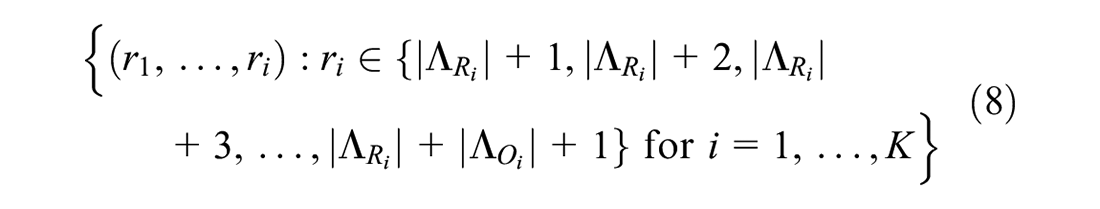
CR for Ranking of Hotspots
As a first step toward identifying hotspots, it is necessary to rank the locations based on their total risk. Generally, the estimated total risk is ranked using point estimates, such as the mean of the expected risk for each location (i.e.,
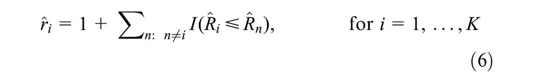
where
Once the CI has been calculated for each location,
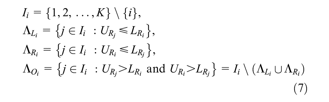
where, for each
1)
2)
3)
Based on these definitions, these three sets are mutually exclusive, and the number of elements in each set can be denoted by
Case Study
The application of the discussed methodology is demonstrated through a case study on the identification of high-risk three-legged stop-controlled intersections in Kitchener, Ontario, Canada. Three-legged stop-controlled intersections are the most common type of intersection in Kitchener, and they had the most crashes during the period of analysis. Therefore, the study focused exclusively on these intersections. This section discusses the details of data sources, risk modeling, and results of the analysis.
Data
A motor vehicle crash dataset (i.e., excluding pedestrian-involved crashes) for unsignalized intersections, consisting of 1,629 records of crashes that occurred from 2014 to 2018 in Kitchener, Ontario, Canada, was the primary source of data for this case study. Note that this study only considers crashes that occurred at intersections. Collisions that took place shortly before or after the intersections are not included in the analysis. Information related to each crash, such as crash date and time, location, driver and vehicle characteristics, severity level, and weather conditions, were included. The unsignalized intersection inventory data were obtained from the City of Kitchener’s data platform, from which data on all three-legged minor approach stop-controlled intersections (a total of 2,226 intersections) were extracted. In addition, the annual average daily traffic (AADT) for the intersecting roads for the period 2008 to 2020 was obtained from the City of Kitchener and the Open Data platform. Based on the analysis conducted by the City of Kitchener in their traffic and safety database management system (i.e., Traffic Engineering Software platform), an annual growth rate of 2% has been considered for the AADT. Therefore, for intersections with missing or incomplete AADT, the following approach was followed.
If a midblock had AADT for any year between 2008 and 2020, the AADT of the latest year was considered as a base of prediction for the other missing years, using a 2% annual growth rate, as calculated by the City of Kitchener.
Otherwise, the estimated data from the Open Data platform were considered as the AADT of 2014; the AADT of other years was predicted using the annual growth.
After following Steps 1 and 2, there were still 52 local street road segments (with two lanes) for which no observation or estimate was available in the City of Kitchener data platform. Thus, a rough estimate was considered, based on similar locations with available AADT. Therefore, for simplicity, the average of available estimated AADT from the Open Data platform for a local street with two lanes (i.e., an AADT of 500) was assumed for those few road segments without any available data.
To obtain the traffic volume on both major and minor approaches at intersections, first, the average AADT of 2014–2018 for the crossing streets of each intersection was integrated into the intersection inventory database. Then, to find the AADT of the minor and major streets, the road type of each crossing street was indexed from the midblock database, and the total AADT of the two major streets was considered as the AADT of the major approach. In the same way, the AADT of each minor direction was found. In some cases, the road type of all the connected segments was the same (e.g., all the crossing streets were major or minor types). In these cases, the sum of the two first highest AADT values was considered the major AADT, and the remaining AADT was considered the minor. Table 1 presents a brief statistical description of motor vehicle crash data by severity and traffic volume for all types of unsignalized intersection within the database.
Descriptive Summary of Motor Vehicle Crashes by Severity and Traffic Volume
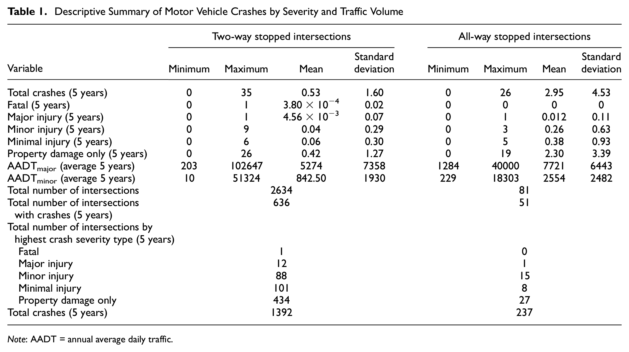
Note: AADT = annual average daily traffic.
Results and Discussions
Crash Frequency Model
Owing to a lack of full information about the various characteristics of the intersections, the traffic-exposure-only functional form was used to predict the mean of crashes through a hierarchal FB NB model:

where
For model calibration, Heydari et al. (
29
) and Miranda-Moreno et al. (
13
) showed that using an informative prior distribution for the dispersion parameter can result in a more accurate posterior. Therefore, the NB model was first calibrated using the maximum likelihood method, which resulted in a dispersion parameter of

Once the prior distributions were defined, the posterior distributions were calculated through the MCMC sampling method using the PyMC3 package in Python. For each parameter, four different chains consisting of 3,000 simulations were considered; the first 2,000 samples were used as burn-in iterations. Having tested various MCMC algorithms, such as Metropolis–Hastings, Gibbs sampler, Hamiltonian Monte Carlo, and no U-turn sampler (NUTS), we found that NUTS performed better on our model. As shown in Figure 2, the MCMC model converged on all parameters; this demonstrates the accuracy of the model.
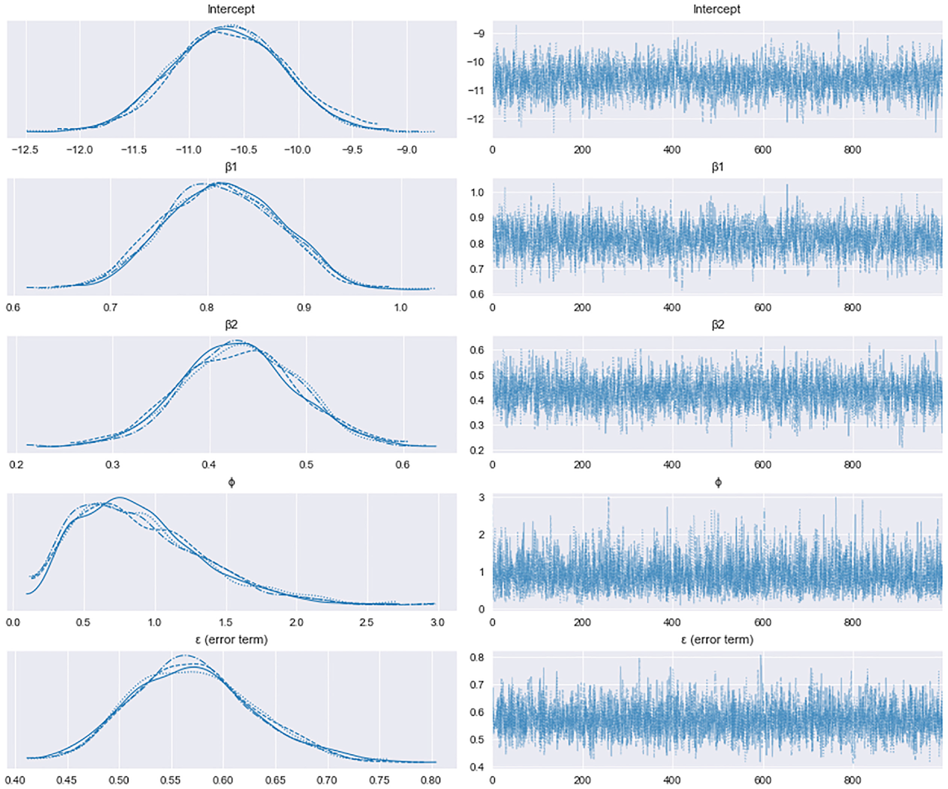
Trace plot of Markov chain Monte Carlo model for each parameter.
As a result, the expected posterior values of all parameters were obtained in the 95% CI. Table 2 shows that none of the regression coefficients contained 0 in their 95% CIs; this implies that all parameters were statistically significant in the model. Additionally, the results indicate that the ratio of Monte Carlo standard error (MCSE) to standard deviation (SD) of the estimates for all parameters was less than 0.05; this confirms the convergence of posterior distributions.
Summary of Model Calibration Results
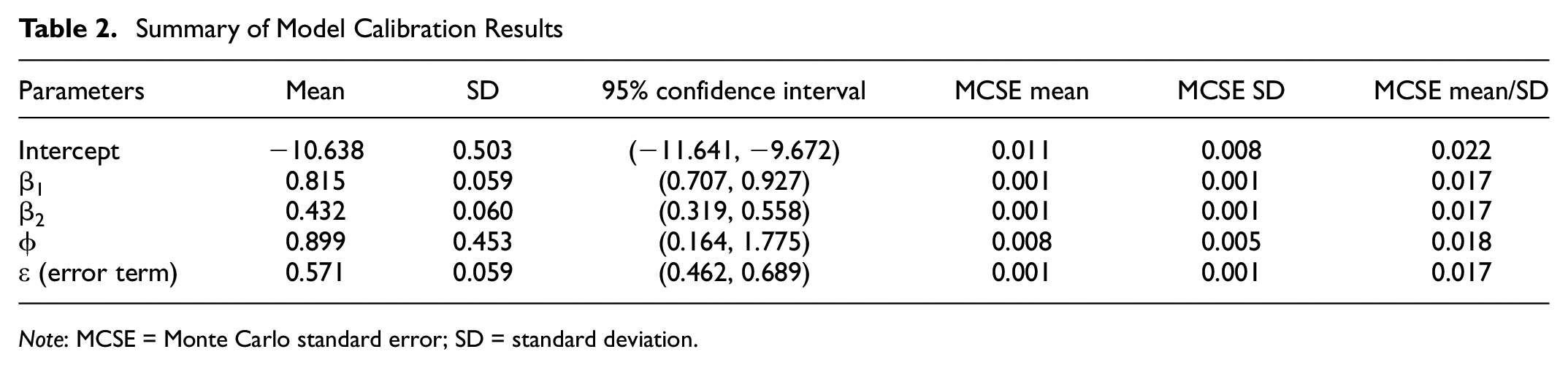
Note: MCSE = Monte Carlo standard error; SD = standard deviation.
Crash Severity Model
In this study, the crash database contained information about the number of fatalities, major injuries, minor injuries, and minimal injuries, if any, for each crash that occurred at a given intersection. However, owing to the low number of fatal motor vehicle crashes (i.e., only one fatality), it was difficult to develop a separate severity model for fatalities. As a result, the crash severities were classified into four levels:
fatality or major injury: if at least a person died or had a major injury; otherwise
minor injury: if at least a person had a minor injury; otherwise
minimal injury: if at least a person had a minimal injury; otherwise
no injury, i.e., PDO.
Based on this classification, each crash was categorized based on the highest level of severity with which it was associated. For example, if a crash resulted in a fatality, minor injuries, and PDO, this crash was labeled as a fatality or major injury, that being the highest level of severity.
To incorporate site-specific characteristics, the crash dataset was combined with the intersection inventory database. Table 3 presents a summary of the final dataset. Out of 1,629 motor vehicle crashes at unsignalized intersections during 2014–2018, there were 14 fatalities or major injuries (1 fatality and 13 major injuries), 133 minor injuries, 193 minimal injuries, and 1,289 cases of PDO.
Summary of Crash Database Variables
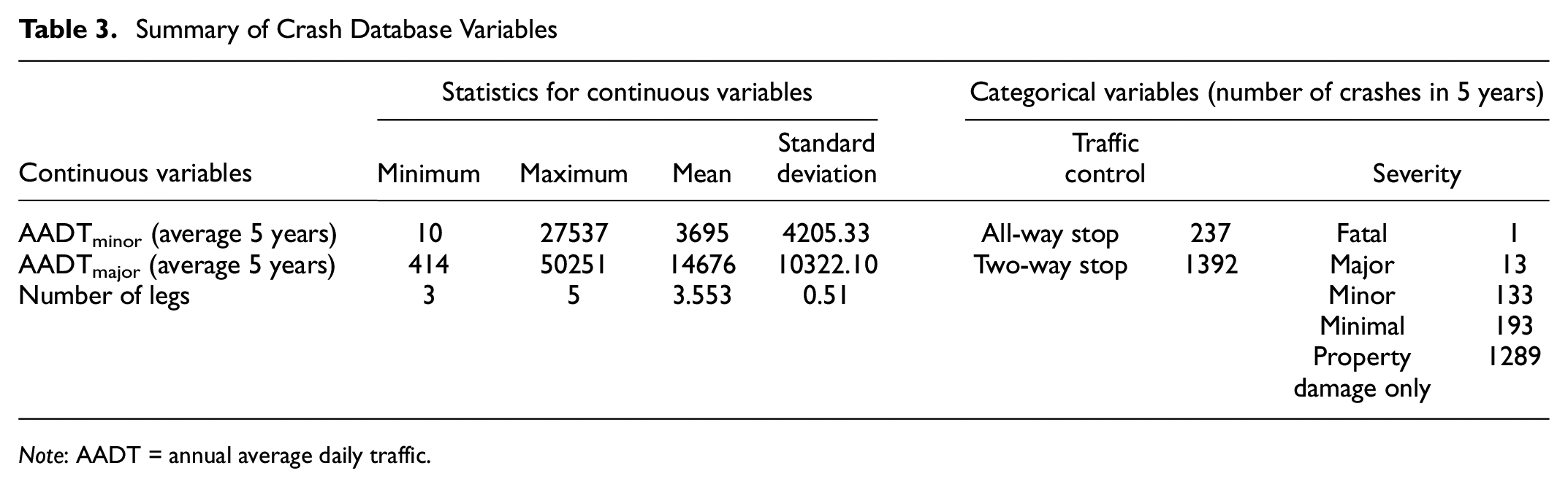
Note: AADT = annual average daily traffic.
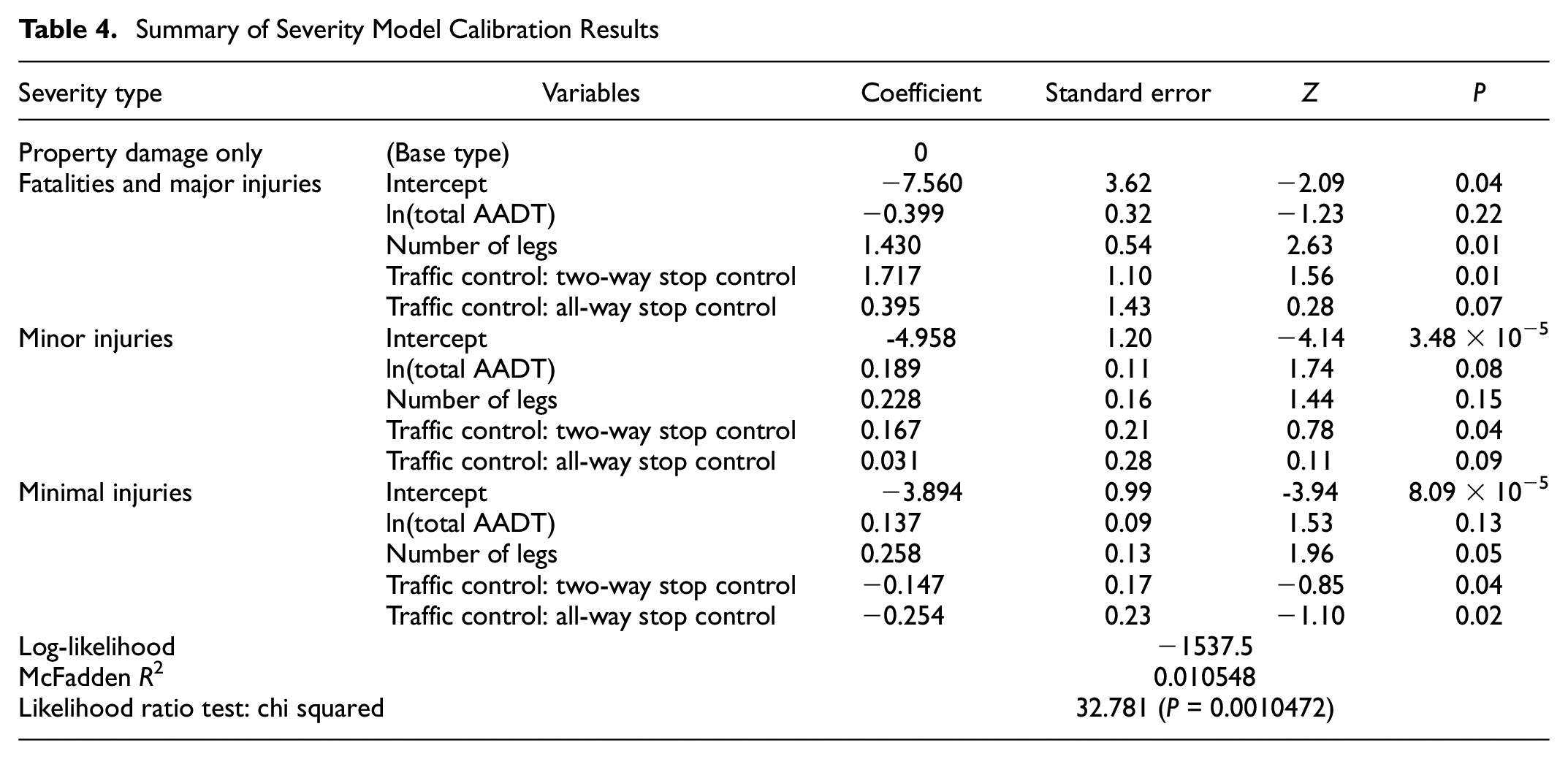
A multinomial logit model was calibrated based on crashes during the 5 years at all unsignalized intersections with any number of legs. Then, this calibrated model was used to estimate the probability associated with each collision severity at three-legged minor approach stop-controlled intersections.
Table 4 illustrates the model coefficients associated with each variable considered in the model. The model had three statistically significant variables: total traffic volume, number of legs, and traffic control type. Both all-way and two-way stop-controlled (minor approach stop-controlled in three-legged intersections) types were positively correlated with the probability of fatalities and major and minor injury levels.
Summary of Severity Model Calibration Results
CR for Ranking of Intersections Based on Total Risk
Each severity type was converted to a dollar value by assuming a nominal cost. De Leur ( 30 ) calculated the equivalent monetary of the average social cost of crashes by severity in 2018 as follows:
fatal crash: $2,389,953
major injury crash: $376,771
minor injury crash: $50,546
minimal injury crash: $32,041
PDO: $14,391.
Note that since the minimal injury cost has not been calculated in this study, we used the social cost defined in Vodden et al. ( 31 ) for this severity level. In this regard, we first calculated the growth rate of PDO cost between these two studies (i.e., 1.79); then, by multiplying the cost of minimal injury level in Vodden et al. ( 31 ), i.e., $17,900, by the calculated growth rate, we estimated the cost of minimal injury crashes.
By multiplying the lower and upper limits of the expected annual number of crashes (i.e.,
Joint Confidence Region (CR) for Ranking Based on 95% Confidence Interval (CI)
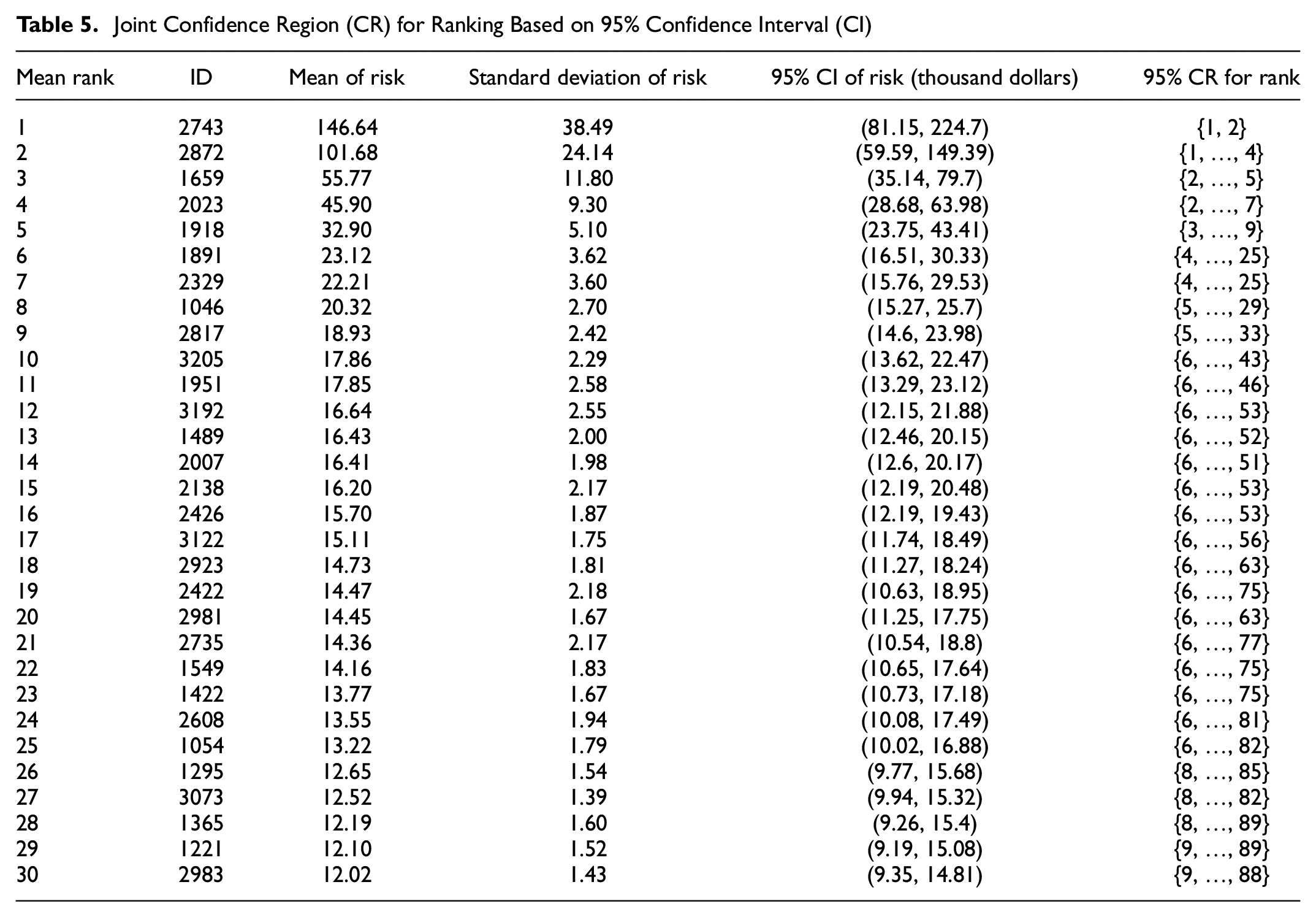
As an example, the results shown in Table 5 imply that, with a probability of 95%, the estimated annual risk for intersection #2872, will be in the range of $59,590 to $149,390. Moreover, it can be concluded that considering the mean of the estimated risk, this intersection will be selected as the second riskiest location, since its expected annual total risk is $101,680, which is $45,910 more than the second-ranked intersection (i.e., #1659). However, if the uncertainty in the expected total risk is taken into consideration, it could be ranked as the first, second, third, or even fourth riskiest location.
In addition, if the goal is to identify a list of hotspots based on a certain risk threshold value, the CIs of the estimated risk at the individual locations would provide more complete information for decision-making. In this case, the CI provides some underlying information about the safety of the location, which would not be captured if only the mean of the total risk were taken into account. As an example, suppose that the decision-makers wish to identify the hotspot locations with risk values exceeding $20,000 annually. If only the mean estimated risk value were used, as in the conventional approach, eight intersections would be identified as hotspots. As shown in Figure 3, however, when the 95% CI is taken into account, 15 intersections are categorized as hotspots.
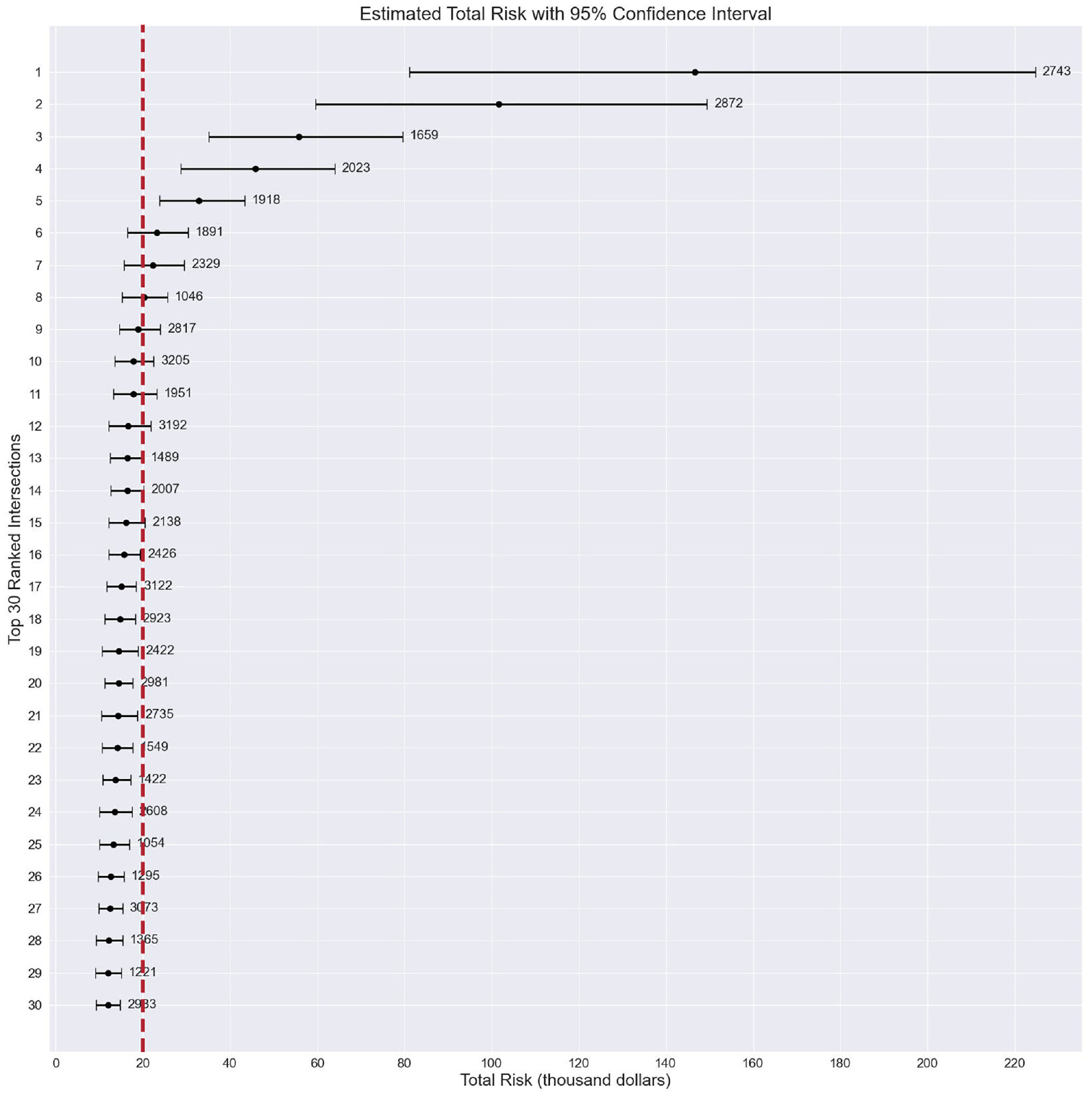
Estimated total risk with 95% confidence interval.
Conclusion
This study employed a frequentist approach to finding a joint CR for ranking locations of interest by risk and identifying crash hotspots. A case study on ranking three-legged stop-controlled intersections in Kitchener, Ontario, Canada, was conducted to show the benefits of the proposed approach. The crash frequency and severity of a given crash were estimated using a hierarchical FB NB model and a multinomial logit model, respectively. For each location, the CI of risk is obtained on the basis of the estimated 95% CI of the crash frequency and the predicted probability of each severity level. Based on the CR, individual intersections can be ranked accordingly with the additional consideration of uncertainty. Specifically, when uncertainty is considered, an intersection can have varied ranking positions with different probabilities, since the true value of its estimated crash risk follows a distribution. As a result, consideration of uncertainty in the road safety analysis may help identify more accurate hotspots for applying safety action items.
To our knowledge, there have been few studies on the integration of uncertainty in a network screening process; therefore, this study provides some insightful information for future researchers and practitioners who wish to incorporate uncertainty in their analyses. In this regard, the following research direction can be suggested for future studies:
This study developed a Bayesian model based on AADT for intersection crash predictions. However, additional predictors could be included to enhance accuracy. In addition, future studies may consider developing a Bayesian model to account for uncertainty in crash severity assessment and incorporating uncertainty introduced by the predictors.
This study used a simple method to fill in missing AADT data of road segments. While the estimated AADT had an acceptable level of accuracy, future studies could consider a better method, such as estimating traffic volumes based on available data in other crossed road segments, for more accurate prediction models.
In addition to the uncertainty associated with the modeling part, there are various sources of uncertainty resulting from the data. A wide range of variations in the estimated traffic volume (i.e., AADT) is one of these sources, and can affect the result of risk estimations. However, for simplicity, the effect of traffic volume uncertainty has not been investigated in this study and can be considered in future research.
In this study, we employed a frequentist model to determine a joint CR for the rankings of the locations. However, this CR can also be determined using the Bayesian framework.
In addition, conditional probability theory can also be employed to calculate the probability of getting each rank within the defined CR.
The application of the proposed methodology was demonstrated by applying it to three-legged minor approach stop-controlled intersections to identify hotspots with consideration of uncertainty. However, this method can be applied to all other types of roadway entity, which can be considered in future studies to compare the results of the analysis.
Footnotes
Acknowledgements
The authors acknowledge the City of Kitchener for their support in providing the crash and inventory datasets.
Author Contributions
The authors confirm contribution to the paper as follows: study conception and design: Aminghafouri, Fu; data collection: Aminghafouri; analysis and interpretation of results: Aminghafouri, Fu; draft manuscript preparation: Aminghafouri, Fu. All authors reviewed the results and approved the final version of the manuscript.
Declaration of Conflicting Interests
The author(s) declared no potential conflicts of interest with respect to the research, authorship, and/or publication of this article.
Funding
The author(s) received no financial support for the research, authorship, and/or publication of this article.