Sage Journals: Discover world-class research

Abstract

Asphalt concrete (AC) balanced mix design (BMD) is based on the selection of aggregate gradation, component volumetrics, and binder content to control pavement cracking and rutting potential. The Illinois Flexibility Index Test (I-FIT) and the Hamburg Wheel Tracking Test (HWTT) results, used to predict cracking and rutting potential, respectively, are used in the BMD approach. However, BMD generally relies on a trial-and-error process to identify the aggregate gradation and binder content needed to meet volumetrics and optimize I-FIT and HWTT results. Minimizing or eliminating the trial-and-error process would increase productivity and accuracy. Therefore, this study proposes an autoencoder deep neural network (ADNN) to develop optimized AC mix design alternatives that can meet a prescribed flexibility index (FI) and rut depth (RD). Autoencoders are a type of neural network designed for representation learning composed of an encoder and a decoder. The encoder detects a structured pattern in the original input data to create a compressed representation of the AC mix design. The decoder reconstructs the compressed representation. The proposed autoencoder is composed of an encoder of five hidden layers, a latent space of one node, and a five-hidden-layer decoder. Models were created from a database of 5,357 data sets that include mix properties, I-FIT FI, and HWTT RD (after data preprocessing was conducted). An autoencoder was then trained to predict the total binder content, and aggregate gradation based on a target mix type, FI, and RD.

Keywords

materials asphalt materials mix design performance tests pavements asphalt autoencoder

Superpave is a mix design method for asphalt concrete (AC) that has been widely used since the late 1990s. Since its development, the asphalt community has generally acknowledged the need for performance tests to address fatigue cracking, thermal cracking, and rutting. In the late 2000s, performance predictive tests were proposed to address the lack of cracking and rutting potential evaluation in Superpave. The Superpave Shear Tester (SST) and Indirect Tensile Tester (IDT) were proposed for AC mix design ( 1 ). Both tests were intended to be used alongside structural and traffic models to predict AC performance ( 2 ). However, limitations in the models and equipment costs prevented the implementation of SST and IDT. Therefore, only volumetric and moisture requirements for mix acceptance were recommended, which may not be sufficient to predict pavement performance ( 3 , 4 ). Because of using a trial-and-error process, the current AC mix design approach can be lengthy and inefficient.

The Illinois Flexibility Index Test (I-FIT) and the Hamburg Wheel Tracking Test (HWTT) were proposed to complement Superpave volumetric properties for AC mix acceptance ( 5 ). Since the 2020s, many states require the AC mixes to meet cracking and rutting performance test requirements. The AC design is discarded if it does not meet performance tests and volumetric requirements. Given that Superpave’s main limitation is its reliance on trial-and-error process for the selection of the AC properties needed to meet the volumetric and laboratory performance test requirements, neural networks could improve the selection of the AC design process.

Researchers have studied neural networks for AC mix design since the 2010s. Ozturk and Kutay ( 6 ) developed an artificial neural network (ANN) to predict Superpave AC volumetric properties based on gyration, aggregate gradation, bulk specific gravity of aggregates, binder grade, and binder content. A feed-forward (backpropagation) ANN model of three hidden layers was used. The model used 1,817 AC mixes from pavements constructed from 2008 to 2010 by the Nebraska Department of Transportation (DOT). The R² of the true versus predicted volumetric data ranged between 0.53 and 0.63. Sebaaly et al. ( 7 ) used an ANN with genetic optimization algorithms to develop a model that selects AC properties based on Marshall AC mix design requirements. The model used the ANN to predict air void content, theoretical maximum specific gravity, Marshall stability, and Marshall flow. The input parameters were aggregate gradation, binder content, binder grade, and aggregate bulk specific gravity. A genetic algorithm was then used to implement an optimization subroutine to recommend optimum binder content and aggregate gradation for a specific AC design. The models provided correlations with an R² of 0.93 to 0.96. Furthermore, Nguyen et al. and Othman ( 8 , 9) developed improved ANN models for the estimation of the Marshall Stability and Flow. To date, the AC mix design ANN models in the literature do not consider cracking and rutting potential predictive tests to optimize the selection of AC properties.

I-FIT and HWTT

I-FIT evaluates AC cracking susceptibility ( 10 ). The test is conducted by subjecting a semicircular AC sample to three-point bending at 25°C. AC specimens are sawn from Superpave gyratory compactor pills to create 50-mm-thick semicircular specimens with a diameter of 150 mm. The specimen has a 15-mm notch fabricated at the center ( 11 ). During the test, the AC specimen is placed over two rollers and a monotonic load is applied along the vertical diameter of the specimen at a displacement rate of 50 mm/min controlled by a linear variable differential transformer (LVDT) at a temperature of 25°C ( 10 ). The load versus displacement curve is measured using the LVDT and load cell measurements. The work of fracture ( $W_{f})$ , fracture energy ( $G_{f})$ , post-peak slope (m), and flexibility index (FI) can then be computed from the load versus displacement curve ( 10 , 12 , 13 ).

The HWTT simulates the permanent deformation (rutting) caused by cyclic loading ( 14 ). The test set-up consists of a steel wheel tracked over an AC sample submerged in water at a speed of 0.305 m/s (1 ft/s). The steel wheel is 203.2 mm (8.0 in.) in diameter, 47.0 mm (1.85 in.) wide, and applies a load of 705.0 ± 4.5 N (158.0 ± 1.0 lb). The test simulates the permanent deformation (rutting) of traffic. Tests are typically conducted on two AC specimens fabricated using a gyratory compactor ( 15 ). The wheel is tracked for up to 20,000 cycles or until the threshold of number of passes or rutting level is reached. During the test, rut depth is measured with an LVDT.

Autoencoders

There is a need to develop a model for automated AC mix design that predicts the mix properties based on cracking and rutting potential as measured by I-FIT and HWTT. Recent developments in ANN architectures, such as autoencoders, may be used. An autoencoder is an unsupervised deep neural network (DNN) composed of an encoder and a decoder (Figure 1). The encoder reduces the dimension of the original input to a latent space ( 16 ). The decoder reconstructs the input based on the encoded representation. The encoder is forced to extract the primary components of the input and eliminate the corruptions (noise) that the training data contains. The decoder then reconstructs a denoised version of the input to the model ( 16 ).

Figure 1.

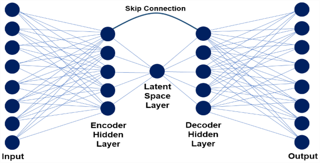
Theoretical autoencoder composed of one encoder hidden layer, one decoder layer, and a latent space of one node.

Autoencoders were initially developed for image “denoising” and analysis. The autoencoder structure is designed to learn the image features and encode the images in the latent space ( 16 ) Initial applications consist of training autoencoders with un-noised images, after which noisy or corrupted images are passed through. The autoencoder detects the noisy image features and returns a reconstructed “clean” version of the noisy image ( 16 ). The number of nodes of the input and output layer of the autoencoder is the same as the number of pixels in an image. In the input, the “Red-Green-Blue” or “Greyscale” values of the images are inputs. In the output, the reconstrued image is delivered with the new “Red-Green-Blue” or “Greyscale” values per pixel.

Autoencoders can detect and encode a specific pattern that a matrix of numbers can contain. Since the 2020s, autoencoders have been used for various civil engineering applications. Ba-Alawi et al. ( 17 ) used variational autoencoders to backfill missing data and detect faults in wastewater treatment plant (WWTP) sensors. The data contained 18 readings from WWTP with either noise or faulty sensor readings. The model encoded the data to one node which stored complex features from WWTP data. Boquet et al. ( 18 ) used variational autoencoders to encode traffic data to a two-dimensional latent space that can then be used for data traffic forecasting and to replace missing data. The latent space learns a probability distribution of the traffic data. Then, encoded data can be used to forecast traffic. Similarly, Yuan et al. ( 19 ) developed autoencoders to impute the missing traffic data in the generator of an adversarial network aimed at forecasting traffic. Like images, wastewater, and traffic, AC mix designs are also composed of a unique combination of input variables with a unique data structure that an autoencoder can detect.

Objective and Scope

The objective of this study was to develop an ADNN for AC mix design. The ADNN model was developed to learn the pattern of a distribution of a known set of representative AC mixes (training) and encode it. The encoded space is then used to decode AC mix designs for a prescribed cracking and rutting potential as measured by I-FIT and HWTT. During training, the encoder layers of the model create a latent space to store the training mix information while the decoder reconstructs an AC mix design to predict binder content, volumetrics, and aggregate gradation. After training, the autoencoder receives the target mix type, gyrations, binder grade, recycled materials content, FI, and rut depth to predict an AC mix design capable of fitting these performance predictive parameters.

To date, autoencoders have not been used for AC design data. Using this model would allow the ability to use mix design data for encoded and decoded, similar to other data structures as images, to be determined.

Database and Data Preprocessing

The original data, compiled by the Illinois Department of Transportation (IDOT), contained a total of 18,562 I-FIT data sets from 2,201 AC mix designs collected between 2016 and 2020. A total of 8,117 HWTT data sets were collected from 3,772 AC mix designs dating from 2010 to 2020. The database preparation was detailed in Rivera-Pérez and Al-Qadi ( 20 ). The database contained 26 mix parameters, summarized in Table 1. The I-FIT data sets include fracture energy, slope, and FI data. The HWTT data sets include the minimum number of passes required to reach the threshold in accordance with IDOT specifications ( 21 ). Table 1 summarizes the impact of FI and rut depth as reported in Rivera-Pérez and Al-Qadi ( 20 ). The AC aggregate gradation data were collected per ( 22 ).

Table 1.

Summary of the I-FIT and HWTT DNN Inputs

Feature	Input		Range	Type	Label	I-FIT	HWTT
1	AC versus SMA		AC, SMA	Categorical	acsma	SMA improves FI	SMA reduces rutting.
2	NMAS		4.75, 9.5, 12.5. 19.0 mm	Numerical	nmas	Increased NMAS deteriorates FI	Increased NMAS reduces rutting.
3	Pavement layer		Surface Course (SC), Binder Course (BC), Leveling Binder (LB)	Categorical	lta	SC improves FI more than BC	BC reduces rutting more than SC
4	Number of gyrations		30, 50, 70, 80, 90	Numerical	mix_number	Increases gyration deteriorates FI.	Increases gyration reduces rutting.
5	Binder grade	High	76, 70, 64, 58, 52, 46	Numerical	binder_high		Greater high grade reduce rutting
6	Binder grade	Low	−34, −28, −22	Numerical	binder_low	Smaller (more negative) low grade improves FI
7	AC content		4 to 9	Numerical	Ac_content	Increased binder content improves FI	Increased AC contentincreases rutting
8	Binder polymer modified		Yes or no	Categorical	modified	Polymer Modified binder improves FI	Polymer Modified binder reduces rutting
9	Asphalt binder replacement (ABR)		0 to 50	Numerical	abr	Increased ABR deteriorates FI	Increased ABRreduces rutting.
10	Recycled asphalt pavement (RAP)		0 to 40	Numerical	rap_frap	Increased RAP deteriorates FI	Increased RAPreduces rutting
11	Recycled asphalt shingles (RAS)		0 to 23	Numerical	ras	Increased RAS deteriorates FI	Increased RASreduces rutting
12	Bulk specific gravity (G_mb)		2.175 to 2.952	Numerical	gmb	Inconclusive	Inconclusive
13	Theoretical maximum specific gravity (G_mm)		2.354 to 3.120	Numerical	gmm	Increased G_mm deteriorates FI	Increased G_mm reduces rutting
15	Air voids (AV)		4 to 8.7	Numerical	av	Increased AVimproves FI	Increased AVincreases rutting.
16	Field voids in mineral aggregate (VMA)		14.5 to 23,0	Numerical	vma_field	Increased VMA improves FI	Increased VMAincreases rutting.
17	Volume of binder effective (V_be)		7.5 to 17	Numerical	vbe	Increased V_be improves FI	Increased in V_be increases rutting
18	Aggregate gradation sieves (mm)	12.5	95 to 100	Numerical	12.5	Increased percent retained in sieve 9.5- and 0.075-mm deteriorates FI.Impact of other sieves was unconclusive.	Increased percent retained in sieve 0.3- and 0.15-mm (fine component) reduces rutting..
19		9.5	75 to 100	Numerical	9.5
20		4.75	40 to 75	Numerical	4.75
21		2.36	15 to 53	Numerical	2.36
22		1.18	10 to 40	Numerical	1.18
23		0.6	6 to 60	Numerical	0.6
24		0.3	7 to 16	Numerical	0.3
25		0.15	4.5 to 12.5	Numerical	0.15
26		0.08	3 to10.5	Numerical	0.075

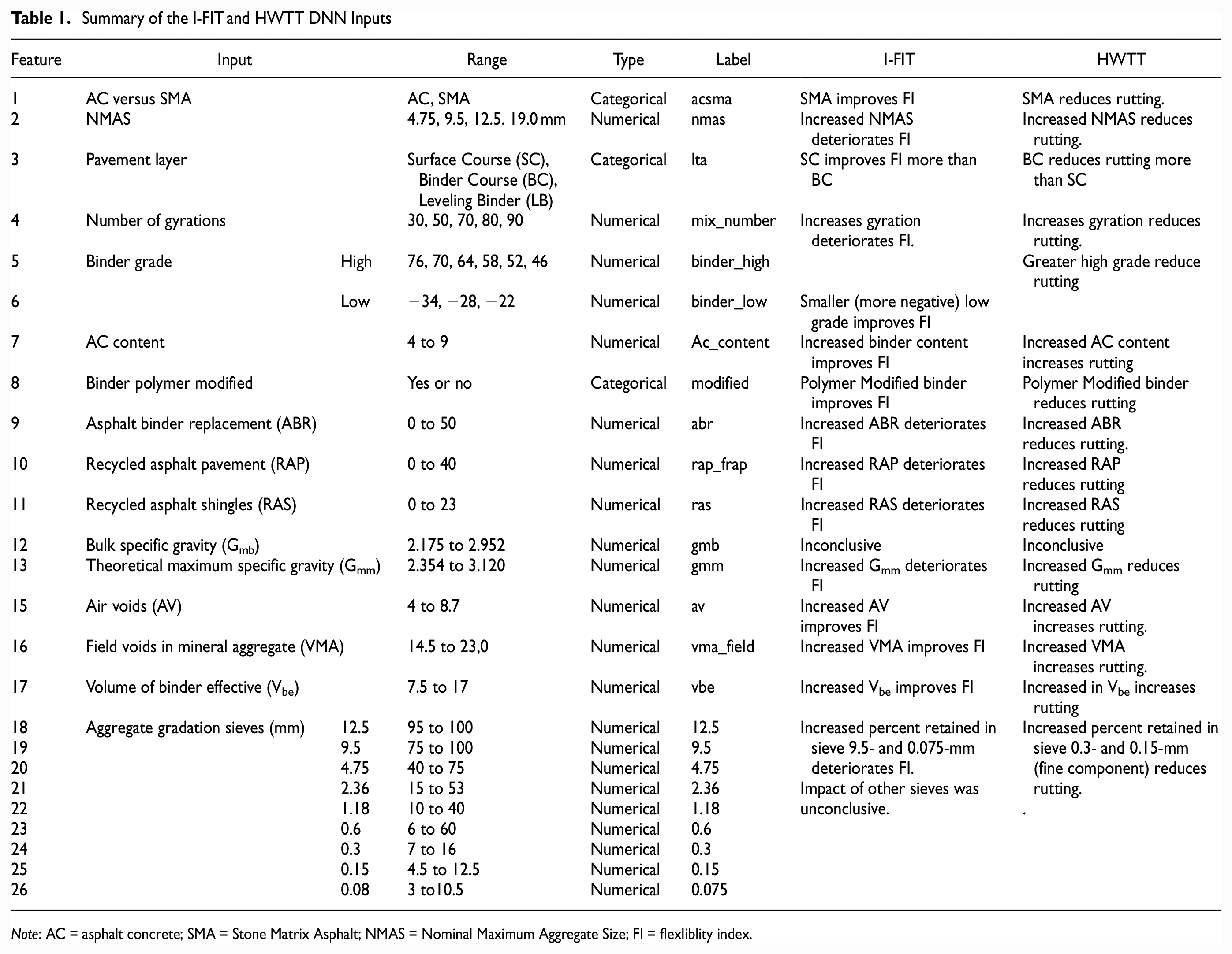
Note: AC = asphalt concrete; SMA = Stone Matrix Asphalt; NMAS = Nominal Maximum Aggregate Size; FI = flexliblity index.

Data preprocessing was conducted through cleaning and transformation procedure detailed in Rivera-Pérez and Al-Qadi ( 23 ). The procedure consisted of the following steps.

Step 1: Removal of test replicate outliers of each AC mix design in accordance with the interquartile range method described in Vinutha et al. ( 24 ).

Step 2: Removal of all the test replicates of AC mixes with a coefficient of variation that exceeded 50% for FI or 40% for rut depth.

Step 3: Removal of data sets that were long-term aged (LTA) ( 25 ).

Step 4: Transformation from aggregate percent passing to aggregate percent retained for all aggregate gradations in accordance with Equation 1 below:

% R e t a i n e d S i e v e_{i} = % P a s s i n g S i e v e_{i} - % P a s s i n g S i e v e_{i + 1}

(1)

Step 5: “One hot” encoding was applied to the “AC versus SMA,”“Pavement Layer,” and “modified” labels of the database.

Step 7: Conduct the “Yeo-Johnson” transformation ( 26 ) and apply scaling. The “Yeo-Johnson” method transforms a continuous (numeric) variable to a Gaussian (normal) distribution. A “MinMax” scaler was used afterward to scale the data in decimals that ranged from 0 to 1 ( 27 ). The transformation allows for the reduction of skew in the raw variables.

Step 8: Select data sets of AC mixes that contained FI and rut depth reported for the final ADNN training and testing database.

The specific details and motivation for conducting this procedure are provided in detail in Rivera-Pérez and Al-Qadi ( 23 ). After data preprocessing (including data cleaning and transformation), a final database of 5,357 I-FIT and HWTT data sets was used to develop the ADNN.

ADNN Model Development

Model Metrics

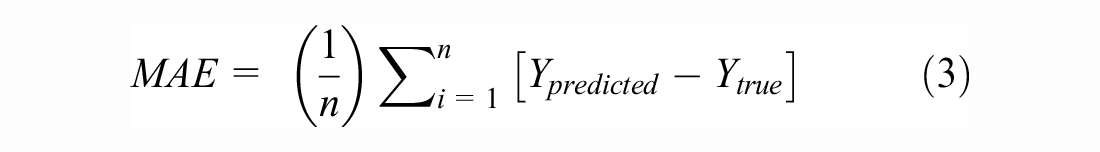
The mean squared error (MSE) was selected as the loss function for model training. The ADNN is a multiple-input multiple-output (MIMO) structure with 27 output parameters. As such, the loss function iterates over the number of observations and number of outputs as shown in Equation 2:

MSE = (\frac{1}{m}) \sum_{i = 1}^{m} (\frac{1}{n}) \sum_{i = 1}^{n} (Y_{predicted} - Y_{true}) \hat{2}

(2)

where

m is number of model outputs ( 27 ),

n is the number of training data sets,

$Y_{predicted}$ is either the reconstructed or predicted value, and

$Y_{true}$ is the true value.

The outputs were scaled to avoid disproportionate attribute contributions during the MSE loss function calculation.

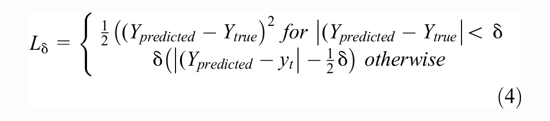
The mean absolute error (MAE), average of sum of residuals, and Huber loss were used as evaluation metrics for the model testing. During model testing, the MSE, MAE, and Huber loss were calculated independently for each of the 27 outputs to evaluate where the model struggled in either predicting or reconstructing AC mix design values. The residuals refer to the differences between the reconstructed and predicted values ( $Y_{predicted}$ ) and the true value ( $Y_{true})$ for “n” number of observations (Equation 3).

MAE = (\frac{1}{n}) \sum_{i = 1}^{n} [Y_{predicted} - Y_{true}]

(3)

The Huber loss ( $L_{δ})$ was used to reduce the influence of outliers into the measurement of the model error (Equation 4). The hyper-parameter, δ (delta), which can be tuned, determines how small that error must be to make it quadratic ( 28 ). Huber loss approaches MAE when δ is approximately zero and MSE when δ is approximately infinity (large numbers). Therefore, the effect of prediction outliers has a lesser impact than the error measurement.

L_{δ} = {\begin{matrix} \begin{matrix} \frac{1}{2} {((Y_{predicted} - Y_{true})}^{2} for | (Y_{predicted} - Y_{true} | < δ \\ δ (| (Y_{predicted} - y_{t} | - \frac{1}{2} δ) otherwise \end{matrix} \end{matrix}

(4)

Input and Output Selection

The inputs layer of the ADNN consists of a one-dimensional (1-D) layer of 27 nodes, one for each AC mix design parameter. The output layer has the same dimension as the input layer to allow the model to reconstruct new AC mix designs. The autoencoder structure allows for different input and output structures. The number of nodes in the last layer could have a different dimension than the input. In this study, the autoencoder had the same number of inputs and outputs to follow a construction and reconstruction of the mix. During input/output layer design, the mix parameters were separated into two groups: “Known” and “Unknown” parameters. Figure 2 presents an example data set for the input and output layer to illustrate the differences between these two groups. The “Known” parameters are AC mix design properties that the AC designers know before designing a mix. “Known” properties are typically specified in the contract and are inputs of the model. The model receives these parameters to be encoded in the latent space during training. The ADNN then has the capacity to “reconstruct” the “known” properties in the output layer to the same value that was input, or a close approximation as shown in Figure 2. “Unknown” parameters are the properties that the model is intended to predict. The “unknown” parameters are input to the model as missing values of AC mix design (input as “0”) that the model is intended to “predict” as shown in Figure 2.

Figure 2.

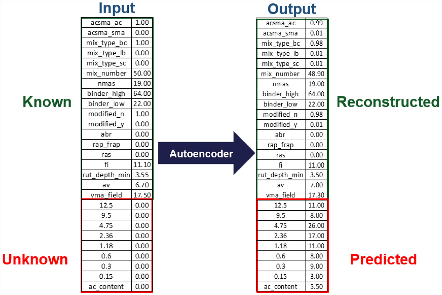
Example of an input data set and the model expected output.

The “known” properties of the ADNN are the following: AC versus SMA, NMAS, binder polymer modified, pavement layer, number of gyrations, binder high, binder low, Asphalt binder replacement (ABR), air voids (AV), voids in mineral aggregate (VMA), recycled asphalt pavement (RAP), recycled asphalt shingles (RAS), I-FIT FI, and Hamburg RD. The “unknown” properties to be “predicted” by the model are the following: total binder content, and the aggregate percent retained in sieves 12.5, 9.5, 4.75, 2.36, 1.18, 0.6, 0.3, and 0.15. One hot encoding determined that AC versus SMA, polymer modification, and pavement layer use two, two, and three nodes per parameter, respectively.

There were two alternatives for inputting the training data during model training. The first alternative is using the training data set without removing the “unknown” variables from the autoencoder for model training. The second alternative is removing the “unknown” parameters from the training data and replacing them with a neutral value chosen as “0” for this study. The second alternative resembles the model work with the testing data. During model testing the “unknown” values are always removed from the testing data to allow the model to predict the AC mix design.

The second alternative was chosen, in which the model is trained using the missing values. Preliminary model testing was done using 11 hidden layer ADNN structure. It was found that the second alternative caused an average decrease of 85% in the model test MSE after converging. One possible reason is that the model trained with complete data will not be able to detect that the “0” values used in the volumetrics and aggregate gradation are dummy and that the model should replace them with the complete information.

In summary, the model received 27 inputs and 27 outputs which include “known” and “unknown” parameters. During model training, the input vector of each AC mix design had the “unknown” parameters removed and replaced with “0.” The model was then tasked with predicting the “unknown” parameters and reconstructing the parameters that were given to it.

Hidden Layer Selection

Encoder-Decoder

The number of hidden layers was empirically determined. Preliminary testing was conducted on five model alternatives to determine an optimum number of hidden layers for the model. The five alternatives consisted of symmetric layer structures between the encoder and decoder. In the encoder, the number of nodes is reduced by a fixed interval until it reaches a central node of 1 (latent space). Then, in the decoder, the number of nodes increases by the same interval until reaching the size of the output layer. The node reduction intervals of 15, 10, 5, 2, or 1 were considered.

During the hidden layer selection, the adaptive moment estimation (ADAM), with a learning rate of 0.001 and a batch size of 32, was used ( 29 ). The learning rates of 0.01 and 0.0001 were attempted but did not achieve better performance than 0.001. A rectified linear activation function (ReLU), as defined by Chai and Draxler ( 30 ), was used for the hidden layers. For the output layer, the sigmoid function was used as the data were scaled between 0 to 1. The training data were split between 80% for training and 20% for testing.

The preliminary models that were tested excluded skip connections to optimize hidden layers’ accuracy alone. Table 2 summarizes the MSE of the model. As the number of hidden layers increased, the MSE decreased in the first three alternatives. However, for alternatives four and five the model was unable to train. As reported in the literature, autoencoders with many hidden layers are susceptible to gradient vanishing, which causes the model to be unable to successfully train ( 16 ). The final structure of the model consisted of 11 hidden layers. The number of nodes for the 11 layers were: 25, 20,15, 10, 5, 1, 5, 10, 15, 20, and 25.

Table 2.

Average Test MSE for Five Model Alternatives with Different Numbers of Hidden Layers

Alternative	Hidden layers	Node reduction interval	Average test MSE for “predicted” parameters
1	3	15	0.012
2	5	10	0.011
3	11	5	0.009
4	29	2	-
5	57	1	-

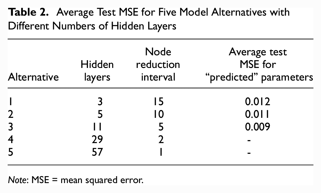
Note: MSE = mean squared error.

Latent Space

The number of nodes needed to encode AC mix design in the central layer was evaluated. Three models with a central layer of one, two, or three nodes were tested. The hidden layer structure of 11 hidden layers was used for the three preliminary models. It was found that the MSE for these three alternatives was the same at 0.008. A single central node was chosen to encode the data in the smallest dimension possible.

Skip Connections

To reduce the susceptibility of gradient loss, skip connections were added between two corresponding (i.e., the same number of nodes) encoder and decoder layers. Skip connections allow for the recovery of AC mix design details that have been lost during encoding ( 31 , 32 ). In addition, skip connections allow for the backpropagation of the gradient during training, which helps to find a better minimum. This overcomes the problem of gradient vanishing seen in the hidden layer selection.

An evaluation was conducted to determine the encoder-decoder layer pairs that were going to be connected. The options available were connecting the encoder-decoder layers with either 25, 20, 15, 10, or 5 nodes for the 11-layer model structure previously selected. In addition, the input layer can have a direct skip connection with the output layer (I/O skip connection). Figure 3 presents the MSE for the 12 reconstructed parameters. The MSE for a similar model of 11 layers with no skip connections is also shown (“no skip”). The skip connections reduced the MSE of the parameters to be predicted. The skip connection between layers of 25 nodes, which are the layers closer to the input and output, caused the most reduction to the MSE of the predicted parameters.

Figure 3.

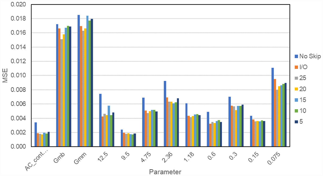
Mean squared error (MSE) of seven model alternatives that had a skip connection between the hidden layers of no skip connection, input/output layer, 5, 10, 15, 20, and 25 nodes.

A skip connection between the input and output layer causes the parameters “known” to the model to be transferred directly to the output layer. This causes an MSE of 0 for the parameters that are imputed to the model (AC versus SMA, NMAS, binder polymer modified, pavement layer, number of gyrations, binder high, binder low, ABR, AV, VMA, RAP, RAS, FI, and RD).

Based on Figure 3, two skip connections were recommended for final model, the first placed between the input and output layer to transfer the input parameter to the model output. This allows the model to focus its training on improving the accuracy of the parameters to be predicted. A second skip connection between the layers of 25 nodes improves the MSE of the parameters predicted by the model.

Model Summary and Training

Figure 4 presents the final ADNN architecture. The models were developed using the “Keras Functional Application Programming Interface” which allows the adding of skip connections in the Python TensorFlow library. The final model has 11 hidden layers, in which five are the encoder, five are the decoder, and one is the latent space. Two skip connections were added, the first between the input and output layers and the second between the encoder and decoder layers of 25 nodes.

Figure 4.

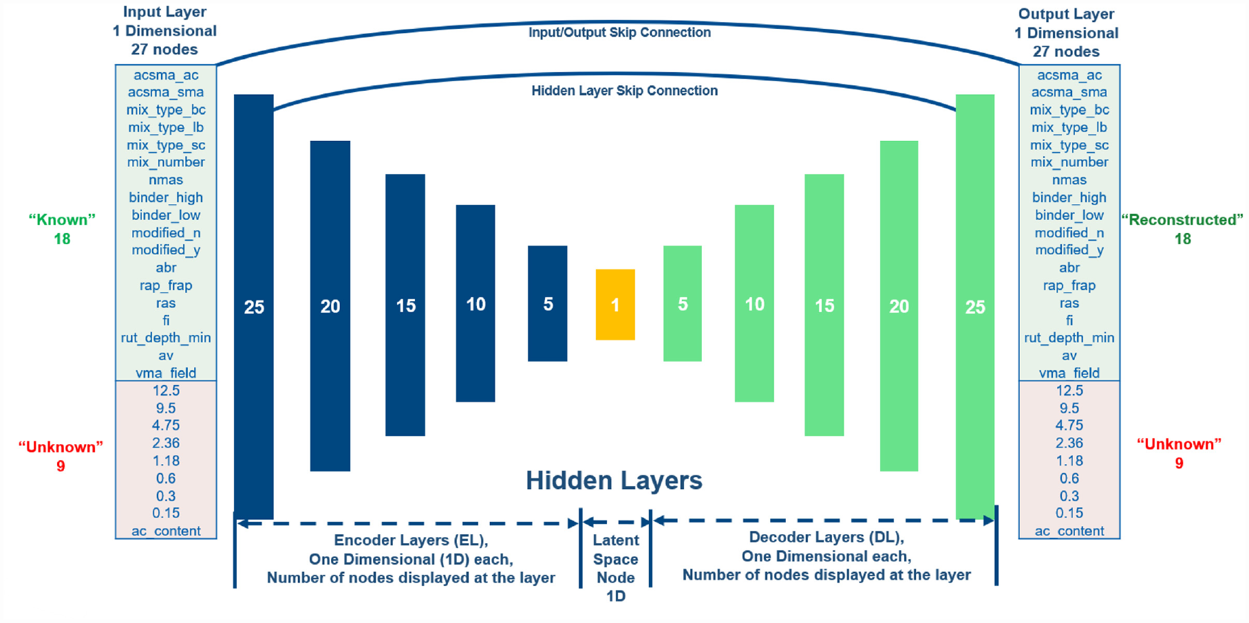
Diagram of the final autoencoder deep neural network (ADNN) architecture.

The ADNN was trained using 300 epochs. Twenty percent of the training data were used for validation. The ADAM optimization with a learning rate of 0.001 and a batch size of 32 was used ( 29 ). The MSE was monitored as a function of the training epochs as presented in Figure 5. The rectified linear activation function (ReLU) as defined by Agarap ( 33 ) was used for the hidden layers. For the output layer, the sigmoid function was used because the data were scaled between 0 to 1. Sigmoid provided smaller MSE than the linear function. The training data were split between 80% for training and 20% for testing.

Figure 5.

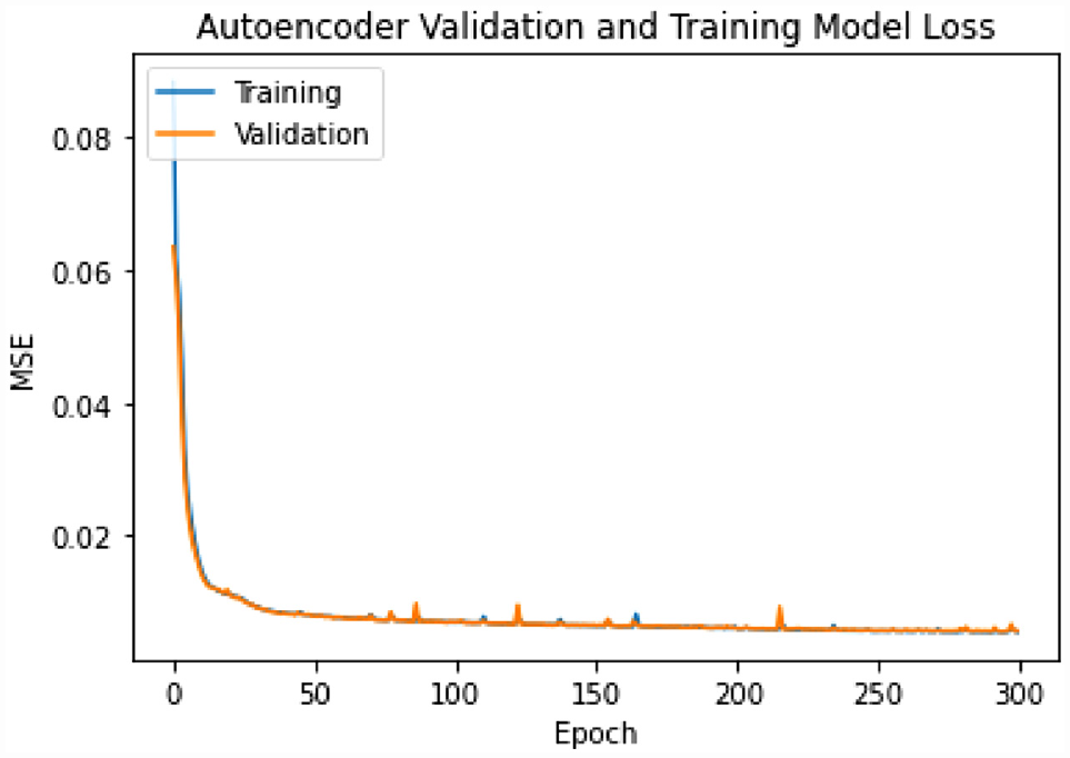
MSE versus epoch for the training of the ADNN model.

Model Results

Prediction Accuracy

Figures 6 and 7 present the true versus predicted plots for the six “reconstructed” and eight “predicted” parameters, respectively. Figure 6 shows that for the parameters that were “known” to the model, the autoencoder uses the exact value that was imputed in the AC mix design output. This is a direct result of the skip connection added between the input and output layers of the model. For the parameters that were predicted, these parameters were input as “0” on the model testing. The model can recognize that “0” is a dummy value and can automatically provide a prediction based on the “known” parameters input to the model. Therefore, the ADNN performs a task similar to rebuilding an image, but in this case building a reconstructed version of the AC mix design.

Figure 6.

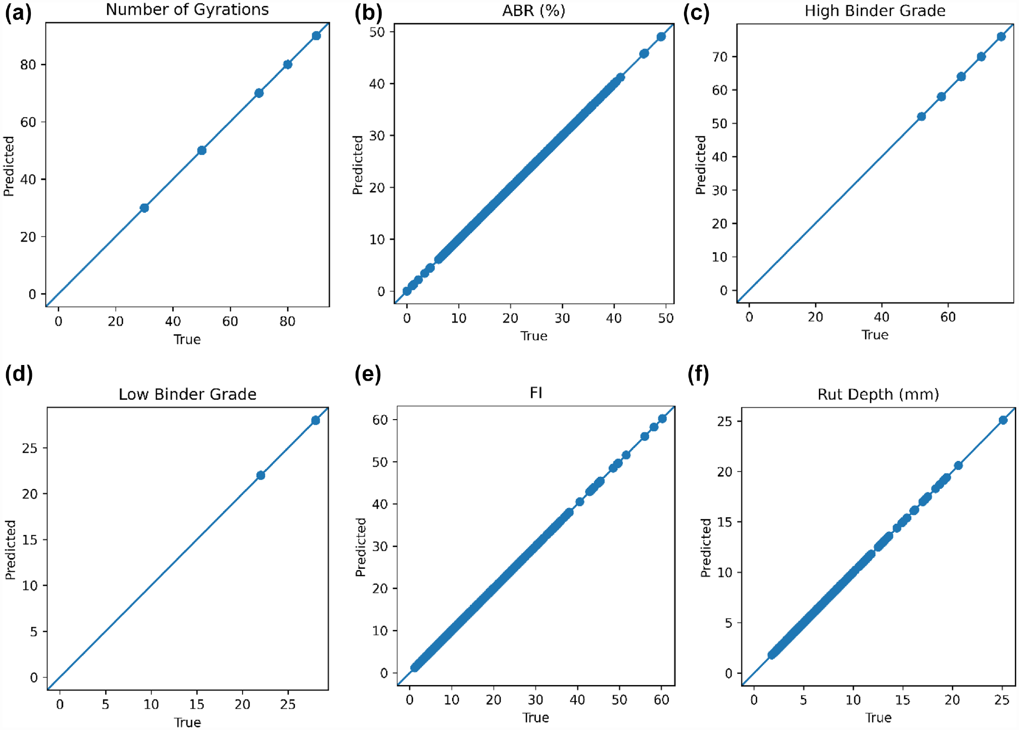
Predicted versus the true plot for six “known” parameters: (a) number of gyrations; (b) ABR; (c) high binder grade; (d) low binder grade; (e) FI; and (f) RD (1,071 data sets).

Figure 7.

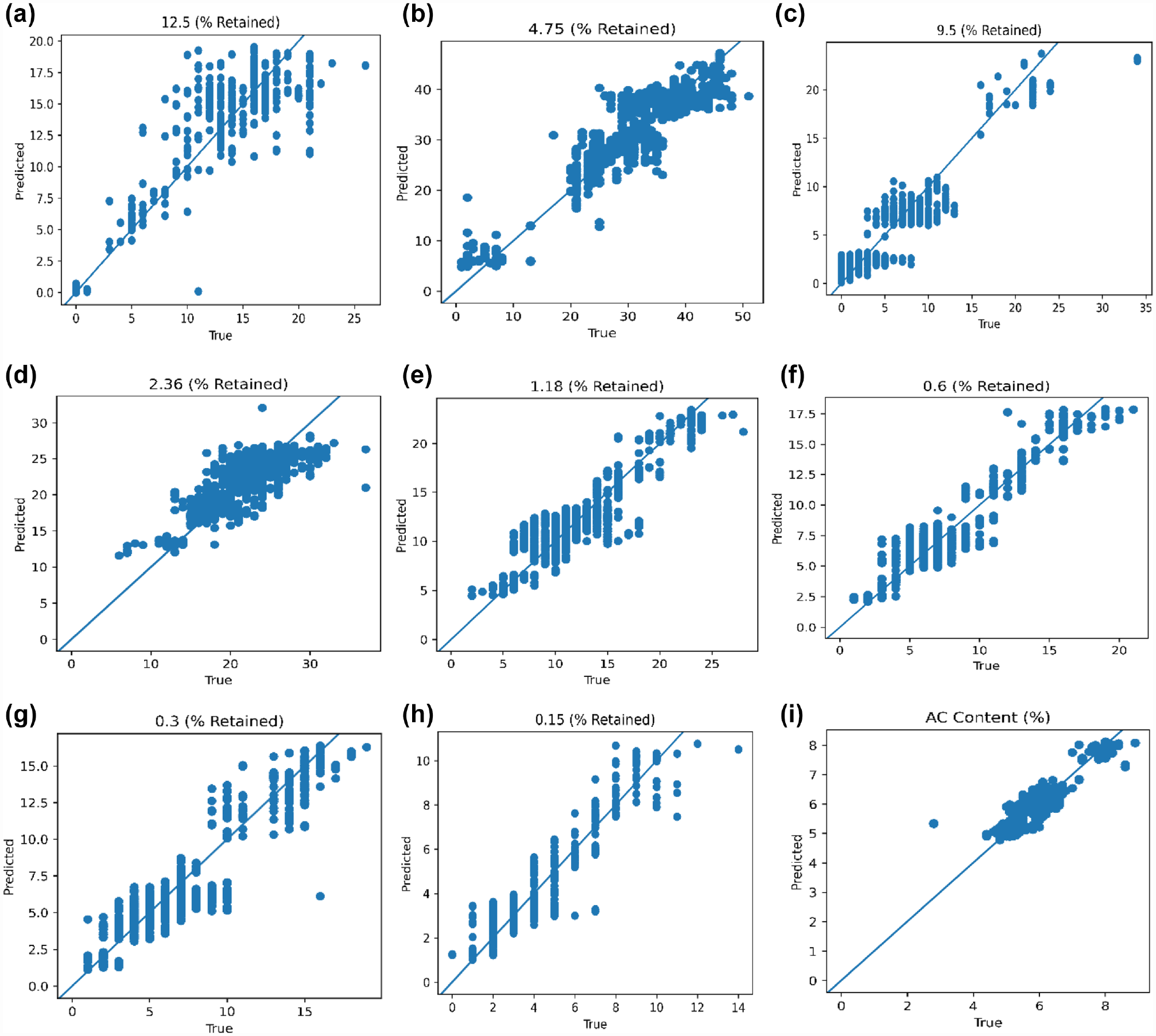
Predicted versus the true plot for eight “unknown” parameters: (a) 12.5 mm; (b) 9.5 mm; (c) 4.75 mm; (d) 2.36 mm; I 1.18 mm;(f) 0.6; (g) 0.3; (h) 0.15 mm; and (i) binder content (1,071 data sets).

Table 3 presents the evaluation metrics results for the parameters that were predicted in the test data used in the autoencoder. The evaluation metrics were computed on the scaled data to allow for the comparison of parameters that had different ranges. The AC content and aggregate gradation predictions were in acceptable ranges. For the aggregate percent passing 0.075 mm, Rivera-Pérez and Al-Qadi ( 20 ) found that the aggregate percent passing in this sieve was less likely to affect the FI and RD compared with other percentages. Therefore, a model based on FI and RD to predict the aggregate percent passing would struggle to predict the aggregate percent passing at the 0.075 mm sieve and was not considered in this study.

Table 3.

Evaluation Metrics Results for the Parameters to be Predicted in the Test Data of the ADNN (1,071 data sets)

	Not Scaled			Scaled
Parameter	MAE	MSE	Huber Loss	MAE	MSE	Huber loss	R²
AC (%)	0.184	0.065	2.596	0.008	0.003	0.001	0.80
12.5	0.781	2.561	0.312	0.002	0.005	0.002	0.88
9.5	1.11	2.356	0.442	0.002	0.004	0.002	0.75
4.75	2.644	12.712	1.204	0.002	0.008	0.005	0.85
2.36	1.811	5.659	0.788	0.001	0.004	0.003	0.80
1.18	4.259	2.947	0.531	0.007	0.005	0.003	0.81
0.6	0.854	1.303	0.321	0.003	0.004	0.002	0.86
0.3	0.979	1.655	0.376	0.003	0.005	0.002	0.74
0.15	0.55	0.532	0.175	0.002	0.002	0.001	0.76

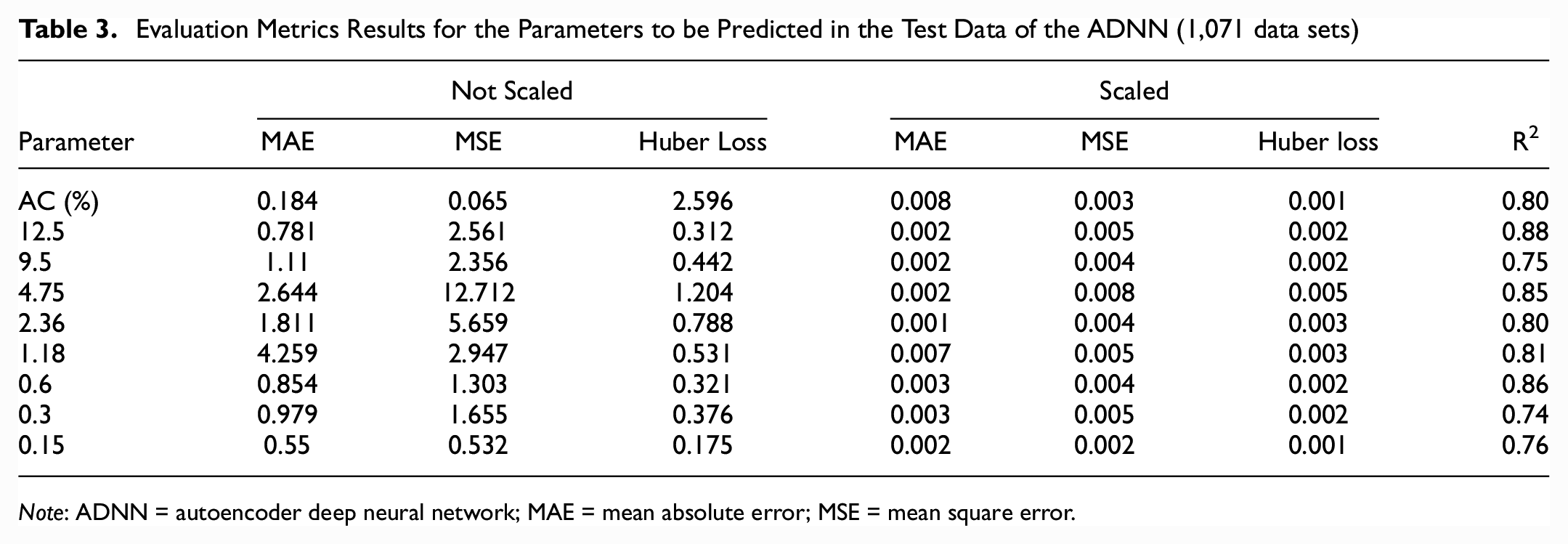
Note: ADNN = autoencoder deep neural network; MAE = mean absolute error; MSE = mean square error.

Model Limitations

The produced AC mix designs are bounded to the constraints of IDOT specifications (2022). IDOT requires 4% air voids at the design number of gyrations. However, the specimens are compacted at 7% air void content for I-FIT and HWTT. Therefore, the VMA and AV used to develop the model correspond to laboratory-compacted to represent “field” VMA and AV where the target is 7% for AV. The bounds of the database shown in Table 1 also apply to the model. Extrapolation is not recommended outside of these bounds.

Conclusion

This study used a relatively large database of AC cracking and rutting test data to develop an ADNN capable of creating new AC mix designs. I-FIT and HWTT data were collected by Rivera-Pérez and Al-Qadi ( 23 ) and compiled for the development of machine learning models for I-FIT and HWTT. A total of 5,357 post-processed data sets with complete RD and FI data were used to develop the model. The ADNN was developed with two objectives. First, the model receives an incomplete AC mix design. The “known” properties of the design were the AC versus SMA, NMAS, binder polymer modified, pavement layer, number of gyrations, binder high, binder low, ABR, AV, VMA, RAP, RAS, FI, and RD. The model predicts the “unknown” properties based on the inputs provided to the model. The “unknown” to be “predicted” by the model are binder content and aggregate percent retained in sieves 12.5, 9.5, 4.75, 2.36, 1.18, 0.6, 0.3, and 0.15.

The ADNN model structure chosen consisted of 11 hidden layers. Five hidden layers served as an encoder which reduced the dimension of the AC mix design to a latent space of one node in the central layer of the structure. Then a decoder reconstructed the AC mix design to an output of 27 nodes. Two skip connections were added to the model. The first connection linked the input and output layers. The second connection linked the first encoder hidden layer with 25 nodes to the last hidden layer of the decoder of 25 nodes. The input and output layer skip connection allowed for the use of the “known” properties input to the model directly in the output AC mix design. The results indicated that the model is able to provide acceptable predictions of aggregate gradation and binder content within the variability of FI and RD data.

Footnotes

Acknowledgements

The research was conducted in cooperation with the Illinois Department of Transportation (IDOT). The authors appreciate the help of IDOT Materials technicians and engineers in all District and Central Bureau of Materials laboratories for providing the data used to build the database. The contents of this paper reflect the view of the authors, who are responsible for the facts and the accuracy of the data presented here. The contents do not necessarily reflect the official views or policies of the Illinois Center for Transportation or the Illinois Department of Transportation.

Author Contributions

The authors confirm contribution to the paper as follows: study conception and design: J. Rivera-Pérez, A. Talebpour, and I. L. Al-Qadi; data collection: J. Rivera-Pérez; analysis and interpretation of results: J. Rivera-Pérez and A. Talebpour; draft manuscript preparation: J. Rivera-Pérez and I. L. Al-Qadi. All authors reviewed the results and approved the final version of the manuscript. The author(s) do not have any conflicts of interest to declare.

Declaration of Conflicting Interests

The author(s) declared no potential conflicts of interest with respect to the research, authorship, and/or publication of this article.

Funding

The author(s) disclosed receipt of the following financial support for the research, authorship, and/or publication of this article: Study data was provided by the Illinois Department of Transportation.

ORCID iDs

José Rivera-Pérez

Imad L. Al-Qadi

Data Availability Statement

The data that support the findings of this study are available on request from the Illinois Department of Transportation. The data are not publicly available as a result of proprietary restrictions by IDOT. A data request may be filled to IDOT’s Central Bureau of Materials and Physical Research.

References

May

R. W.

Anderson

R. M.

Perdomo

Comparison of SUPERPAVE with Conventional Pavement Design. Proc., Eighth International Conference on Asphalt Pavements Federal Highway Administration, University of Washington Press, 3rd edition (January 1, 1997), Seattle, Washington, 1997, p. 2.

Witczak

M. W.

Von Quintus

H. L.

Schwartz

C. W.

Superpave Support and Performance Models Management: Evaluation of the SHRP Performance Models System. Proc., Eighth International Conference on Asphalt Pavements Federal Highway Administration, University of Washington Press, 3rd edition (January 1, 1997), Seattle, Washington, 1997, p. 3.

Cominsky

R. J.

Killingsworth

B. M.

Anderson

R. M.

Anderson

D. A.

Crockford

Quality Control and Acceptance of Superpave-Designed Hot Mix Asphalt. National Cooperative Highway Research Program (NCHRP) Project, NCHRP Report 409. National Academies Press, Washington D.C., 1997.

Brown

E. R.

Kandhal

P. S.

Zhang

Performance Testing for Hot Mix Asphalt. NCAT Report 01-05. National Center for Asphalt Technology, Auburn, AL, 2001.

Barry

M. K.

Al-Qadi

I. L.

Ozer

Safi

An Implementation of the Illinois Flexibility Index Testing Protocol for Balanced Asphalt Mix Designs. In Bearing Capacity of Roads, Railways and Airfields ( Loizos

Al-Qadi

Scarpas

A. T.

Scarpas

A. T.

, eds.), CRC Press, London, 2017, pp. 217–221.

Ozturk

H. I.

Kutay

M. E.

An Artificial Neural Network Model for Virtual Superpave Asphalt Mixture Design. International Journal of Pavement Engineering, Vol. 15, No. 2, 2014, pp. 151–162.

Sebaaly

Varma

Maina

J. W.

Optimizing Asphalt Mix Design Process Using Artificial Neural Network and Genetic Algorithm. Construction and Building Materials, Vol. 168, 2018, pp. 660–670.

Nguyen

H. L.

T. H.

Pham

C. T.

T. T.

L. S.

V. M.

Pham

B. T.

H. B.

Development of Hybrid Artificial Intelligence Approaches and a Support Vector Machine Algorithm for Predicting the Marshall Parameters of Stone Matrix Asphalt. Applied Sciences, Vol. 9, No. 15, 2019, p. 3172.

Othman

Prediction of the Hot Asphalt Mix Properties Using Deep Neural Networks. Beni-Suef University Journal of Basic and Applied Sciences, Vol. 11, No. 1, 2022, pp. 1–14.

10.

Al-Qadi

I. L.

Ozer

Lambros

El Khatib

Singhvi

Khan

Rivera-Perez

Doll

Testing Protocols to Ensure Performance of High Asphalt Binder Replacement Mixes Using RAP and RAS. Report No. FHWA-ICT-15-017. Illinois Center for Transportation Series, Urbana, 2015.

11.

AASHTO T-393. Standard Method of Test for Determining the Fracture Potential of Asphalt Mixtures Using the Illinois Flexibility Index Test (I-FIT). American Association of State Highway and Transportation Officials, Washington, D.C., 2021.

12.

Ozer

Al-Qadi

I. L.

Lambros

El-Khatib

Singhvi

Doll

Development of the Fracture-Based Flexibility Index for Asphalt Concrete Cracking Potential Using Modified Semi-Circle Bending Test Parameters. Construction and Building Materials, Vol. 115, 2016, pp. 390–401.

13.

Ozer

Al-Qadi

I. L.

Singhvi

Khan

Rivera-Perez

El-Khatib

. Fracture Characterization of Asphalt Mixtures with High Recycled Content Using Illinois Semicircular Bending Test Method and Flexibility Index. Transportation Research Record: Journal of the Transportation Research Board, 2016. 2575: 130–137.

14.

Williams

R. C.

Prowell

B. D.

Comparison of Laboratory Wheel-Tracking Test Results with Wes Track Performance. Transportation Research Record: Journal of the Transportation Research Board, 1999. 1681: 121–128.

15.

AASHTO, T 324. Standard Method of Test for Hamburg Wheel-Track Testing of Compacted Hot Mix Asphalt (HMA). American Association of State Highway and Transportation Officials, Washington, D.C., 2019.

16.

Mao

Shen

Yang

Y. B.

Image Restoration Using Very Deep Convolutional Encoder-Decoder Networks with Symmetric Skip Connections. In Advances in Neural Information Processing Systems, Vol. 29, 2016, pp 1–9.

17.

Ba-Alawi

A. H.

Loy-Benitez

Kim

Yoo

Missing Data Imputation and Sensor Self-Validation Towards a Sustainable Operation of Wastewater Treatment Plants Via Deep Variational Residual Autoencoders. Chemosphere, Vol. 288, 2022, p. 132647.

18.

Boquet

Morell

Serrano

Vicario

J. L.

A Variational Autoencoder Solution for Road Traffic Forecasting Systems: Missing Data Imputation, Dimension Reduction, Model Selection and Anomaly Detection. Transportation Research Part C: Emerging Technologies, Vol. 115, 2020, p. 102622.

19.

Yuan

Zhang

Wang

Peng

Yin

STGAN: Spatio-Temporal Generative Adversarial Network for Traffic Data Imputation. IEEE Transactions on Big Data, Vol. 9, No. 1, 2023, pp. 200–211.

20.

Rivera-Perez

Al-Qadi

I. L.

Development of an Illinois Flexibility Index (I-FIT) and Hamburg Wheel Tracking Test (HWTT) Databases. ASCE Journal of Transportion Engineering: Part B. 2022. [Manuscript Accepted for Publication].

21.

Illinois Department of Transportation (IDOT). Standard Specifications for Road and Bridge Construction. 2022. https://idot.illinois.gov/Assets/uploads/files/Doing-Business/Manuals-Guides-&-Handbooks/Highways/Construction/Standard-Specifications/Standard%20Specifications%20for%20Road%20and%20Bridge%20Construction%202016.pdf.

22.

Rivera-Perez

J. J.

Kang

Sayeh

Garcia-Mainieri

Al-Qadi

I. L.

Ozer

Statistical Analysis of Hot-Mix Asphalt Pay for Performance Versus Quality Control for Performance. Journal of Transportation Engineering, Part B: Pavements, Vol. 148, No. 2, 2022, p. 04022016.

23.

Rivera-Perez

Al-Qadi

I. L.

Prediction of Asphalt Concrete Flexibility Index and Rut Depth Utilizing Deep Learning and Monte Carlo Dropout Simulation. International Journal of Pavement Engineering. 2022. [Manuscript Accepted for publication].

24.

Vinutha

H. P.

Poornima

Sagar

B. M.

Detection of Outliers Using Interquartile Range Technique from Intrusion Dataset. In Information and Decision Sciences ( Satapathy

Tavares

Bhateja

Mohanty

, eds.), Springer, Singapore, 2018, pp. 511–518.

25.

Al-Qadi

I. L.

Ozer

Zhu

Singhvi

Mohamed Ali

Sawalha

Zehr

T. G.

Development of Long-Term Aging Protocol for Implementation of the Illinois Flexibility Index Test (I-FIT). Report No. FHWA-ICT-19-009. Illinois Center for Transportation Series, Urbana, 2019.

26.

Yeo

I. K.

Johnson

R. A.

A New Family of Power Transformations to Improve Normality or Symmetry. Biometrika, Vol. 87, No. 4, 2000, pp. 954–959.

27.

Pedregosa

Varoquaux

Gramfort

Michel

Thirion

Grisel

Blondel

, et al. Scikit-Learn: Machine Learning in Python. Journal of Machine Learning Research, Vol. 12, 2011, pp. 2825–2830.

28.

Huber

P. J.

Robust Estimation of a Location Parameter. In Breakthroughs in Statistics ( Kotz

Johnson

N. L.

, eds.), Springer, New York, NY, 1992, pp. 492–518.

29.

Kingma

Adam: A Method for Stochastic Optimization. Proc., 3rd International Conference for Learning Representations, ICLR 2015, San Diego, 2015.

30.

Chai

Draxler

R. R.

Root Mean Square Error (RMSE) or Mean Absolute Error (MAE). Geoscientific Model Development Discussions, Vol. 7, No. 1, 2014, pp. 1525–1534.

31.

Zhang

Ren

Sun

Deep Residual Learning for Image Recognition. Proc., IEEE Conference on Computer Vision and Pattern Recognition, 2016, CVF Open Access, pp. 770–778.

32.

Srivastava

R. K.

Greff

Schmidhuber

Training Very Deep Networks. In Advances in Neural Information Processing Systems, arxiv.org, Vol. 28, 2015.

33.

Agarap

A. F.

Deep Learning Using Rectified Linear Units (Relu). arXiv preprint arXiv:1803.08375, March 22, 2018.

Asphalt Concrete Mix Design Optimization Using Autoencoder Deep Neural Networks

Abstract

Keywords

I-FIT and HWTT

Autoencoders

Objective and Scope

Database and Data Preprocessing

ADNN Model Development

Model Metrics

Input and Output Selection

Hidden Layer Selection

Encoder-Decoder

Latent Space

Skip Connections

Model Summary and Training

Model Results

Prediction Accuracy

Model Limitations

Conclusion

Footnotes

Acknowledgements

Author Contributions

Declaration of Conflicting Interests

Funding

ORCID iDs

Data Availability Statement

References