
Abstract
Conflict-based approaches to real-time road safety analysis can provide several benefits over traditional crash-based models. In particular, as traffic conflicts are much more frequent than crashes, models can be trained with significantly shorter collection periods. Since existing literature has not investigated the sensitivity of real-time conflict prediction models (RTConfPM) to data collection duration, here we aim to fill this gap and discuss the implications for model resilience. A real-world highway case study was analyzed. Methodologically, various traffic variables aggregated into 5 min intervals were selected as predictors, synthetic minority oversampling technique (SMOTE) was applied to deal with unbalanced classification issues, and support vector machine (SVM) was chosen as classifier. The dichotomous response variable separated safe and unsafe intervals into two classes; the latter were defined considering a minimum number of rear-end conflicts within the interval, which were identified using a surrogate measure of safety (SMS), that is, time-to-collision. Several RTConfPMs were trained and tested, considering different data collection durations and different criteria to define the unsafe situation class. The results, which were shown to be robust with respect to the machine learning classifier used, indicate that the models were able to provide reliable predictions with just three to five days of data, and that the increase in performance with collection periods longer than 10 to 15 days was negligible. These findings can be generalized by considering the number of unsafe situations corresponding to the data collection period of each tested model; they highlight the relevance of RTConfPM as a more flexible and resilient alternative to the crash-based approach.
As crash data are often hampered by issues of availability and reliability, real-time conflict prediction models (RTConfPM) are emerging as an alternative approach to deal with real-time assessments of road crash risk ( 1 – 3 ). The rationale behind the RTConfPM is not dissimilar to that of a traditional real-time crash prediction model (RTCPM): given the current state of the system (described by a set of road, traffic, and weather characteristics), an RTConfPM aims to predict the occurrence of an unsafe situation within a very short time window. However, while in RTCPMs unsafe situations are identified by the occurrence of a crash, in RTConfPMs they are identified by the presence of observed traffic conflicts. The ultimate objective of both methodologies is to prevent road crashes proactively by deploying intervention strategies that are triggered by these real-time road safety analyses. Some of these strategies, including variable speed limit and ramp metering, are currently deployable in the real world ( 4 , 5 ), while others are expected to be utilized in the future with the aid of vehicle automation and cooperation ( 6 ).
A traffic conflict can be defined as “an observable situation in which two or more road users approach each other in space and time to such an extent that there is a risk of collision if their movements remain unchanged” ( 7 ). In other words, if the users had not modified their movement, then a collision would probably have occurred ( 8 ). Tarko ( 9 ) further elaborated on this concept, explicitly stating that conflicts are “precursors of crashes and not alternative outcomes.” Therefore, real-time interventions aimed at preventing conflicts would, in turn, prevent crashes from happening.
The need to find alternative solutions, to avoid relying on crash data for real-time road safety analysis, arises from several reasons:
Lack of information: crash data are not available for every infrastructure.
Imprecise information: available crash data may not have the spatial or temporal precision required by an RTCPM.
Uncertain information: a significant number of crashes may be primarily caused by factors which cannot be included in the model as input (e.g., driver distraction).
On the other hand, with the appropriate tools, conflicts can be easily detected with great spatial/temporal precision, and it is believed that there is a stronger causal relationship link between traffic variables and conflicts ( 9 ).
Moreover, since traffic conflicts are much more frequent than crashes, significantly shorter time periods to collect training data may be required to obtain acceptable performance. However, the impact of collection time on RTConfPM performance has not yet been quantitatively investigated in the existing literature (see “Related Works”), although it could provide tangible benefits in practical applications, especially considering the implications for model resilience. In general, resilience is defined as the capacity of people/things to recover quickly from difficulties; in this context, by model resilience, we mean the capacity of a model to recover quickly, in its predictive performance, from changes in the characteristics of the predictor variables or in the relationships between them.
This work aims to fill this gap in the literature and, specifically, to answer this main research question: how does data collection duration affect the performance of RTConfPMs? In addition, the implications for model resilience and the robustness to the machine learning classifier used are extensively discussed. The findings of this work are supported by analyses of RTConfPM performance with different training data collection times and considering alternative criteria to define unsafe situations. These criteria, as discussed in the paper, can provide additional flexibility to the RTConfPMs, because they can be fine-tuned with the aim of prioritizing either model performance or resilience, with relevant advantages for real-world applications.
The paper is organized as follows: the “Related Works” section provides an overview of previous works dealing with RTConfPMs, specifically comparing the data collection duration used in each of them and highlighting gaps in the literature; the “Methodology” section illustrates the variables investigated and the methods and models used; the “Data Preparation” section outlines the operations performed to collect and process the data, with respect to the specific case study analyzed; the “Results and Discussion” section presents the main findings, discussing their robustness and the implications for model resilience. Finally, the “Conclusion” section summarizes how the main research question was addressed, the practical takeaways, the study limitations, and what directions may be pursued by future research.
Related Works
Conflict-based approaches have only recently been introduced to the field of real-time road safety evaluation. Caleffi et al. ( 1 ) trained a linear discriminant analysis model to predict traffic conflicts. The predictor variables were selected by adopting two different multivariate techniques: Bhattacharyya distance and principal component analysis. They collected data using surveillance video cameras that covered the 50 m bottleneck area downstream of an access ramp on a Brazilian motorway. Traffic data collection time amounted to a total of 70 h during the month of May 2013 and focused on weekday peak hours; conflicts were qualitatively identified by visually inspecting video data for evasive maneuvers.
Katrakazas et al. ( 2 ) used traffic data aggregated at a 15 min interval to calibrate a microsimulation model. From this model, they were able to extract simulated traffic conflicts (identified by fixed SMS thresholds), which were then used to train several machine learning classifiers: support vector machine (SVM), k-nearest neighbors (KNN), and random forest. In that case, the real-world traffic data used to calibrate the microsimulation were collected with loop detectors and GPS-based probe vehicles on a 4.52 km long section of a British motorway for two years.
Formosa et al. ( 10 ) proposed a deep learning approach for real-time conflict prediction, combining information from loop detectors (for traffic data) and instrumented vehicles (for both traffic and conflict data). Nineteen hours of driving were recorded from 15 probe vehicle trips, carried out between April 2017 and December 2018 on a British motorway; conflicts were identified on the basis of some fixed SMS thresholds chosen from the literature.
Hu et al. ( 11 ) applied a wide range of modeling approaches, including logistic regression and four different machine learning classifiers, for a conflict-based real-time safety assessment. According to their results, random forest was the best performing classifier. They used the HighD dataset ( 12 ), which includes vehicle trajectories recorded with drone cameras at six different locations on German motorways, for a total of 16.5 h; the surveys were conducted during 2017 and 2018. The same dataset was later used by Yuan et al. ( 13 ) who applied other more advanced machine learning methods, with eXtreme Gradient Boosting being the best performer. In both cases, the authors identified conflicts using SMS thresholds from the literature.
Zhang et al. ( 14 ) used a gated recurrent unit neural network to predict vehicle–pedestrian conflicts at signalized intersections. They adopted a more sophisticated approach to define conflicts, deriving the SMS thresholds from the application of extreme value theory (EVT). In their study, 80 h of video data were collected at two signalized intersections during sunny working days in October and November 2019.
Zheng and Sayed ( 15 ) proposed a different use of EVT. They estimated a Bayesian hierarchical EVT model, which included as covariates several traffic-related variables, and were able to derive crash probabilities. In practice, their conflict-based approach served as a medium between the prediction of traffic covariate and the prediction of crash risk: it was able to evaluate the proneness to crashes in real time based on current values of traffic variables. The conflict data used for the estimation of the EVT model were extracted from 13 h of video data collected at four signalized intersections. Fu and Sayed ( 16 ) used 22 h of video collected at the same intersection to improve the approach, accounting for the temporal variability of the problem and allowing the parameters to vary over time.
Orsini et al. ( 3 ) developed an RTConfPM with radar data collected from 40 cross-sections of an Italian motorway for one year, and compared it with a traditional RTCPM trained on the same dataset, showing that the conflict-based approach was able to provide more reliable predictions. The authors used the same data set to compare several machine learning classifiers, with SVM and KNN performing best ( 17 ). In their works, conflicts were defined by thresholds chosen with EVT models validated with real-world crash data.
From this overview of the literature, which is summarized in Table 1, it is possible to observe that existing works successfully dealt with several fundamental research and practical issues, such as the comparison of different modeling approaches, the choice of data collection tools, the definition of traffic conflicts, the application of RTConfPM to both motorway segments and intersections, and the validation with crash data. These works used data collection times ranging from a few hours to entire years; however, although several works underlined how the conflict-based approach could provide benefits in reduced time needed to collect data (compared with the crash-based approach), none has yet properly investigated the impact of training data collection duration on model performance.
Summary of the Main Features of the Reviewed Related Works on Real-Time Conflict Prediction Models
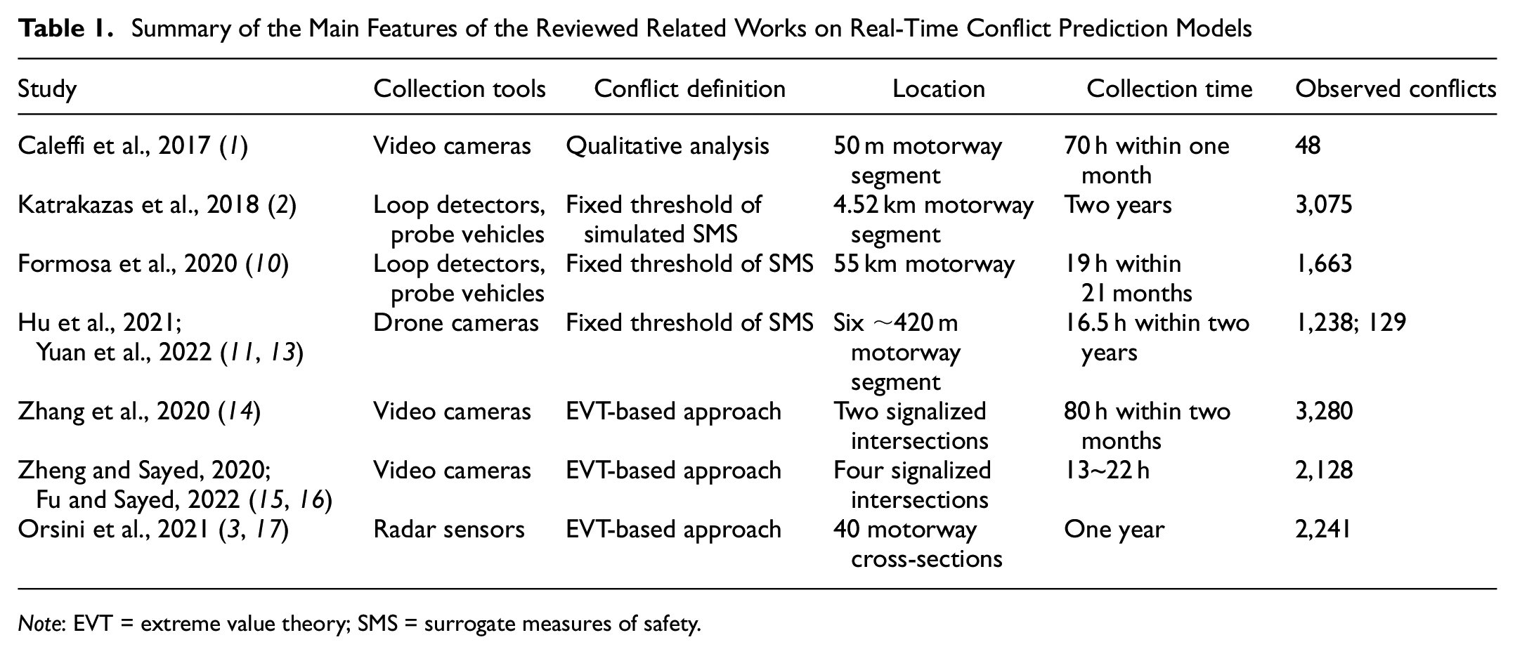
Note: EVT = extreme value theory; SMS = surrogate measures of safety.
Methodology
The development of both RTCPMs and RTConfPMs follows the same general scheme. Input traffic variables are aggregated in small time intervals, usually 5 min long ( 18 ). These records are then divided into two classes, unsafe and safe, depending on whether they are followed by a time interval that contains a crash (in the case of RTCPM) or conflicts (RTConfPM).
The two classes are strongly unbalanced, with “safe” records outnumbering “unsafe” records by several orders of magnitude. In unbalanced classification problems, models tend to classify all samples into the major class, because of their objective functions, which minimizes the sum of errors by assigning the same weight to both the major and minor classes ( 19 ). This issue is generally addressed in the RTCPM literature by resampling the dataset to obtain two balanced classes; in this work we adopted the synthetic minority oversampling technique (SMOTE), originally proposed by Chawla et al. ( 20 ). SMOTE generates synthetic samples of the minority class; these samples are points in the feature space located between neighboring original samples. SMOTE can be used in combination with random under-sampling of the majority class to obtain the desired ratio between the classes ( 20 ). It should be noted that these synthetic samples have the potential to bias the classifier if the imbalance rate is very high, and in many cases a random undrsampling of the majority class (RUMC) is recommended to obtain reliable results based exclusively on real samples ( 21 ). The choice of adopting SMOTE, consistent with Orsini et al. ( 3 ), was mainly because of the limited sample size available, which would have made RUMC unfeasible, in particular for short data collection durations. It is also worth noting that the practice of using SMOTE is becoming quite established in road safety modeling, and many recent works have applied it with good results ( 22 – 27 ).
Once a balanced training dataset is produced, a classifier is calibrated and used to make predictions. SVM is one of the most widely used machine learning classifiers in RTCPMs; it was introduced in the works of Lv et al. ( 28 ), Qu et al. ( 29 ), and Yu and Abdel-Aty ( 30 ), and has recently been applied in several others ( 31 – 33 ), sometimes in combination with SMOTE ( 22 , 34 ). The basic idea behind SVM is to find the hyperplane that separates all data points, maximizing the distance between the classes ( 35 ). If, as often happens, data from the two classes are not linearly separable, then SVM can use a soft margin, that is, a hyperplane that separates many (yet not all) data points; this is done by adding slack variables to penalize misclassification. In this work, SVM was chosen among other machine learning classifiers after carrying out a comparative study ( 17 ).
Model performance can then be evaluated using several indicators. Recall is the number of correctly predicted unsafe situations divided by the total number of observed unsafe situations. Specificity is the number of correctly predicted safe situations divided by the total number of observed safe situations. While recall is a very meaningful indicator from a safety point of view, with specificity it is possible to assess the operational feasibility of the model, since it quantifies the impact of false positives. A useful tool for an overall evaluation of the model is the receiver operating characteristic (ROC) curve, obtained by plotting the true positive rate (i.e., recall) against the false positive rate (i.e., false alarm rate, computed as 1 − specificity) at various threshold settings. From this curve it is possible to derive a widely used performance indicator, AUC, that is, the area under the ROC curve.
Data Preparation
The dataset from the present case study was previously used in Orsini et al. ( 3 , 17 ), to develop and compare several RTConfPMs and RTCPMs. Readers can find further details in those two papers.
The collection period lasted a whole year (2013) and was carried out by means of radar sensors located at 40 cross-sections of an Italian three-lane highway. For each vehicle detected on the cross-sections during this period it was possible to retrieve lane, speed, time stamp, time gap to the previous vehicle, and vehicle class (based on the detected vehicle length). These traffic data were then aggregated in 5 min intervals, providing the predictor variables described in Table 2.
Descriptive Statistics of Predictor Variables
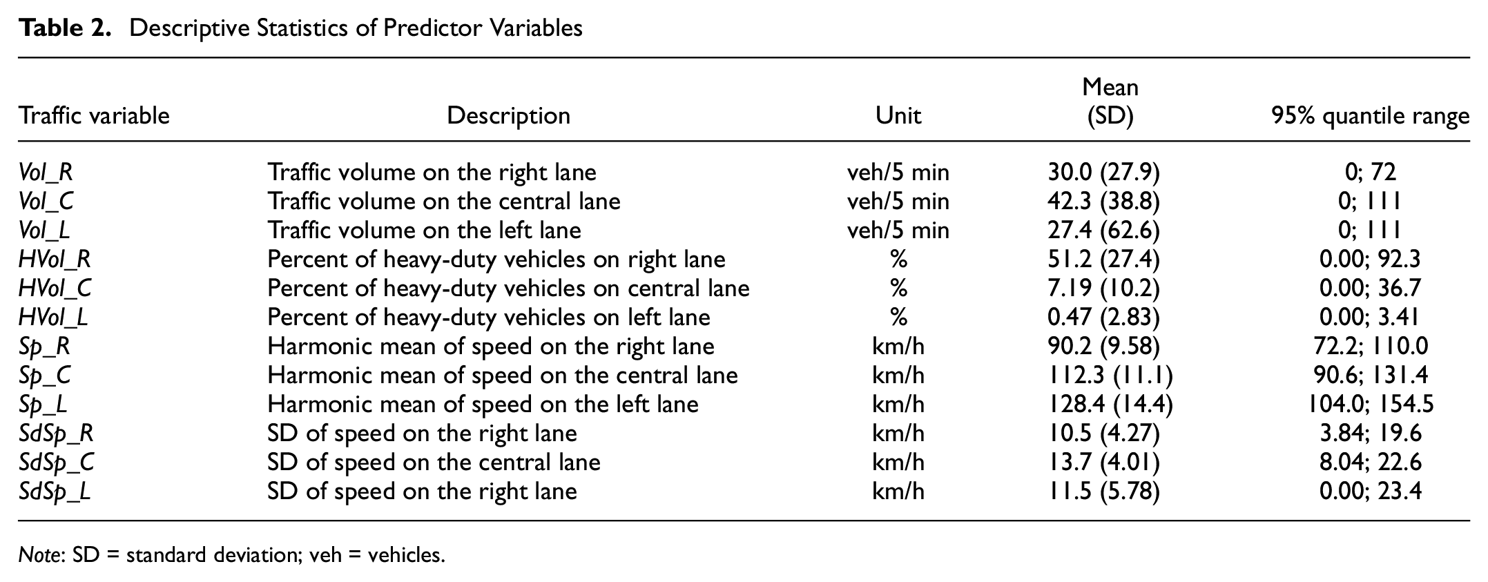
Note: SD = standard deviation; veh = vehicles.
With the same dataset it was also possible to compute a time-to-collision (TTC) for each pair of consecutive vehicles detected on the same lane:

where vL and vF are, respectively, the speed of the leading vehicle and that of the following vehicle; tGAP is the time gap between the two, recorded at the cross-section.
This SMS was then used to determine the number of conflicts detected within a given 5 min interval and whether such interval should be considered “safe” or “unsafe.” For this purpose:
Conflicts are identified by setting an appropriate TTC threshold u to separate real traffic conflicts from controlled interactions between vehicles.
A minimum number n of conflicts within the 5 min interval must be set.
TTC Threshold Selection (Parameter u)
The TTC threshold was chosen with a statistical analysis based on EVT. This theory has been applied in several road safety studies to estimate crash probabilities with SMSs ( 36 – 49 ). The procedure consists in fitting an extreme value distribution using the observed SMS, and then extrapolating a crash probability by considering crashes as “extreme” surrogate events.
In this case, observed TTC values were used to fit several generalized Pareto distributions characterized by different threshold values. Among all the fitted distributions, the best (TTC = 0.78 s) was identified with the automatic threshold selection method proposed by Thompson et al. ( 50 ) and via graphical diagnostics; the choice was then validated by comparing the estimated annual number of crashes with the observed number of crashes in a six-year time frame. More details are available in the appendix of Orsini et al. ( 3 ).
Definition of Unsafe Situations (Parameter n)
Having chosen u, it is possible to count how many conflicts were detected in each 5 min interval. The question now is: how many conflicts are enough to define a 5 min interval as unsafe? This leads to the procedure of selecting n, that is, the minimum number of conflicts within an interval required to define an interval as unsafe. This parameter n should be selected based on operational aspects and predictive performance.
From the operational aspect, as n increases, the number of intervals defined as “unsafe” decreases (Table 3); if n is too high, the number of such intervals can become even lower than that of the crashes (i.e., 88 in this case study), which is of course not desirable, since, as mentioned in the introductory section, one of the main advantages of the conflict-based approach over the crash-based is the higher number of data available for model training. On the other hand, decreasing n increases the “unsafe” intervals; however, naturally, this also tends to increase the number of alarms triggered by the model, which could become incompatible with intervention strategies.
Number of Intervals in the Full-Year Dataset Defined as “Unsafe” Depending on the Value of Parameter n
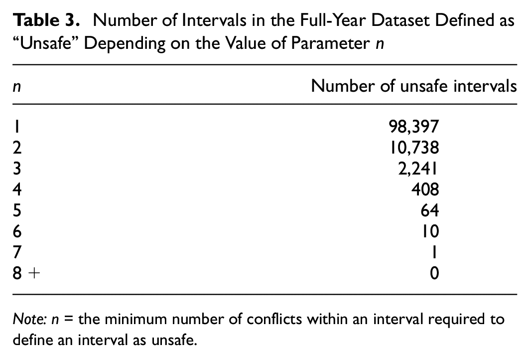
Note: n = the minimum number of conflicts within an interval required to define an interval as unsafe.
With regard to predictive performance, increasing n reduces the size of the training dataset, which could affect performance. On the contrary, reducing n tends to loosen the relationship between predictor variables and unsafe situations, which can also negatively affect performance.
In Orsini et al. ( 3 ), a sensitivity analysis of model predictive performance was carried out, considering n = 1, 2, …, 5. Figure 1 reports the results of the analysis, which identify n = 3 as the optimal value considering an observation period of one year.
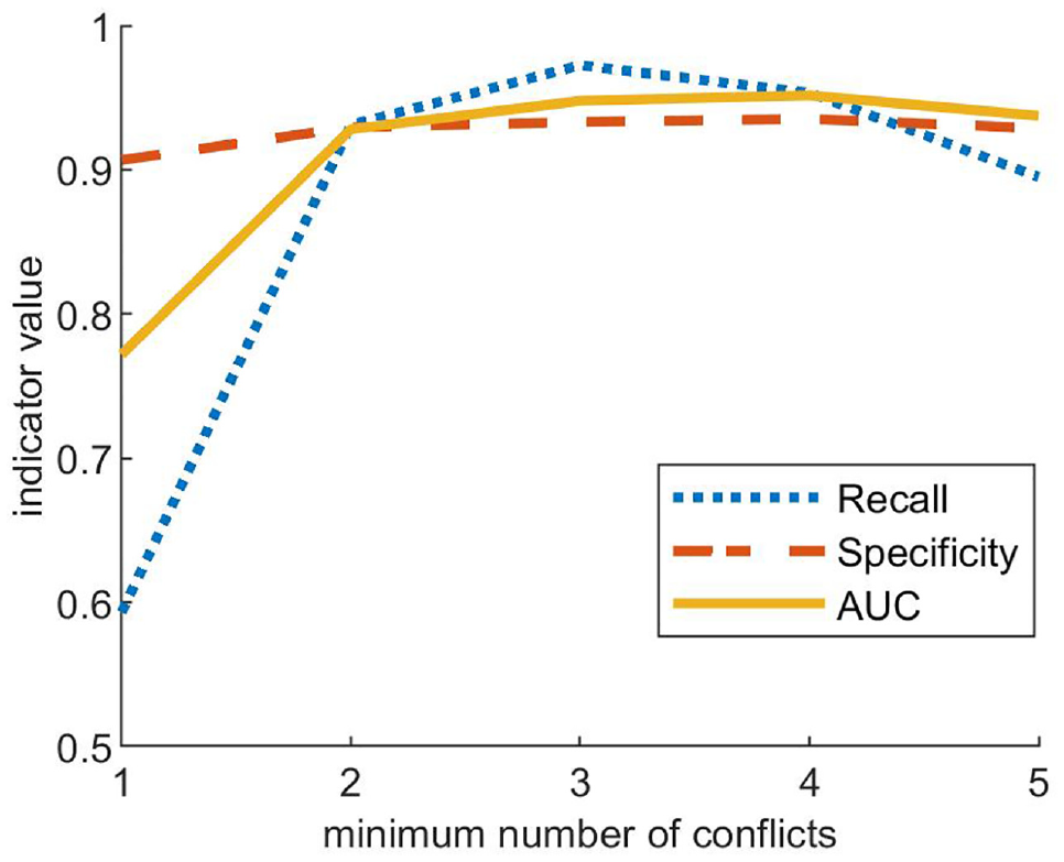
Sensitivity analysis of the effect of parameter n on performance indicator. Source: Orsini et al. ( 3 ), appendix.
However, it is relevant to highlight here that even though predictive performance is lower with n = 2, it is also true that the number of unsafe intervals observed throughout the year is almost five times higher than the case of n = 3 (see Table 3), and this may become particularly important for shorter observation times.
To sum up, with respect to the present case study, selecting a value of three for parameter n maximizes predictive performance when enough conflict data are available; on the other hand, selecting a value of two allows significantly more conflict data to be used for model calibration, given equal observation periods, at the cost of slightly lower predictive performance. For this reason, the section “Results and Discussion” will present the results of models trained considering both n = 3 and n = 2.
Results and Discussion
Sensitivity to Data Collection Duration
The analyses reported in this section aim to answer the main research question set out above, by assessing the impact of data collection time on model performance.
For this purpose, several data collection times were considered, ranging between a one-day period and a 30-day period, with one-day increments. Two sets of models were evaluated, with both n = 3 and n = 2 used to define the “unsafe” interval class; for better readability, in the remainder of the paper they will be respectively called n3 and n2 models.
For a given x-day period (x = 1, 2, …, 30), an RTConfPM was trained with only data recorded on x random days of the year and validated on data from the remaining days. The procedure to build training and test datasets is illustrated in Figure 2.
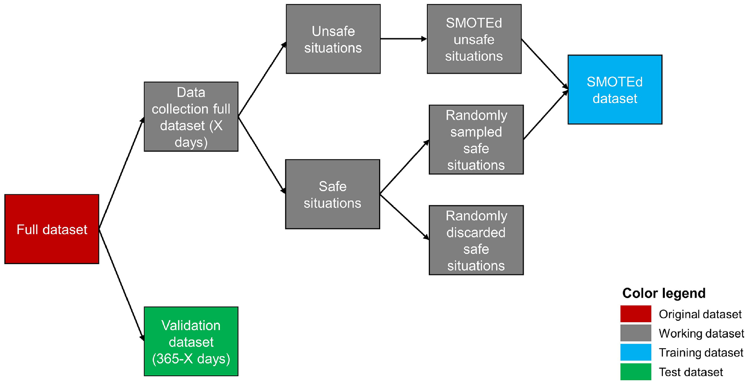
Overview of training and test dataset formation.
The x days were extracted randomly, to avoid any seasonality effect. The original full dataset was split in two, the first containing only records collected during the x days, the second containing all the remaining data. The latter dataset was set aside and used for model validation; the former was affected by a strong imbalance between the two classes, similar to the original full dataset. To deal with the unbalanced classification issue, SMOTE was applied, as have been done in many other real-time road safety applications (see “Methodology”). In practice, the data collection full dataset was split in two: the unsafe situation dataset and the safe situation dataset, each containing only records from their respective class. SMOTE (with k = 5) was applied to the unsafe situations: for each unsafe record, four other synthetic unsafe records were generated. To obtain a 1:1 ratio between unsafe and safe records, an appropriate number of records was randomly sampled from the safe situation dataset. The two sets of records were then merged in the SMOTEd dataset.
Finally, the SMOTEd (balanced) dataset was used to train the SVM and was tested on the validation dataset (which preserved real-world imbalance between classes). To account for the randomness in the selection of the x days, this procedure was repeated 100 times for each value of x.
The results are presented in Figure 3. Model performance was evaluated considering the indicator values averaged on the 100 repetitions and their 95% confidence intervals (calculated considering the 2.5 and 97.5 indicator percentiles on the 100 repetitions).
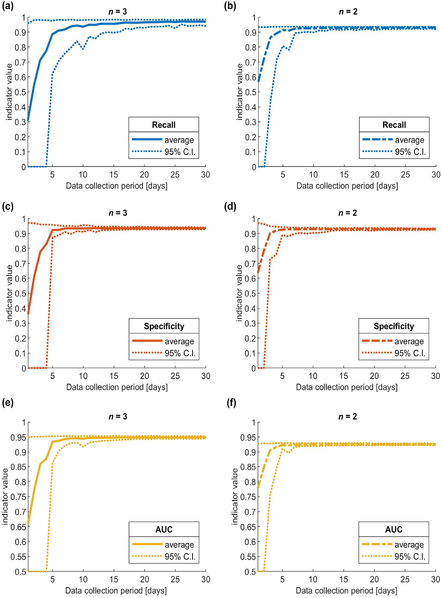
Trend of average and 95% confidence interval values, increasing data collection duration from one to 30 days, for recall, specificity, and area under the ROC curve (AUC): (a) n3 models recall, (b) n2 models recall, (c) n3 models specificity, (d) n2 models specificity, (e) n3 models AUC and (f) n2 models AUC.
For the n3 models, in all three graphs, and especially for specificity (Figure 3c) and AUC (Figure 3e), it is possible to clearly identify a sharp elbow decrease in model performance when the data collection duration is lower than five days. This shows that five or more days is a long enough data collection period to obtain performance comparable with that of a model trained on data from the whole year, with indicator values well above 0.9. Increasing the period above 10 to 15 days results in negligible improvements in specificity and AUC. Recall (Figure 3a) needs more days to stabilize, as it appears to be more influenced by randomness in the data collection period selection (its confidence interval is less narrow than those of the other indicators). Conversely, with less than five days there are not enough data to obtain reliable predictions; sometimes there were not even enough unsafe situations to calibrate the SVM (in those cases, recall and specificity were assigned a value of zero and AUC a value of 0.5).
As for the n2 models, the three graphs (Figure 3b, d , and f ) qualitatively show a similar trend, but with two important differences. First, the elbow position corresponds to a data collection period of just three days; second, when the period is longer than three days, the performance stabilizes at a slightly lower level than that of the n3 models, consistent with what was observed in the sensitivity analysis presented in the “Data Preparation” section. Figure 4 presents a direct comparison of the two sets of models, which highlights that the n2 models outperform the n3 models when the number of data collection days is less than five days; this is particularly evident in the AUC graph (Figure 4c), less so for recall and specificity (Figure 4a and b ).
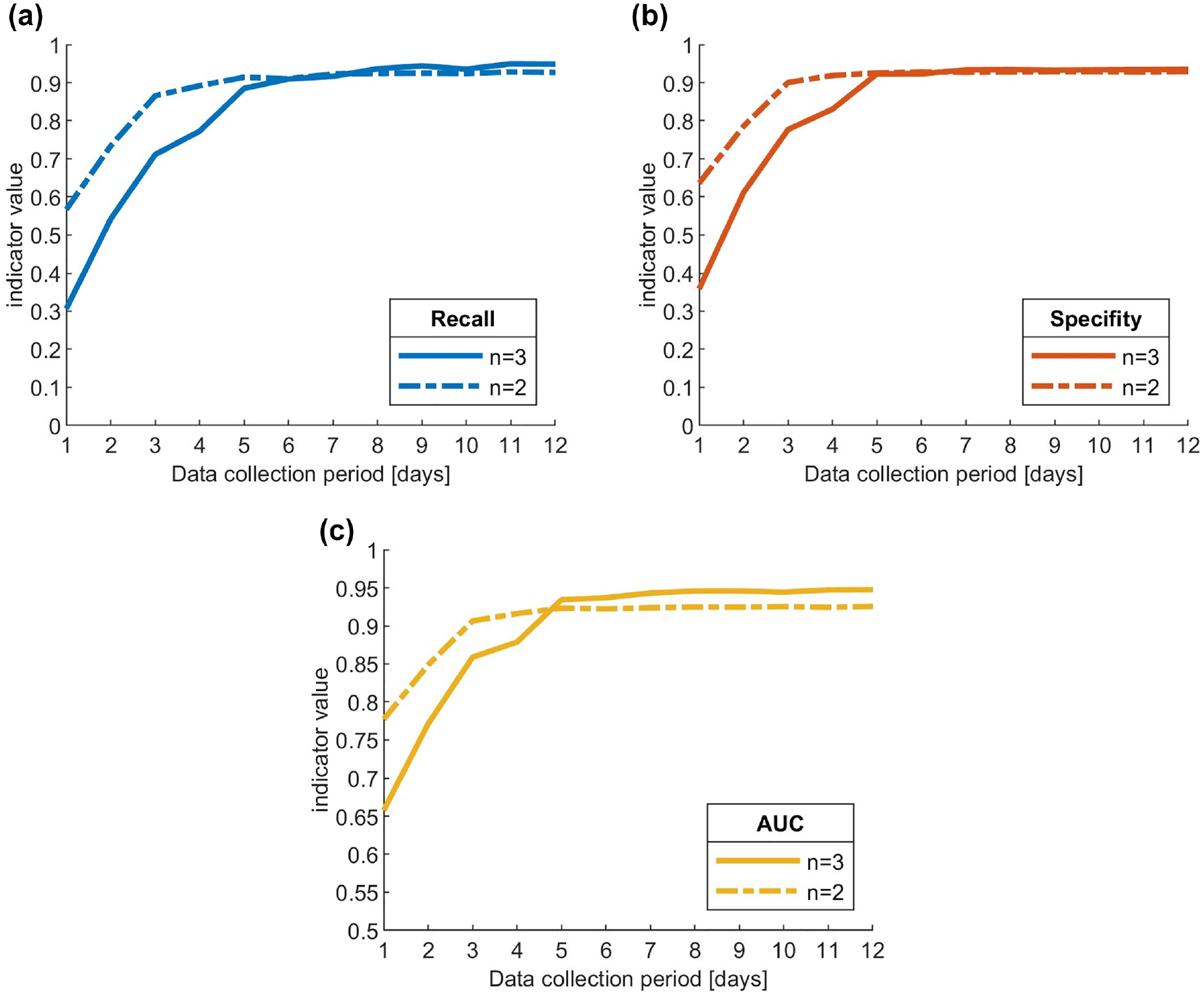
Trend comparison of average indicator values between n3 and n2 models for: (a) recall, (b) specificity, and (c) area under ROC curve (AUC).
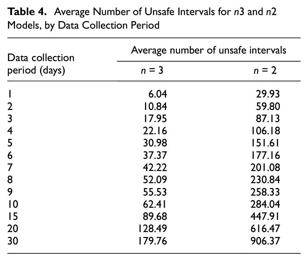
With regard to days of data collection, the results shown here are of course highly dependent on the configuration of the detectors and the traffic volumes. To compare these results with different scenarios, the reader can find in Table 4 how the number of days in this case study translates into average number of recorded unsafe 5 min intervals; for reference, in the present case study, the daily average traffic volume was around 980,000 vehicles and the total number of intervals in one day was, on average, around 9,300 (this value was not constant because malfunctions/maintenance operations meant that not all detectors were necessarily operational every day). In particular, it can be observed that the performance of n3 models stabilizes with 30 or more unsafe intervals recorded, whereas n2 models need about 90 of them. These values are much lower than the number of observed conflicts used to calibrate models in most of the previous literature (Table 1), suggesting that shorter data collection duration could have been used for such studies.
Average Number of Unsafe Intervals for n3 and n2 Models, by Data Collection Period
Robustness to Choice of Machine Learning Classifier
In general, different machine learning classifiers yield different results in predictive performance, as has been observed in several comparative works on RTConfPMs ( 2 , 14 , 17 ). Therefore, even the effects of data collection duration could be different, in principle, depending on the model used.
To assess the robustness of the findings of the present work, with respect to the machine learning classifier used, the methodological procedure reported in the previous section was replicated, testing three other machine learning classifiers: KNN, naïve Bayes (NB), and discriminant analysis (DA). These classifiers, together with SVM, were compared in a previous work of Orsini et al. ( 17 ) on the full-year dataset, which concluded that SVM and KNN were the most effective, slightly outperforming NB and DA. In that work, a decision tree was also compared, but did not provide satisfactory results because of overfitting issues, and therefore it was not included in the present analysis.
For each classifier, as in Orsini et al. ( 17 ), the best combinations of parameters were used, namely: k = 5 and Euclidean distance function for KNN, normal distribution for NB, and quadratic discriminant analysis for DA.
Figure 5 compares the trends of AUC indicator for n3 and n2 models using the three additional classifiers. It can be observed that each of the three trends is consistent with that of SVM (Figure 4c): n3 models show a constant trend when the data collection duration is longer than five days, outperforming n2 models; conversely, n2 models perform better for data collection duration of three and four days, while further reducing the period severely affects performance.
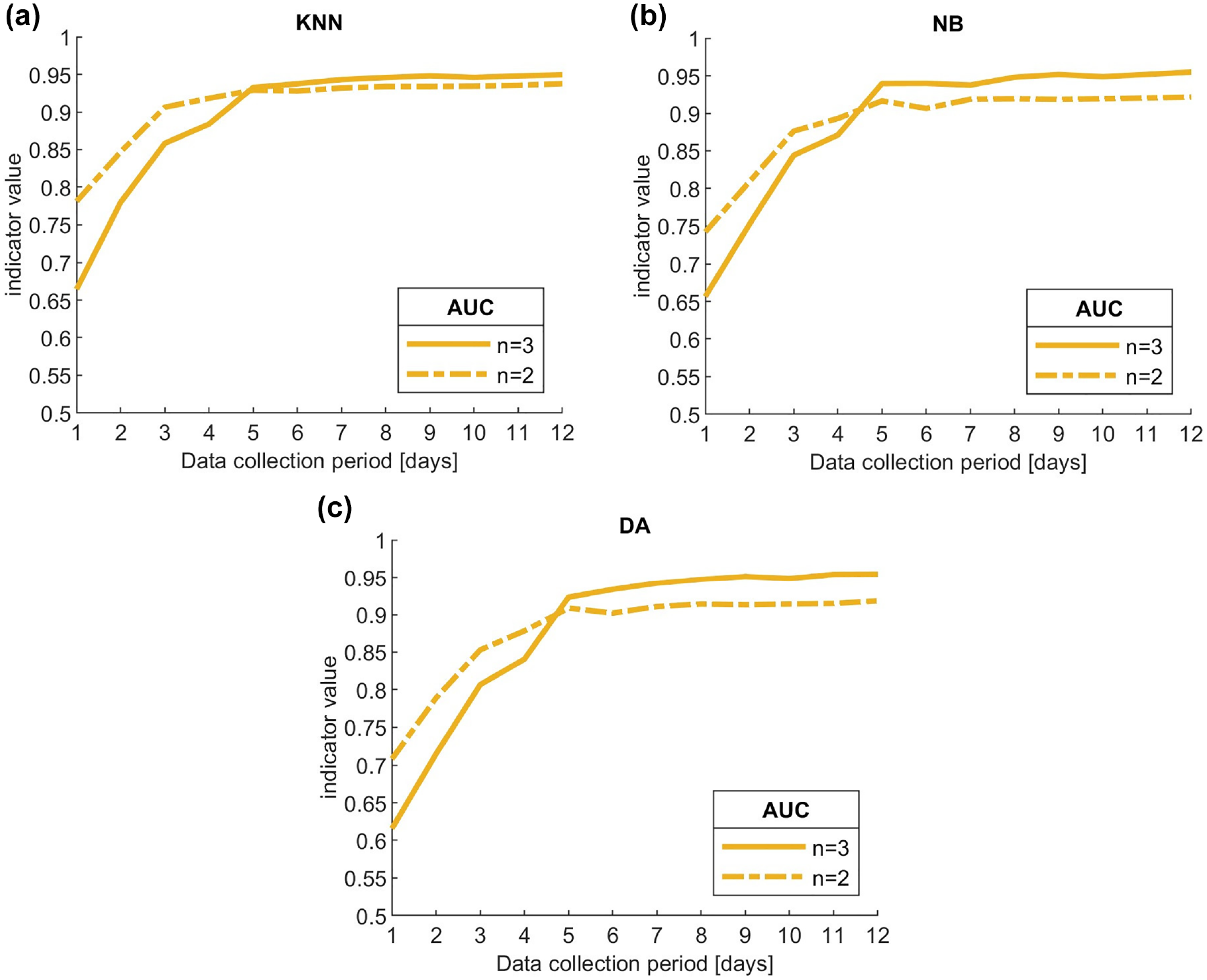
Comparison of trends in average area under the ROC curve (AUC) values between n3 and n2 models using: (a) k-nearest neighbor, (b) naïve Bayes, and (c) discriminant analysis.
This analysis shows that although using alternative machine learning classifiers can somewhat affect the results (e.g., the n2 models with NB and DA show a more relevant drop in performance than their respective n3 models, compared with SVM and KNN), the conclusions reached on the effect of data collection duration on RTConfPMs, which is the main aim of the present work, are robust with respect to the machine learning classifier chosen.
Implications for Model Resilience
In real-time road safety applications, data are collected continuously, as it is always necessary to know current traffic characteristics to predict whether there will be an unsafe situation or not in the immediate future. Therefore, the ability of an RTConfPM to be reliably calibrated with only a few days of data collection does not provide a huge practical benefit per se, as sensors must be operative all year round anyway. However, it can have significant implications for model resilience.
As mentioned in the introductory section, model resilience refers to a model’s ability to recover its predictive accuracy rapidly when faced with alterations to the predictor variables or in their interrelationships. In real-world highway applications these changes may occur in a variety of situations: prolonged lane closures for repairs, new infrastructural works (e.g., the addition of a new highway exit), sudden prolonged changes in traffic volumes for foreseeable (e.g., major events attracting people to a specific area), or unforeseeable reasons (e.g., the COVID-19 pandemic).
In such situations, a prediction model calibrated with historical data might no longer be able to provide reliable predictions. A crash-based model would need data collected for several additional months/years before being able to recover its performance, and this might not even be compatible with shorter disruptive events. Conversely, as shown in the sub-section “Sensitivity to Data Collection Duration” above, a conflict-based model would potentially need only a few days (or even hours) to adapt to the new scenario.
Similar remarks can be made considering the application of real-time road safety models for newly-built infrastructures, or infrastructure currently devoid of adequate sensors: a crash-based model would need months/years before being usable, whereas a conflict-based one would need a significantly shorter initial data collection period.
Conclusion
The present work investigated the effect of data collection time on real-time conflict prediction models to quantify its impact on predictive performance, as the existing literature did not specifically focus on this. A real-world highway case study was presented and several SVM models were trained and tested, considering different data collection times and different criteria to define the “unsafe situations” class. In particular, after a sensitivity analysis, it was determined to test models in which the minimum number of conflicts to define a 5 min interval as “unsafe” was three (i.e., n3 models), consistent with Orsini et al. ( 3 ), but also to test another set of models reducing this number to two (i.e., n2 models).
With respect to the main research question (i.e., how does data collection duration affect RTConfPMs performance?), in the specific case study analyzed, n3 models were able to provide reliable results with just five days of data collection, whereas longer collection times were able to only marginally improve predictive performance, and the improvement was virtually nonexistent for collection periods of more than 15 days. With n2 models, it was possible to reduce the collection period to just three days, while maintaining acceptable predictive performance. For collection times longer than five days, however, they were slightly outperformed by the n3 models, because of the weaker relationship between the predictor traffic variables and the response variable. Although this duration of data collection is closely related to the particular case study analyzed, the findings can be more generally extended by considering the number of recorded unsafe situations: for example, with a five-day collection period, n3 models were trained on average with about 30 unsafe situations; with a three-day collection period, n2 models were trained on average with about 90 unsafe situations. By comparing these values with the number of observed conflicts used to calibrate RTConfPMs in previous literature (Table 1), our findings suggest that several works could have used even significantly shorter data collection durations, further highlighting one of the advantages of the conflict-based approach over the crash-based, which requires shorter time to collect data.
This work provides several novel and relevant takeaways for both practical and scientific applications, since, as mentioned in “Related Works,” previous literature dealt with several fundamental research and practical issues, yet without expressly investigating and quantifying the sensitivity of RTConfPMs to the data collection duration. As extensively discussed in the paper, this has significant implications for model resilience: contrary to traditional real-time crash prediction models, these conflict-based models are potentially able to adapt themselves to changes in the characteristics of the response variables or of the infrastructure itself. A resilient real-time road safety prediction model is of great interest for road authorities, as it is functional for an effective implementation of intervention strategies, which should be affected as little as possible by changes in traffic and road characteristics.
These findings highlight the relevance of real-time conflict prediction models as a more flexible alternative to the crash-based approach, and that this flexibility can be fine-tuned by appropriately defining the criteria used to identify the “unsafe situation” class, which can be done with the aim of either prioritizing model performance or resilience.
The main limitation of the present study is that the analyses were carried out exclusively on cross-sectional highway data. Future research will involve the replication of the current study considering different collection methods (e.g., probe vehicles), alternative predictive models (e.g., neural networks), and different contexts (e.g., urban intersections), with the ultimate goal of further generalizing the findings on the impacts of data collection duration on RTConfPMs.
Footnotes
Author Contributions
The authors confirm contribution to the paper as follows: study conception and design: F. Orsini, M. Gastaldi, R. Rossi; data elaboration: F. Orsini; analysis and interpretation of results: F. Orsini, M. Gastaldi, R. Rossi; draft manuscript preparation: F. Orsini. All authors reviewed the results and approved the final version of the manuscript.
Declaration of Conflicting Interests
The author(s) declared no potential conflicts of interest with respect to the research, authorship, and/or publication of this article.
Funding
The author(s) disclosed receipt of the following financial support for the research, authorship, and/or publication of this article: This work was supported by the University of Padua (“Advances in proactive and reactive approaches to road safety: development of innovative crash risk prediction and automatic incident detection systems,” BIRD177377/17).
Data Availability Statement
The datasets analyzed during the current study are available from the corresponding author on reasonable request.