Forecasting Traffic Speed during Daytime from Google Street View Images using Deep Learning

Abstract

Traffic forecasting plays an important role in urban planning. Deep learning methods outperform traditional traffic flow forecasting models because of their ability to capture spatiotemporal characteristics of traffic conditions. However, these methods require high-quality historical traffic data, which can be both difficult to acquire and non-comprehensive, making it hard to predict traffic flows at the city scale. To resolve this problem, we implemented a deep learning method, SceneGCN, to forecast traffic speed at the city scale. The model involves two steps: firstly, scene features are extracted from Google Street View (GSV) images for each road segment using pretrained Resnet18 models. Then, the extracted features are entered into a graph convolutional neural network to predict traffic speed at different hours of the day. Our results show that the accuracy of the model can reach up to 86.5% and the Resnet18 model pretrained by Places365 is the best choice to extract scene features for traffic forecasting tasks. Finally, we conclude that the proposed model can predict traffic speed efficiently at the city scale and GSV images have the potential to capture information about human activities.

In the process of urban expansion, populations can rapidly increase in areas disconnected from places of work, resources, and leisure, leading to problems such as traffic congestion, crashes, and air pollution. The ability to forecast traffic, therefore, is vital to the success of traffic control, traffic safety improvements, and CO2 emission reductions. Traditionally, traffic forecasting relies on data-driven approaches, such as the autoregressive integrated moving average (ARIMA) model, linear regression models, and theory-driven traffic simulation models, such as the queuing theory model ( 1 – 6 ). However, these methods all assume that the traffic operates under ideal conditions, making them inefficient in a large-scale transportation system analysis with massive real-time data.

The development of machine learning provides us new approaches to capture more complex information from existing traffic datasets. These approaches—known as nonparametric methods—such as k-nearest neighbor (KNN), Bayesian network, and support vector machine (SVM) have been successfully applied in previous traffic prediction research ( 7 – 9 ). Recently, deep learning, an advanced type of machine learning, outperformed traditional parametric as well as non-parametric machine learning approaches in traffic prediction accuracy ( 10 ). Non-deep-learning methods perform well in capturing the temporal dependency of traffic flow; however, they are not able to take spatial information into account, which is another vital factor which influences the accuracy of traffic forecasting.

To address this problem, graph neural networks (GNN) are integrated with deep learning models. Different kinds of recurrent neural networks (RNN), such as long short-term memory (LSTM) and gated recurrent unit (GRU), are used in these models to glean temporal information from historical traffic data. GNN are employed to integrate the spatial features of nodes in road networks. Examples include the highly performed T-GCN, DST-GCNN, STGNN, GaAN, and so on ( 11 – 14 ). Even though these models reach a high level of accuracy for traffic flow prediction, there are two problems that still need to be solved. Firstly, these models cannot capture the physical characteristics of roads such as number of lanes and road condition. The function of surrounding areas, which cannot be learned by existing RNN and GNN models, is another significant factor that may influence the traffic flow and the relationship between connected roads. Secondly, these models are trained based on high-quality historic traffic data collected from specific roads equipped with traffic sensors, which makes it difficult to predict the traffic condition at city scale.

For these two problems, Google Street View (GSV) images have the potential to capture the road conditions and the information of functions of its surrounding area. The development of convolutional neural networks (CNN), such as VGG, ResNet, YOLO, and Mask RCNN, provide efficient approaches to extract scene features from GSV images ( 15 , 16 ). These scene features include: urban functions, urban built environment, place characteristics, and so forth ( 17 – 19 ). Additionally, GSV images can serve as a supplement to existing historical traffic data to predict traffic flow at the city scale. With these scene features, it is possible to predict hourly traffic flows for streets without historical data.

To address the challenges of existing integrated GNN and RNN models and to prove the ability of scene features extracted from GSV images to predict traffic flow, in this paper we propose a framework to predict traffic flow hourly from GSV images by combining CNN and GNN. A CNN framework will be used to extract scene features from GSV images for each street and these features will be input to a GNN to capture the spatial information of the road network.

Literature Review

Traffic forecasting methods can be divided into two categories: parametric and nonparametric. Parametric methods construct the model structure based on certain theoretical assumptions with parameters calculated based on empirical data ( 20 ). Nonparametric methods, also known as data-driven methods, involve a more complex model structure that can be trained without prior knowledge or theoretical assumptions.

Parametric Approaches

Examples of parametric approaches for traffic forecasting include the autoregressive integrated moving average (ARIMA) model, the linear regression model, and the Kalman filter model (1–5, 21 ). ARIMA—also written as ARIMA(b, d, q)—is one of the most widely used models to forecast traffic flow. The autoregressive, integrated, and moving average polynomial orders are essential parameters used to build the ARIMA time series model ( 22 , 23 ). However, since traffic conditions are neither stationary nor linear, parametric approaches are not applicable to the rapid changes in traffic flow.

Nonparametric Methods

Nonparametric approaches such as KNN, Bayesian network, SVM, and artificial neural networks can successfully capture the complex and nonlinear characteristics of traffic flow ( 8 , 24 ). The KNN method requires a high-quality traffic flow database. This method searches for data that are similar to observed data at certain locations, such as a station, then similar traffic flow series are used to forecast the traffic flow of the station ( 7 , 25 ). Zhang et al. present a KNN model to predict urban expressway flow with up to 90% accuracy ( 26 ). The SVM method involves mapping data to a high-dimensional feature space and performing linear regressions within that space ( 27 ). Ling et al. introduced a multi-kernel SVM (MSVM) to predict traffic flow, and a novel adaptive particle swarm optimization (APSO) algorithm to optimize the parameters of MSVM. Their results show that this algorithm can make timely and adaptive predictions during peak hour when the traffic conditions change rapidly ( 28 ).

Nonparametric models can also be integrated with other nonparametric models to improve overall performance. Ahn et al. used both support vector regression and Bayesian classifiers to conduct real-time traffic flow prediction ( 29 ). Random forest and support vector regression are integrated to perform short-term traffic flow forecasting ( 30 ). Additionally, the combination of Kalman filtering and KNN, KNN and SVM, KNN and LSTM, KNN and neural networks, and so forth, are performed to predict short-term traffic flow ( 31 – 34 ).

With the rapid development of deep learning, deep neural network models are now widely used to forecast traffic flow ( 35 – 41 ). At present, modeling methods based on deep neural networks achieve the most accurate results because of their ability to extract dynamic traffic features. These methods can identify traffic features without prior knowledge or assumptions, handle multi-dimensional data and flexible model structures, and employ strong generalization and learning abilities ( 11 , 20 , 35 ). In recent years, RNNs and their variants, LSTM and GRU, have received attention because of their self-circulation mechanism, which allows them to learn temporal dependence, and their ability to outperform other types of deep neural networks ( 11 ).Tian and Pan proposed an LSTM model to determine optimal time lags dynamically. Their results show that LSTM achieves higher accuracy than other methods including random walk (RW), SVM, single-layer feed forward neural network (FFNN) and stacked autoencoder (SAE) ( 42 ). However, these models only focus on temporal characteristics, meaning they cannot capture the spatial dependencies of traffic flow. GNN can aggregate and transform traffic information through edges in road networks ( 43 – 45 ). This allows GNN to capture the spatial dependencies of traffic flow, which improves the accuracy of traffic forecasting. More and more researchers have combined these deep learning models with GNN to capture the spatiotemporal characteristics of traffic flow. Wu et al. proposed a graph attention LSTM network (GAN-LSTM) to capture spatiotemporal correlations for traffic flow forecasting, and found GAN-LSTM outperformed other multi-link traffic flow forecasting models: diffusion convolutional recurrent neural network (DCRNN), LSTM, and feed forward neural network (FNN)( 46 ). A gated CNN can be combined with a graph convolutional network (GCN) to form a spatio-temporal GCN (STGCN), which captures comprehensive spatiotemporal correlations and runs much faster with fewer parameters ( 13 ). Zhang et al. proposed a model based on gated attention networks (GaAN) to extract spatiotemporal characteristics of traffic flow ( 14 ). The combination of RNN and GNN requires both a historical dataset to train the model and observation traffic flow data to forecast traffic conditions. CNN and RNN can also be combined to capture the spatiotemporal characteristics of traffic flow at the city scale ( 47 , 48 ). This method involves transforming the road network to raster maps, with the values of each cell representing the condition of traffic, then typical RNN networks are used to capture the temporal characteristics of traffic data for each cell. With these models, we can learn the spatiotemporal features of traffic flow data at the city level; however, these models require traffic data on all the streets, such as trajectory data, which limits this approach to situations where a city-wide dataset is accessible. The need for both historical and observation data makes these models difficult to apply to the entire city.

Methodology

Problem Definition

In the problem of traffic forecasting, we intend to predict hourly traffic speeds during workdays based on scene features extracted from GSV images. Specifically, the scene features of each road are represented on a traffic network model. We describe the traffic network as an unweighted graph $G=(V,E)$ , where $V=\{v_1,v_2,...,v_N\}$ is a set of road nodes (we treat each road as a node), N is the number of the nodes, and E is a set of edges representing the connection of each road.

The adjacency matrix, $A\in \left\{R^{N\times N}\right\}$ , can also represent the connection between roads. For each element in the adjacency matrix, $A_{\mathrm{ij}}$ , which represents the connection between node i and node j, there are only two possible values (0 means no connection; 1 means they are connected). The scene features extracted from GSV images for road nodes can be represented as a feature matrix, $X\in X^{N\times D}$ , in which $X_i=[x_1,x_2,...,x_D]$ represents features of node i, where D represents the dimension of scene features for each node.

The hourly traffic speed information for each node can be represented as a sequence $y=(Y_1,Y_2,...,Y_{24})$ on the traffic network, where each $Y_t$ is the traffic speed at time t.

Thus, the problem of traffic speed forecasting can be defined as building a model $f$ on the traffic network G and feature matrix $X_i=[x_1,x_2,...,x_D]$ to predict the hourly traffic speed $y=(Y_1,Y_2,...,Y_{24})$ , which is shown as (1):

$$(Y_1,Y_2,\dots ,Y_{24})=f(G;[x_1,x_2,\dots ,x_D])$$

(1)

where

D = the dimension of extracted scene features for each street node.

Method

The proposed scene graph CNN framework consists of two parts: the CNN and the GNN. As shown in Figure 1, we first use a pretrained CNN model, Resnet18, to extract scene features from GSV images for each street node, then the average of these features is calculated to construct the feature matrix X. Secondly, the generated scene features are entered into a GCN to capture the spatial dependency. Finally, we get a predicted hourly traffic speed sequence, $\hat{y}=({\hat{Y}}_1,{\hat{Y}}_2,...,{\hat{Y}}_{24})$ , for each road node, where each ${\hat{Y}}_t$ represents the traffic speed at time t.

Figure 1.

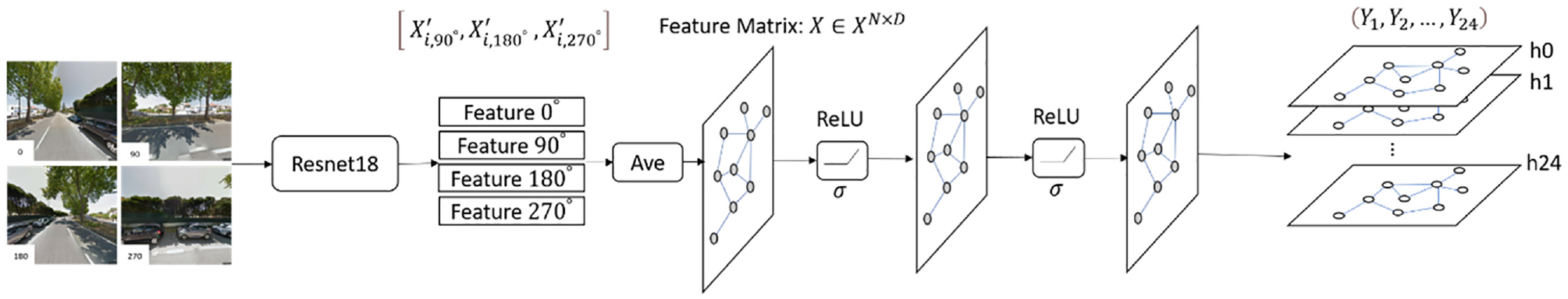
Structure of scene graph convolutional network (GCN).

Scene Features Extraction

Four GSV images at heading angles of 0°, 90°, 180°, and 270° for each street node are generated using the GSV static API. For each node, we use Resnet18 to extract scene features from GSV. Features in all heading angles are generated, ${\mathit{X}}_{\mathit{i}}^{\text{'}}=[{\mathit{X}}_{\mathit{i},90\mathbf{°}}^{\text{'}},{\mathit{X}}_{\mathit{i},180\mathbf{°}}^{\text{'}},{\mathit{X}}_{\mathit{i},270\mathbf{°}}^{\text{'}}]$ , where ${\mathit{X}}_{\mathit{i}}^{\text{'}}$ is the list of features at each of the four heading angles of node i. Then, the average value of each location is calculated, ${\mathit{X}}_{\mathit{i},\mathit{j}}=\frac{1}{4}({\mathit{X}}_{\mathit{i},0\mathbf{°},\mathit{j}}^{\text{'}}+{\mathit{X}}_{\mathit{i},90\mathbf{°},\mathit{j}}^{\text{'}}+{\mathit{X}}_{\mathit{i},180\mathbf{°},\mathit{j}}^{\text{'}}+{\mathit{X}}_{\mathit{i},270\mathbf{°},\mathit{j}}^{\text{'}})$ , where ${\mathit{X}}_{\mathit{i},\mathit{j}}$ is the feature of node i at dimension j, and $\mathit{i}\in \mathit{N},\mathit{j}\in \mathit{D}$ . We use a pretrained Resnet18 to extract scene features. The model is trained by the Places365 dataset with a high top-5 accuracy of 85.07% ( 49 ). It employs an identity shortcut connection mechanism to skip one or more layers when training the model, so that more layers could be included in the model resulting in higher accuracy. Resnet18 requires relatively fewer parameters and less computational cost to extract features from images than other methods. The structure of our Resnet is shown as Figure 2.

Figure 2.

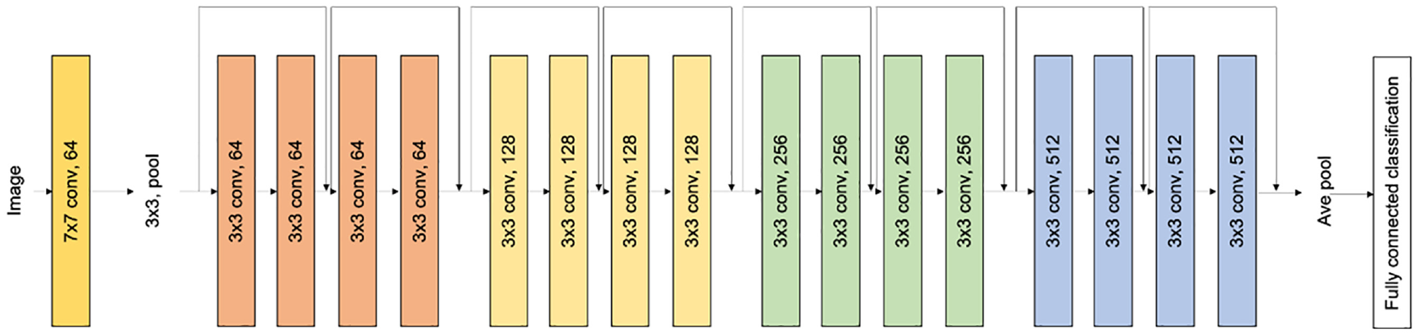
Structure of Resnet18.

Spatial Dependence Modeling

The traffic speed in a street node is influenced not only by its own features, but also by the other street nodes connected to it. GCN has been successfully used in extracting spatial dependencies of traffic networks to predict traffic flow with high accuracy. The mechanism of GCN is to construct a filter in the Fourier domain based on adjacency matrix $A$ and feature matrix $X$ . For each street node, the filter will aggregate the features of its connected nodes, then several convolutional layers are stacked to extract further and more complex spatial features. The GCN can be expressed as:

$$X^{(l+1)}=\sigma \left({\tilde{D}}^{-\frac{1}{2}}\hat{A}{\tilde{D}}^{-\frac{1}{2}}{X}^l{W}^l\right)$$

(2)

where

$\hat{A}=A+I_N$ = the adjacent matrix with self-connections,

$I_N$ = the identity matrix,

$\tilde{D}=\sum _j{\hat{A}}_{\mathrm{ij}}$ , $\tilde{D}$ = the degree matrix,

$X^l$ = the output feature matrix of layer $l$ ,

$W^l$ = the trainable weights of layer $l$ , and

$\sigma (.)$ = the activation function (ReLU).

In this research, we adopt a two-layer GCN to extract spatial features from the traffic network. The process can be expressed as:

$$\hat{y}=\tilde{A}\sigma \left(\tilde{A}{X}_0{W}_0\right)W_1$$

(3)

where

$\hat{y}\in R^{N\times 24}$ = the predicted hourly traffic speed,

$\tilde{A}={\tilde{D}}^{-\frac{1}{2}}\hat{A}{\tilde{D}}^{-\frac{1}{2}}$ , $X_0\in R^{N\times D}$ = the scene features extracted from GSV, and

$W_0\in R^{D\times T}$ = trainable weight matrix from the hidden to the output layer, and

$W_1\in R^{T\times 24}$ = trainable weight matrix from the hidden to the output layer.

Experiments

In this section, we set up experiments to evaluate the performance of our proposed SceneGCN framework. We first introduce the dataset used for training our model and evaluation metrics. Then, different CNN models are employed to extract scene features. Finally, we present the experiment results and interpretation of our proposed model.

Data Description

Taxi Trajectory Dataset

The performance of the proposed SceneGCN model is evaluated on a taxi trajectory dataset collected in the city of Porto, Portugal ( 50 ). A total of 442 taxis were equipped with mobile data terminals to collect trajectory data for a complete year (from July 1, 2013, to June 30, 2014). In this dataset, GPS signals are collected every 15 s and timestamps of the start point for each trip are recorded. We select Monday to Friday (except holidays or other special days and days before these days) to prepare our training and testing dataset.

Google Street View Imagery (GSV)

GSV provides us 360° panoramic scenes along streets at the same viewing angles as pedestrians. It provides a huge amount of imagery to explore urban built environments. The Google Cloud platform provides us a GSV static API to download these images automatically. The necessary parameters include location (latitude and longitude of the images), pano-ID (the specific panorama ID), output size of each image, and key of the API, as well as other optional parameters, such as the heading (compass heading of the camera), fov (horizontal field of view of the image) and pitch (the up and down angle of the camera relative to the GSV vehicle). In this research, we download GSV images for each road segment at the central point of each road at heading angles 0°, 90°, 180°, and 270°. Finally, 18,324 images are downloaded to gather scene features for each road segment. These images are used to extract scene features, which are possibilities of different scene types, such as apartments, highways, bridges, parking lots, and so forth. Since these features are extracted from a pretrained Resnet model with a high accuracy, the time the images are captured will not influence the extraction of the feature ( 49 ). To match the time of the images and taxi dataset, we downloaded the GSV images from year 2013 to 2014. Figure 3 shows examples of our downloaded images.

Figure 3.

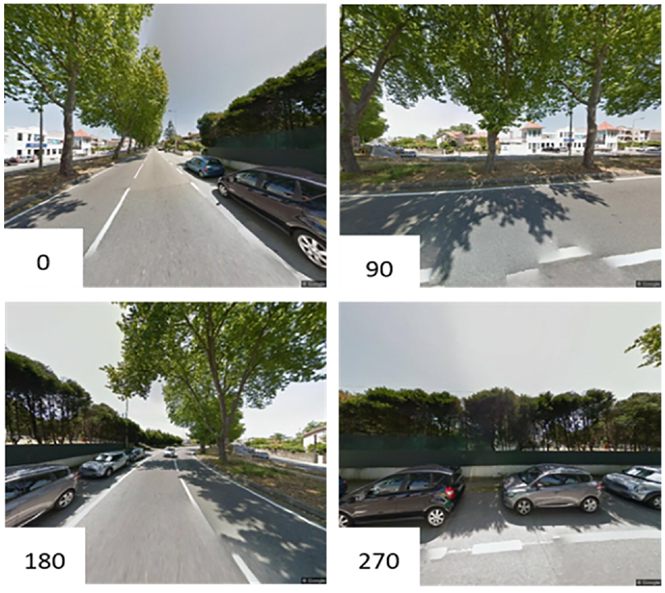
Examples of downloaded Google Street View at heading angles of 0° (top left), 90° (top right), 180° (bottom left), and 270° (bottom right).

Evaluation Metrics

To evaluate the performance of the SceneGCN, we use three metrics:

• 1) Mean absolute error (MAE):

$$\mathit{MAE}=\frac{1}{\mathit{n}}\sum _{\mathit{i}=1}^{\mathit{n}}|{\mathit{f}}_{\mathit{i}}-\widehat{{\mathit{f}}_{\mathit{i}}}|$$

(4)

• 2) Root mean squared error (RMSE):

$$\mathit{RMSE}={\left[\frac{1}{\mathit{n}}\sum _{\mathit{i}=1}^{\mathit{n}}{\left(|{\mathit{f}}_{\mathit{i}}-{\hat{\mathit{f}}}_{\mathit{i}}|\right)}^2\right]}^{\frac{1}{2}}$$

(5)

• 3) Mean absolute percentage error (MAPE):

$$\mathit{MAE}=\frac{1}{\mathit{n}}\sum _{\mathit{i}=1}^{\mathit{n}}\frac{|{\mathit{f}}_{\mathit{i}}-{\hat{\mathit{f}}}_{\mathit{i}}|}{\mathit{n}}$$

(6)

where

${\mathit{f}}_{\mathit{i}}$ = the real traffic speed, and

${\hat{\mathit{f}}}_{\mathit{i}}$ = the predicted traffic speed.

Model Parameters

Our proposed model deals with two tasks: scene feature extraction from GSV using CNN, and traffic speed prediction based on GCN. For scene feature extraction, we adopt two Resnet18 models pretrained by two different datasets:

• Places365: The Places365 dataset classifies images into 365 categories of scenes, such as highway, forest, field, street, church, plaza, and so on ( 51 ). The weights of the model are trained by 18 million images and predicts the category of each image with high accuracy ( 49 ).

• ImageNet: The ImageNet dataset classifies images into 1,000 object categories, including different kinds of cars, animals, vegetation, infrastructure, and so on.

Places365 aims to recognize scene features at a larger, more general scale, while ImageNet focuses on specific objects. We compared the performance of these two pretrained models on traffic speed forecasting to determine the most suitable prediction model. In each pretrained model, we keep the pretrained weights, and test whether containing the classification layer will influence the performance of our model.

In total, four experiments are conducted to evaluate the performance of our proposed model: Resnet18 pretrained by Places365 containing the classification layer, which generates a 365 dimension set of features for each road node; Resnet18 pretrained by Places365 without classification layer, which generates a 512 dimension set of features for each road node; Resnet18 pretrained by ImageNet containing the last classification layer and without the last classification layer, which obtains a 1,000 dimension set and 512 dimension set of features for each road node, respectively. For each experiment, the generated features are entered into a two-layer GCN to predict traffic speed. Finally, we use the MAE as the loss function (L1Loss) to reduce the error between predicted speed and real speed during the training process. The loss function is defined as:

$$\mathrm{loss}=\frac{1}{n}\sum _i^n|\widehat{y_i}-y_i|$$

(7)

where

$n$ = the number of predicted values,

${\hat{y}}_i$ = the predicted traffic speed value, and

$y_i$ = the real traffic speed value.

Experimental Results

We first processed the taxi trajectory dataset, then we obtained the training dataset, validation dataset, and test dataset with sizes of 600, 300, and 303, respectively. Scene features were extracted and entered into the GCN to train the model. The most accurate result for each experiment was generated after training about 2,500 epochs. We used the test dataset to evaluate our model. The performance of our models is shown in Table 1. From the evaluation matrix we find that the GCN trained by features extracted by the Places365 pretrained model has MAPE, RMSE, and MAE of around 0.35, 15.9, and 14.5 respectively, which are lower than that of the ImageNet pretrained models, which are around 0.37, 17.02, and 15.6, respectively. The classification layer has little effect on performance of our proposed model. A total of 365 scenes features obtained by Resnet18 with classification layer predict the traffic speed at similar errors as 512 scenes features extracted by Resnet18 without classification layer. Traffic speeds predicted by 365 scene features are more stable than that predicted by 512 features. So, we chose the 363 scene features extracted by Resnet18 (with classification layer, and pretrained by Places365) as our feature matrix to train the GCN model.

Table 1.

Evaluation Matrix

Model		MAPE	RMSE	MAE
Places365	365 scenes	0.348	15.91	14.55
	512 features	0.347	15.87	14.47
ImageNet	1,000 classes	0.377	17.02	15.64
	512 features	0.375	17.02	15.67

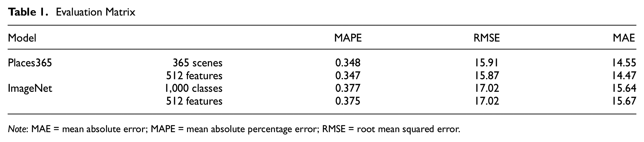
Note: MAE = mean absolute error; MAPE = mean absolute percentage error; RMSE = root mean squared error.

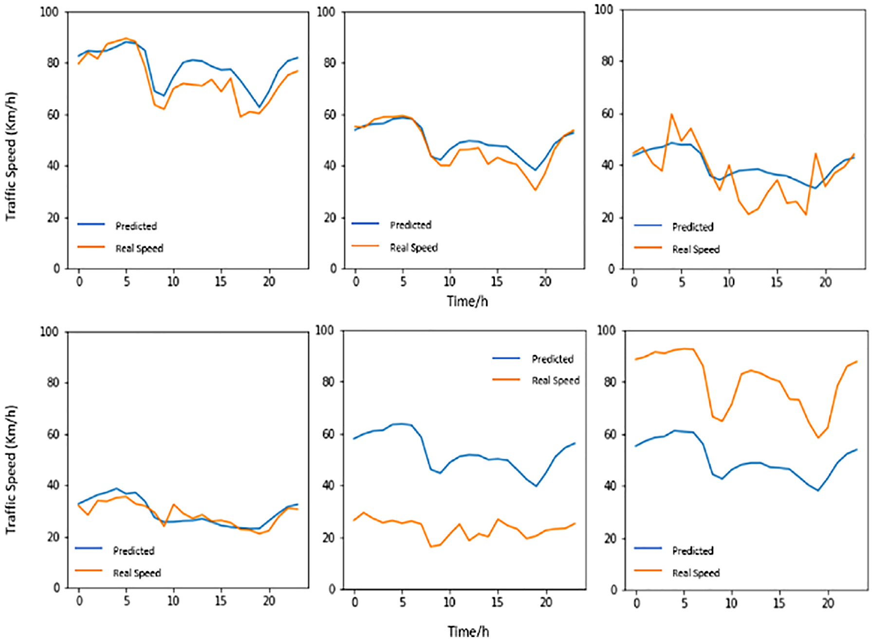
Figure 4 shows a selection of the results of our test dataset. We can see that our proposed model can predict traffic speed patterns during the workday with high accuracy. The predicted results in these figures show that, overall, traffic speeds in the city of Porto experience two rapid declines from 6 a.m. to 9 a.m. and 4 p.m. to 7 p.m. The lowest speeds occur at 8 a.m. and between 6 p.m. and 7 pm. After these valley hours, traffic speeds will recover to normal speed within one or two hours. The traffic speeds at night (from 10 p.m. to 5 a.m.) are faster than during daytime. The model can predict traffic speeds ranging from 0 km/h to 100 km/h with a high degree of accuracy. However, some road nodes are overestimated or underestimated. Table 2 shows that, in our test dataset, 17 road nodes are overestimated, 24 road nodes are underestimated, and 262 road nodes are predicted correctly. More detailed reasons on prediction errors are analyzed in the following paragraph.

Figure 4.

Result of test data.

Table 2.

Accuracy of SceneGCN

	Count	Percentage
Overestimate	17	5.6%
Underestimate	24	7.9%
Correct	262	86.5%

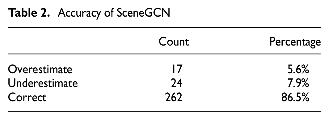
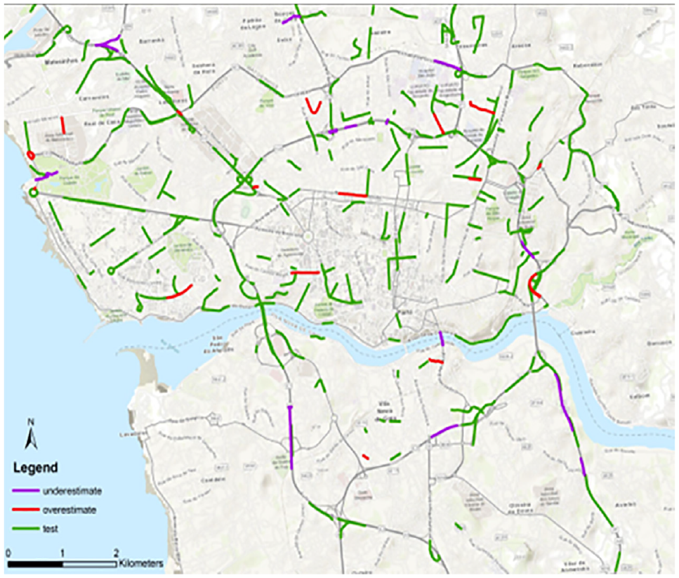
Figure 5 shows the result map of our test dataset. Purple lines are road nodes that are underestimated, red lines are road nodes that are overestimated, and green lines are road nodes that are predicted correctly. From this map we can identify that the road nodes that are underestimated are mainly located at the entrance and exit of highways. This is because these road nodes connect high-speed roads to roads with low speeds, which will be aggregated and result in an underestimated speed prediction through GCN. Also, the speeds at the entrances and exits of highways are usually lower than those on normal highway nodes. For overestimated road nodes, they are mainly located near highways. This is because some highway nodes capture features of surrounding buildings, which can cause errors that confuse these nodes with other streets with similar building scenes. Also, some overestimated roads are connected to highways, therefore information from these highways will be transferred to these overestimated roads through the GCN.

Figure 5.

Result map of test dataset.

Finally, we forecasted traffic speeds for each hour of the day for the city of Porto. Figure 6 shows predicted traffic speeds at the city scale (taken at 6 a.m., noon, 6 p.m., and midnight.). The map shows that, spatially, the traffic speed of highways is much higher than that of city roads. Traffic speed is lowest at the center of the city. Temporally, traffic speed is higher at night than at any other time, and traffic speed is lowest during commuting hours (6 p.m. in this map). The red lines in Figure 6 have the lowest traffic speed, revealing areas of traffic congestion.

Figure 6.

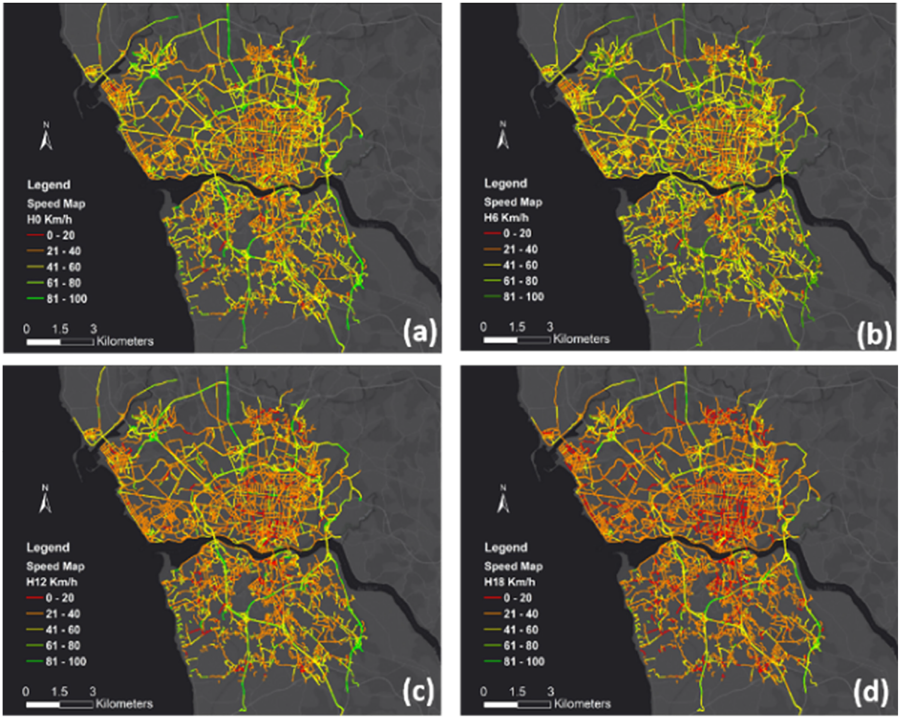
Predicted traffic speed of Porto: (a) traffic speed at midnight, (b) traffic speed at 6 a.m., (c) traffic speed at noon, (d) traffic speed at 6 p.m.

Conclusion

As populations in urban areas increase rapidly, traffic forecasting becomes more and more important. Existing methods rely on historical traffic data, which makes it hard to forecast traffic at city scale. In this research, we proposed a method based on SceneGCN that uses scene features extracted from GSV to predict traffic speeds for each hour of the day. Different scene features are extracted from pretrained Resnet18 models are compared and a GCN model is used to predict traffic speed for each hour of the day. The proposed model has the ability to predict traffic speed at city scale, which can serve as a supplement to traffic flow datasets which are usually collected at limited sites. Our method also illustrated the potential of scene features in traffic flow prediction. Further research can be conducted on the basis of this paper, for example, to improve traffic flow prediction by integrating scene features to existing spatiotemporal models. According to the results, we have two conclusions. First, our proposed model can capture the spatiotemporal characteristics of traffic flow. From the forecasted traffic speed map, we find, as suspected, that areas with more human activities, such as the central city, have lower traffic speeds. Also, as suspected, traffic speed changes during commuting hours, and traffic congestion may occur during these hours. Secondly, scene features extracted from GSV images have the potential to be used to estimate the built environment and urban functions. Traffic speed is influenced by human activities and road conditions, and the good performance of our model indicates that these factors can be reflected in the GSV images.

Our proposed model has some limitations. First, we adopt GCN to capture the spatial characteristics of the traffic network. It requires a high-quality traffic network map and any changes to the network may require retraining the model. Second, the quality of GSV images influences the accuracy of our model significantly. Some highways capture features of surrounding buildings, which may cause errors in streets with similar building scenes. Third, even though GSV images can reflect human activities and road conditions to some degree, other characteristics may influence traffic speed, such as the posted speed limitation and density of population, as well as the availability of public transportation. In the future, we plan to adopt more social-economic factors and urban points of interest (POI) data to our model to improve the forecasting accuracy and improve the temporal resolution of our model.