Sage Journals: Discover world-class research

Abstract

Because of the aging of infrastructure, methods are explored by which the reliability of existing bridges and viaducts can be assessed. In cases in which limited information of the structure is available or its condition is of concern, proof load testing may be used to demonstrate sufficient live load carrying capacity. Proof load tests in the U.S.A. are typically performed using the Manual for Bridge Evaluation (MBE) published by the American Association of State Highway and Transportation Officials (AASHTO). The proof load is expressed by the regular live load model magnified by the target proof load factor. The level of reliability obtained using the target proof load factor is not explicitly stated in the MBE, but is of particular interest. In this article, relevant background documents are investigated to uncover the underlying calculations, assumptions, and input data. Current challenges in proof load testing are described in which the considerations of time dependence, stop criteria, available information, and system-level assessment are highlighted. Subsequently, improvements to the MBE proof load testing background are suggested. An example calculation using traffic data from the Netherlands shows that the HL93 load model and Eurocode LM1 provide a reasonably constant proof load factor with span length for bending and shear. However, the HS20 load model does not scale well with increasing span length. It is found that the magnitude of the target load as specified through the proof load factor is directly related to the desired level of reliability. Although the MBE proof load testing method is practical, several challenges remain.

Keywords

infrastructure structures testing and evaluation of transportation structures bridge assessment load rating load testing

Normally, a structure that has just been completed fulfills functional and safety requirements as specified by the prevailing design standards. However, after years of use, the environment or societal demands may have changed (for instance, larger traffic intensity or more stringent safety requirements). In addition, the structure may have suffered from degradation. To evaluate if the structure fulfils the requirements, an assessment needs to be carried out ( 1 ). Proof load testing is one of the methods available for assessment, competing with desk studies that often make use of finite element models.

Recent advances concern the usage of load test information to update finite element models and structural reliability estimations ( 2 ), and are collected in the Transportation Research Board (TRB) circular Primer on Bridge Load Testing ( 3 ). Proof load testing as a means to assess the structural reliability found its way into the literature in the 1980s ( 4 – 6 ). The probabilistic treatment of proof load testing can result in appropriate target loads depending on the load rating, dead/live load ratios, degradation, bridge age, reference period, and prior service loads ( 7 ). In Europe, proof load factors were developed as part of the large-scale ARCHES (Assessment and Rehabilitation of Central European Highway Structures) project ( 8 ). Recently, efficient strategies for bridge reclassification based on probabilistic decision analysis have gained attention ( 9 – 11 ).

In a proof load test, a relatively large load is applied to a bridge or viaduct to demonstrate sufficient load-carrying capacity. If the structure is able to withstand the large load without showing signs of distress, the test is a success. The load can be applied by using one or more heavy trucks (as is common in the U.S.A.), a loading frame with ballast, or a specialized load testing vehicle (Figure 1). The magnitude of the load to be applied in the proof load test is commonly referred to as the target load. If the target load is chosen to be very large (e.g., multiple times a heavy truck weight), the probability of failure during the test is also large. However, if the bridge can withstand the large load without showing signs of distress, then it has proven to have a high reliability. If a relatively small target load is selected (e.g., a normal truck weight), the probability of failure during the test is small, but it also does not prove that the bridge has high reliability. Therefore, the target load is directly associated with the structural reliability (and safety) of the bridge or viaduct being tested. If the target load could not be reached during the proof load test, because signs of distress were detected, then load posting (load restrictions) may be applied, or the bridge needs to be renovated/replaced. Such decisions depend on the load level reached during the test and the nature of the observed distress.

Figure 1.

The German BELFA load testing vehicle on the Vlijmen-Oost viaduct in the Netherlands. Reprinted with permission from ( 1 ).

In the case in which a proof load test is performed in the U.S.A., the Manual for Bridge Evaluation (MBE) ( 12 ) is used as a guideline. The MBE describes many aspects concerning the inspection and evaluation of existing highway bridges. In this context, proof loading is mentioned as one of the methods in which a load rating may be accomplished. Load rating is the determination of the live load carrying capacity of a structure. The MBE provides guidance on how to use diagnostic and proof load tests for the purpose of load rating. This article focusses on the latter, and in particular the reliability background described in a report dating from 1993 by Lichtenstein ( 13 ), which was also included in the 1998 Manual for Bridge Rating Through Load Testing ( 14 ).

Objective

The objective of this article is to describe the proof load testing method by the American Association of State Highway and Transportation Officials (AASHTO) as provided in the MBE, communicate the background to the target proof load factor (X_p), provide suggestions for improvement, and highlight current challenges in proof load testing—all within the context of structural reliability.

The level of reliability that the MBE proof load testing method provides is of interest in relation to possible application in other countries where different reliability requirements and traffic conditions apply. To aid the knowledge transfer between countries, a significant part of this article is devoted to explaining the MBE proof load testing method and its probabilistic background. The novelty of this research is contained in the improvements suggested to the MBE reliability background and in the identification of the remaining challenges in proof load testing.

Reliability Assessment of Existing Structures

Reliability expresses the probability of success (no failure) within a certain time period, that is, the reference period. In the design of new structures, the reference period is the design life. In the context of annual reliability the reference period is 1 year. Reliability is commonly related to the failure probability via P_f = Φ(−β), where β is the reliability index and Φ(·) indicates the standard normal cumulative distribution function. In the reliability assessment of structures, failure indicates the exceedance of a limit state. Commonly, such a failure comprises loss of capacity or another significant change that leads to an unsafe situation ( 15 ). Reliability assessment of existing structures may be done via various methods, including proof load testing ( 7 ).

The reliability requirements, or targets, for existing structures are commonly lower than the requirements for new structures. For new structures, on top of safety and sociopolitical considerations, additional economy or quality requirements typically govern. In the U.S.A., a reliability index of β = 3.5 with a reference period of 75 years is common for new structures, whereas a reliability index of β = 2.3–2.5 with a reference period of 2–5 years is common for existing structures ( 16 , 17 ). In the U.S.A., a reliability requirement is connected to a failure mode, load combination, and type of uncertainty ( 18 ). Alternatively, a differentiation can be made based on the consequence class (CC) for the structure, as adopted in the Eurocode standards ( 19 ). CC2 is typically associated with bridges in the secondary road network, whilst CC3 applies to structures in the primary (highway) network. The assessment criteria for existing structures in the Netherlands have been determined by a risk-based approach. The minimum allowable annual reliability indices, associated with human safety, are 3.4 for CC2 and 4.0 for CC3 ( 20 ).

Reliability Background of the Manual for Bridge Evaluation Proof Load Testing Method

For a full description of the proof load testing method, the reader is referred to Section 8.8.3 of the MBE ( 12 ). This article is mainly concerned with the calculation of the target load and its relation to structural reliability. Therefore, only the relevant parts of the method are described here.

Rating Factor

The MBE uses a so-called rating factor to indicate to which degree a structure is able to carry live loads. In principle every bridge is thought to have a resistance (or capacity) R, dead load (or self-weight) D, and a live load (or variable load) L. A structure is considered safe if the resistance is equal to, or larger than, the self-weight plus the live load. The rating factor (RF) is derived as follows:

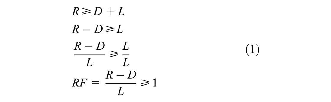
\begin{matrix} R \geq D + L \\ R - D \geq L \\ \frac{R - D}{L} \geq \frac{L}{L} \\ RF = \frac{R - D}{L} \geq 1 \end{matrix}

(1)

In Equation 6A.4.2.1–1 of the MBE additional factors are included, various types of dead load are differentiated, and the dynamic contribution to the live load (dynamic load allowance) is included explicitly.

Target Proof Load

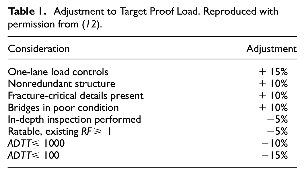
Bridge-specific circumstances may be included via the adjusted proof load factor (X_pA). The proof load factor is increased or decreased by an associated percentage (see Table 1, which is Table 8.8.3.3.1–1 of the MBE). In cases in which multiple considerations apply, the adjustment percentages are summed.

Table 1.

Adjustment to Target Proof Load. Reproduced with permission from ( 12 ).

Consideration	Adjustment
One-lane load controls	+15%
Nonredundant structure	+10%
Fracture-critical details present	+10%
Bridges in poor condition	+10%
In-depth inspection performed	−5%
Ratable, existing RF≥ 1	−5%
ADTT≤ 1000	−10%
ADTT≤ 100	−15%

The value of the adjusted proof load factor is calculated via X_pA = X_p (1 + Σ % / 100). If a one-lane load controls the load effect (i.e., no redistribution of forces between lanes exists), then an increase of 15% is required. The motivation for this adjustment is the 0.85 factor found in comparing two-lane traffic to one-lane traffic loads ( 13 ). The target proof load (L_T) is expressed with respect to the load model and is magnified by an (adjusted) proof load factor, leading to the following expression:

L_{T} = X_{pA} L_{R} (1 + IM)

(2)

where L_R is the comparable unfactored live load because of the rating vehicle for the lanes loaded and IM is the dynamic load allowance (or impact). The background to the target proof load factor (X_p) may be found in the 1998 Manual for Bridge Rating Through Load Testing ( 14 ), which references and attaches a report by Lichtenstein ( 13 ). In Chapter 3 of that technical report, the default value X_p = 1.4 is derived from a probabilistic analysis. The remainder of this section describes the analysis that was performed in the Lichtenstein report ( 13 ) and reproduces the results.

Considered Case

In Lichtenstein ( 13 ), a simply supported bridge with span of l = 60 ft (18.3 m) is considered as a base case. It has two driving lanes and its capacity is unknown. The AASHTO HS20 load effect is calculated by gradually moving the HS20 truck along the beam whilst keeping track of the maximum moment occurring at each location. The HS20 truck is defined by a front axle loaded with 8 kip (35.6 kN), followed at 14 ft (4.27 m) by an axle loaded with 32 kip (142.3 kN) and then by another axle of 32 kip. The distance between the heavily loaded axles is 14–30 ft (4.27–9.14 m), whichever produces the largest load effect—in this case it is 14 ft. The calculated moment envelope is plotted in Figure 2, which indicates a maximum of 807 kip·ft (1094 kNm) around the midspan.

Figure 2.

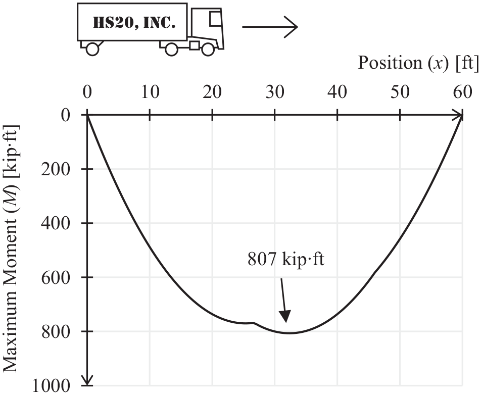
Moment envelope of a 60 ft (18.3 m) simply supported beam subjected to the HS20 load. Conversion factors: 1 ft = 0.305 m, 1 kip·ft = 1.35 kNm.

Limit State Function

The limit state function adopted in the Lichtenstein report ( 13 ) for the probabilistic calculation is as follows:

Z = R - (D + L + I)

(3)

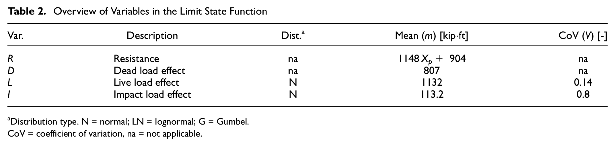
where R is the resistance of the structure, D is the dead load (permanent load), L is the live load, and I is the impact load (dynamic load effect).

In the case in which Z < 0, structural failure occurs. The resistance and dead load are regarded as deterministic values in the calculation. It is assumed that their values are known after the proof load test. The value of the dead load effect is taken to be equal to the AASHTO HS20 live load effect, that is, D = L_A = 807 kip·ft per lane. The effect of different dead load contributions in relation to the live load is studied by Lichtenstein ( 13 ) as well. The live load (L) and impact load (I) are modeled as random variables.

Traffic Load

The mean value of the 75-year maximum traffic load is equal to 1.79 times the HS20 load effect (L_A) as determined by extrapolation of a traffic survey ( 21 ). For a reference period of two years, it is 1.65 times the HS20 load effect. The latter reference period is deemed to be appropriate in the context of proof load testing because it is based on an inspection interval of two years.

If two lanes are considered, a reduction factor of 0.85 applies because of expected redistribution of the load between lanes. The live load has a coefficient of variation of 0.18. This value is thought to cover both the uncertainty in the occurrence of heavy truck loads and the analysis. If only the truck load uncertainty is considered, a reduced value of 0.14 applies. The dynamic load allowance is different than that defined by the coefficient of AASHTO. Its mean value is estimated to be about 0.1 of the live load, with a coefficient of variation of 0.8. The mean value of the live load for a return period of 2 years is thus calculated as follows:

m_{L} = 0.85 \cdot 1.65 \cdot 807 = 1132 kip \cdot ft (1535 kNm)

Only the uncertainty in the occurrence of heavy truck loads is deemed to apply, and therefore the coefficient of variation V_L = 0.14 is used. The mean value of the impact load is calculated as follows:

m_{I} = 0.1 \cdot 1132 = 113.2 kip \cdot ft (153.5 kNm)

with coefficient of variation V_I = 0.8.

Resistance

If the proof load test was successful, the resistance of the structure is at least equal to the sum of the target proof load (L_T) and the dead load. In the probabilistic analysis the mean resistance of the structure is calculated as follows:

R = 1.12 (L_{T} + D) = 1.12 [X_{p} L_{A} (1 + C_{I, A}) + D]

(4)

where the factor 1.12 accounts for higher mean strengths in respect to the nominal (or “design”) strengths used in regular code calculations. The value of the AASHTO impact coefficient for 60 ft (18.2 m) is C_I,A = 50/(60 + 125) = 0.27. The resistance for this case is calculated as follows:

\begin{matrix} R = 1.12 [X_{p} \cdot 807 (1 + 0.27) + 807] \\ = 1148 X_{p} + 904 kip \cdot ft \end{matrix}

All information required to perform the probabilistic analysis has now been described. Table 2 provides an overview of the parameters used in the limit state function.

Table 2.

Overview of Variables in the Limit State Function

Var.	Description	Dist.^a	Mean (m) [kip·ft]	CoV (V) [-]
R	Resistance	na	1148 X_p + 904	na
D	Dead load effect	na	807	na
L	Live load effect	N	1132	0.14
I	Impact load effect	N	113.2	0.8

Distribution type. N = normal; LN = lognormal; G = Gumbel.

CoV = coefficient of variation, na = not applicable.

Results

Since all distributions are assumed to be normal, the calculation method in Lichtenstein ( 13 ) simply consists of dividing the mean value of the limit state function Z by its standard deviation. Making use of the first-order reliability method (FORM) ( 22 ) is also possible. In this case, the FORM converges to the exact solution in one iteration. The reliability index (β) that results from the probabilistic calculation for various values of X_p is provided in Table 3. The values in the column Recalculated have been obtained by the author and are in correspondence with the original numbers.

Table 3.

Calculated Reliability with Increasing Proof Load Factor

Proof load factor (X_p) [-]	Reliability index for 2 years (β) [-]
Proof load factor (X_p) [-]	Lichtenstein	Recalculated
1.2	1.26	1.26
1.3	1.89	1.89
1.4	2.57	2.52
1.5	3.15	3.15
1.6	3.78	3.77

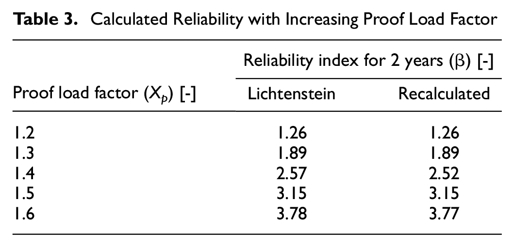
The value X_p = 1.4 was selected because a reliability index of β = 2.3 was found to be in line with the operating level according to the AASHTO Load and Resistance Factor Design (LRFD) studies ( 16 ). The reliability index is lower than that used for the inventory and design level. The lower value is justified, since it reflects past rating practices at the operating level. In relation to varying span lengths, two additional calculations are performed by Lichtenstein ( 13 ). It is concluded that the factor X_p = 1.4 provides adequate safety for other spans as well.

Suggested Improvements to the Manual for Bridge Evaluation Proof Load Testing Background

In this section various improvements are suggested to be incorporated into the background of the MBE proof load testing method. It does, however, not result in a ready-to-be-adopted new format. Instead, the most important facets are highlighted and improvements are suggested.

Probabilistic Model

In the Lichtenstein report ( 13 ), the dead load is treated as a deterministic value equal to the live load. The value of the dead load (effect) is not exactly known, as it is generally not possible to measure its value. However, because the structure can carry the dead load, it does not matter if it is lower or higher than expected. When including the dead load as a random variable, it can also be eliminated from the limit state function, as shown in Equation 5.

An additional factor of 1.12 is used in Equation 4 to convert from nominal to mean strength. Such a factor is appropriate when R is a design or nominal strength. However, here R is a random variable. After a successful proof load test, it is known that the resistance must be equal to or larger than the load effect following from the self-weight and the target load (R ≥ D + L_T). Assigning the resistance with a value that is 12% higher than that obtained from the test is speculative.

With the suggested alterations, the limit state function may be rewritten such that only the live load and the dynamic amplification remain as random variables. In essence, the probability of failure of the structural part or cross-section is directly reformulated into the probability that a future live load effect (including dynamic amplification) exceeds the load effect produced during the proof load test:

\begin{matrix} Z = R - (D + L + I) \\ = (D + L_{T}) - (D + L + I) \\ = L_{T} - (L + I) \end{matrix}

Here, L_T is the target proof load effect (deterministic value), L is the traffic live load effect (random variable), and I is the dynamic contribution (random variable).

The dynamic load effect (impact) should be included in the target load (L_T) as part of the load model via the regular design procedure. Since comparable extreme values for the traffic load are considered, the design procedure to account for the dynamic loads is suitable here as well. Therefore, the impact (I) may be removed from the limit state function. In this way, the probabilistic analysis can be performed using recorded traffic loads without, or with minimal, dynamic contribution (e.g., weight-in-motion [WIM] data).

Missing in the limit state function of Equation 5 are model uncertainties. Our understanding of the translation from applied loads, in a test or from actual traffic, to the load effect is limited. The degree of uncertainty depends on the level of sophistication incorporated in the mechanical model. Additional uncertainty stems from the statistical modeling of the load effect—that is, the assumed distribution functions. The variability of the traffic load may be split into time-invariant (C_0L) and time-variant parts (L) ( 23 ). By including model uncertainties, splitting the live load variability, and removing the dynamic contribution, the limit state function becomes as follows:

Z = θ_{LT} L_{T} - θ_{L} C_{0 L} L

(6)

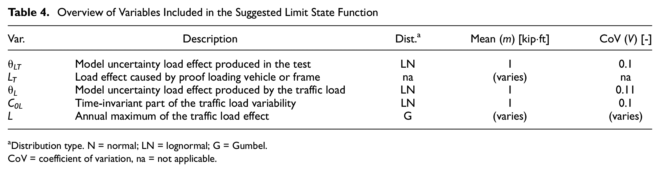
An overview and description of the parameters in the suggested limit state function is provided in Table 4. The statistical properties of the random variables are based on general recommendations for probabilistic modeling ( 23 , 24 ). The coefficient of variation of the model uncertainty concerning the load effect produced in the proof load test (θ_LT) is based on the value of the model uncertainty related to the traffic load. Because the conditions are more controlled during a test, a lower value may seem more appropriate. However, when viewed as a resistance parameter, it should also cover the uncertainty associated with selecting the most critical locations to test. This issue is alleviated when using a moving vehicle to perform the test, but also here some uncertainty remains related to the transverse location and axle configuration.

Table 4.

Overview of Variables Included in the Suggested Limit State Function

Var.	Description	Dist.^a	Mean (m) [kip·ft]	CoV (V) [-]
θ_LT	Model uncertainty load effect produced in the test	LN	1	0.1
L_T	Load effect caused by proof loading vehicle or frame	na	(varies)	na
θ_L	Model uncertainty load effect produced by the traffic load	LN	1	0.11
C_0L	Time-invariant part of the traffic load variability	LN	1	0.1
L	Annual maximum of the traffic load effect	G	(varies)	(varies)

Distribution type. N = normal; LN = lognormal; G = Gumbel.

CoV = coefficient of variation, na = not applicable.

The mean value of the model uncertainty relating to the traffic load effect (θ_L) can be altered to introduce a certain bias. In this way, a traffic load model derived on the basis of roads with great intensity may be corrected with a factor lower than 1 to reflect the general case. On the other hand, the trend of continuously increasing traffic loads would increase the mean value. The latter depends largely on the time period that is considered. The trend will also depend on the span length (or influence length) because of longer trucks and smaller inter-vehicle distances, for example, truck platooning ( 25 ). This affects large spans more than short spans.

Traffic Load

In the Lichtenstein report ( 13 ), the statistical description of the live load and impact (dynamic) load is based on the study by Nowak from 1993 ( 21 ). It is recommended to use more recent data, preferably obtained from the measurement of axle loads at multiple locations and for a longer period of time (e.g., one year or more). WIM data is well-suited to obtain an accurate statistical representation of the traffic load effect.

In the Netherlands, WIM recording stations are positioned at several traffic-intense highway locations. Using WIM data from 2015 in the Netherlands, traffic simulations have been performed to obtain the maximum bending moment at the midspan and the maximum shear force near the supports of a simply supported span. Over a period of one year, various block maxima may be determined: hourly, daily, weekly, and so on. Considering the difference in traffic on weekdays and at the weekend, a week represents an appropriate cycle, leading to 52 data points. Subsequently, the Gumbel extreme value distribution is fitted to the data using the maximum likelihood estimation (MLE) method. A threshold value is chosen (probability of exceedance S = 0.25) to capture, on the log-scale, the linearly descending right-hand tail of the distribution. Figure 3 shows the fitted distribution to the data points of the maximum bending moment of Dutch highway A27L lane 1—the rightmost lane mostly occupied by trucks.

Figure 3.

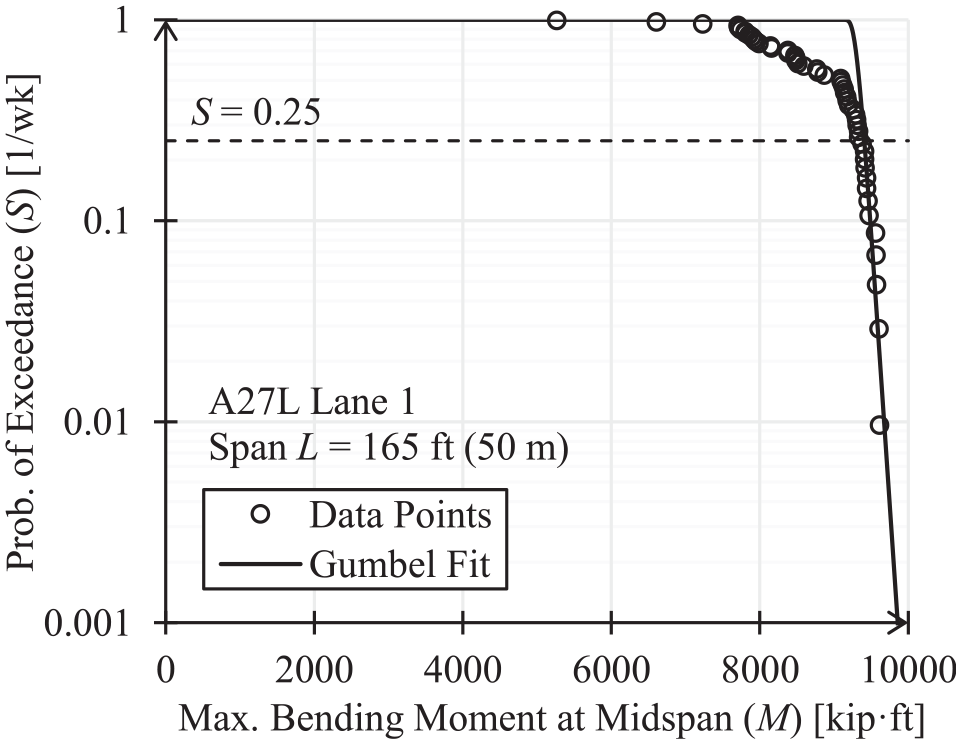
Gumbel fit of the load effect data points for the maximum bending moment at the midspan of a simply supported span. Conversion factors: 1 ft = 0.305 m, 1 kip·ft = 1.35 kNm.

The traffic load model uncertainty incorporated in the probabilistic model should reflect the quality of the data and its modeling. Ideally, data collected over a long period of time is used for distribution fitting. However, traffic data from many years ago may not be representative for the traffic today. Over longer periods of time, trends in the data may cause a distorted view if all data points are processed as if they would have originated from the same stationary process.

Because the weekly maxima are sufficiently uncorrelated, the Gumbel distribution may be converted to annual maxima by shifting the location parameter (μ) via μ_a = μ_w + β_G ln(52), where β_G is the scale parameter and 52 is the number of weeks in a year. The mean and coefficient of variation of the distribution are obtained as m = μ + β_Gγ and V = s / m = (β_G π / √6) / m, where γ ≈ 0.5772 is the Euler–Mascheroni constant ( 26 ). Distributions have been fitted for various WIM datasets and span lengths, as displayed in Figure 4. The analyzed roads show a comparable trend in the mean and coefficient of variation with span length. In a reliability analysis, the average of the four different roads is used (plus model uncertainty θ_L; see Table 4).

Figure 4.

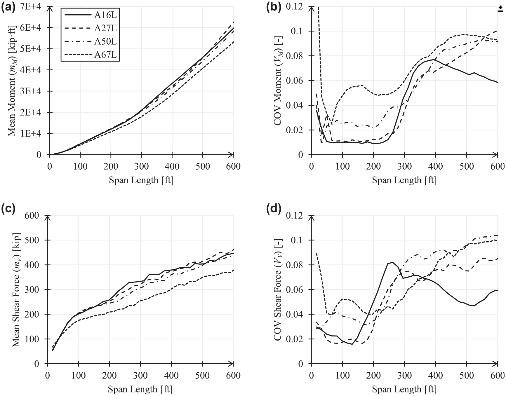
Parameters of the fitted Gumbel distribution for the annual maximum load effect: (a) mean of the bending moment, (b) coefficient of variation (COV) of the bending moment, (c) mean of shear force, and (d) coefficient of variation of shear force. Conversion factors: 1 ft = 0.305 m, 1 kip·ft = 1.35 kNm, 1 kip = 4.45 kN.

Influence of Span Length

The configuration of a bridge that is subjected to a proof load test is often different than the simply supported span for which the load effect was calculated and the reliability analysis was performed. To overcome this limitation, the target proof load is related to a load model via the proof load factor; see Equation 2. In the Lichtenstein report ( 13 ) the HS20 load model is used, but today the HL93 load model ( 16 ) describes the traffic better. In addition to an HS20 truck or a (military) load tandem, the latter also includes a lane load (distributed load) that represents the other traffic present on the bridge. The HL93 load model is comparable to the Eurocode LM1 specification but has significantly lower loads. In Nowak et al. ( 27 ) it is found that the Eurocode LM1 load effects are about a factor two higher than those calculated using AASHTO HL93, owing to the higher unfactored loads in the traffic model. After applying (partial) factors, the design load effect varies from country to country.

To study the relation between the span length and the target proof load factor, an example calculation is made with the improved probabilistic model and traffic data from the Netherlands. Per the span length, two probabilistic analyses are performed: one considering the bending moment at the midspan and one considering the shear force near the supports. CC2 and CC3 of EN 1990 ( 19 ) are considered with target annual reliability indices of 3.4 and 4.0, respectively. The distributed load of the Eurocode LM1 and the AASHTO HL93 load models are applied over a lane width of 3 m. The proof load factors following from the reliability analyses are displayed in Figure 5.

Figure 5.

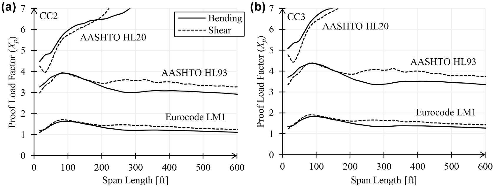
Relation between the span length and target proof load factor considering unfactored load models in the bending and shear: (a) consequence class (CC) 2 with annual reliability requirement β = 3.4 and (b) consequence class 3 with annual reliability requirement β = 4.0. Conversion factor: 1 ft = 0.305 m. AASHTO = American Association of State Highway and Transportation Officials.

It is observed that the target proof load factor is considerably larger when using the AASHTO HS20 and HL93 load models in comparison to Eurocode LM1. This follows from the relatively high unfactored load effect following from LM1. A quick comparison of the axle loads signifies the difference: 67.4 kip (300 kN) for LM1 versus 32 kip (145 kN) for HS20 and HL93, respectively. The traffic load from the Netherlands is relatively high compared to other countries ( 28 ) and meshes with the high loads of Eurocode LM1, leading to moderate values of the proof load factor (X_p). Because of the large discrepancy between unfactored load models, it is recommended to cautiously evaluate traffic models and statistical descriptions for application within the U.S.A.

Another observation is the continuously increasing proof load factor with span length when the HS20 load model is used. This is because the load model only includes a single truck, whereas in reality many vehicles may be present on the bridge. The issue is overcome by the HL93 load model, which also includes a distributed lane load. For both the Eurocode LM1 and the HL93 load models, an almost constant factor is obtained over various spans. Only around 100 ft (30 m) is a relatively large factor is required. This may be explained by the occurrence of long and heavy vehicles (an oversize load for which usually an exemption must be requested) that are not accurately represented by the load model.

Remaining Challenges in Proof Load Testing

In the more general context of proof load testing, several current challenges are highlighted in relation to structural reliability. Because the practice of proof load testing has been established in the past, where assessments had a predominantly deterministic character, various probabilistic aspects deserve extra attention. The aspects highlighted below could provide further advancement of the reliability background (and suggestions for improvement) presented in the previous sections.

Time Dependence

The structural reliability of a bridge or viaduct that is subject to time-variant loads (such as traffic loads), or other time-dependent processes, is not constant in time ( 29 ). It is intuitive to understand that the reliability of a bridge or viaduct that suffers from corrosion, or any other form of degradation, will slowly decrease with time. Less intuitive is the increase of reliability with time as the bridge continuously sustains a high traffic load, and thus displays proven strength with time. Both of these effects result in a variable conditional failure probability, often in the form of a bathtub curve ( 30 ). Conditional indicates the condition in which no failure has occurred in the past. By considering a sufficiently small period of time, the evolution of structural reliability may be followed. To this end, the annual reliability is considered in time-dependent probabilistic calculations ( 31 ). When a proof load test is performed, the failure probability is high because of the large load that is applied. Afterwards, in the case of a successful test, the structural reliability is higher ( 32 ). The bathtub curve may be extended to include a proof load test, as displayed in Figure 6.

Figure 6.

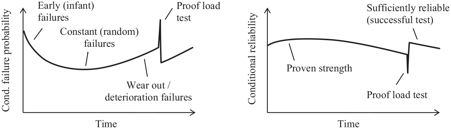
Evolution of conditional failure probability and (annual) reliability with time.

When a proof load test is successful, a sufficient degree of structural reliability is demonstrated at that moment. However, because of the time-dependent effects (such as deterioration and traffic load trends) the reliability may not be sufficient in the future. Substantiated statements about the development of future reliability require probabilistic analyses in which time-dependent effects are explicitly considered ( 33 ). An appropriate increase of the target load (e.g., via the factor X_pA) may be quantified, depending on the bridge-specific circumstances. In this way, the expected time-dependent effects and their uncertainty can be compensated by a higher target load.

Stop Criteria

During a proof load test the load is gradually increased until the target load is reached. In this process, the structure may show signs of distress before the full target load is applied. Therefore, criteria for stopping the proof test are required. The use of sensors during the test provides extra information about the structural response. The stop criteria are typically related to the structural response (not directly the measurements). The sensor readings are interpreted with respect to stop criteria. If a stop criterion is exceeded in the proof load test, irreversible damage may occur. Depending on the damage and failure mechanism, different stop criteria apply ( 34 , 35 ).

Many bridges are constructed using reinforced concrete. Generic stop criteria are difficult to apply in practice for reinforced concrete structures where there may be existing cracks caused by material degradation ( 3 ). In addition, a distinction between linear and non-linear behavior is not useful as a stop criterion because even moderate loads can cause the exceedance of the concrete tensile strength. In some cases small cracks are acceptable, while in other cases they are not.

In the definition and application of stop criteria, little attention is paid to the link with structural reliability. By considering the reliability during the test, the risk of collapse can be mitigated and additional guidance provided for the selection and placement of sensors ( 36 ).

Information About the Structure and Its Context

The knowledge level (available information in drawings, calculations, material tests, etc.) may vary significantly between structures ( 8 ). For older structures it is common that documentation is missing and only basic information (year of construction, geometry, etc.) remains. Valuable information may also relate to the context of the structure. For example, a bridge may be part of the highway network or part of a larger group of infrastructure all designed to the same specifications.

Many information sources can be included to estimate the capacity of a structure. In addition, extra material tests may be performed to obtain a better estimate of the important parameters in the structural model. Ultimately, a balance must be sought between acquiring information about the structural performance and with respect to the proof load test as the main source of information ( 9 ). Through the application of Bayes’ theorem, various sources of information (evidence) can be included to improve the estimate of the resistance. For this purpose, the uncertainty of the resistance is split into the objective (natural) and subjective (model) parts. In this way, the model uncertainty may be systematically updated in the Bayesian approach ( 5 ).

System-level Assessment

A bridge or viaduct consists of several components, such as the deck, girders, supports, and so forth. In addition, cross-sections and connections can also be regarded as components. In the calculation of the structural reliability of the entire structure, all components matter. In regular design approaches, the reliability is verified at the structural component or element level. Under the assumption of sufficient parallel performance (redundancy), correlation between the components or overstrength, the system reliability is approximately equal to the reliability at element level. However, this single component methodology may actually lead to both under- and overconservative designs ( 37 ). Explicitly considering the system behavior in the probabilistic assessment leads to more accurate estimates of structural reliability.

Checking only a single cross-section (e.g., the bending moment capacity at the midspan) in a proof load test is not always sufficient to verify the reliability of the bridge as a whole. In this regard, the MBE states that “loads must also be moved to different positions to properly check all load path components.” In practice this is accomplished by using various heavy vehicles and driving paths.

Because of practical limitations or economic reasons, not all components may be verified explicitly in a proof load test. Bayesian analysis can be used to update the reliability of the system with information about a limited number of components ( 38 ). In this way, uncertainty may be compensated through application of a higher target load.

Discussion

Suggested Improvements

The suggested probabilistic model includes model uncertainties for both the actual live load (θ_L) and the live load produced in a proof load test (θ_LT). Their statistical description has been estimated and requires further refinement. In particular, the uncertainty associated with the proof load test will need to cover different aspects depending on the application: how the load is applied, how many positions and lanes are tested, whether the bending or shear are critical, and so forth. In addition, it is likely that the model uncertainties (θ_LT and θ_L) are correlated because the same mathematical principles/models are used to calculate both load effects. Because there are several remaining challenges, the probabilistic model and the results presented in this article should be viewed as indicative.

The traffic load analysis was performed using highway measurements obtained in the Netherlands; therefore, the resulting distributions have limited applicability. By using the method followed in this article, applicable distributions can be derived for different countries. For completeness, also other configurations besides the single span case need to be considered ( 8 ).

In the MBE an adjustment to the target live load of +15% is suggested in cases in which a one-lane load controls the load effect. This is a measure to counteract the more favorable two-lane traffic load description used by Lichtenstein ( 13 ). An important assumption in the two-lane situation is that the bridge is able to redistribute the traffic load between its lanes. This is not always the case. In today’s computer-aided design process, all lanes and their corresponding loads are included in the model. The load effect for additional lanes follows from the load model, just as in the design calculation. (The rationale is the same for excluding the dynamic effect in the probabilistic calculation; it is assumed that the established calculation rules account for these particularities correctly.) The use of a multiple presence factor (MPF) calibrated on the basis of WIM data is recommended ( 39 ). With the one-lane situation as the default, a probabilistic assessment of the first lane (as performed in this article) will correspond to MPF = 1.0.

Remaining Challenges

Proof load testing is a valuable tool to demonstrate sufficient load-carrying capacity. However, the derivation of load factors and rules to carry out a test that results in the desired reliability remains challenging.

The time dependence of the structural reliability can be incorporated into a probabilistic analysis directly to deliver the point in time where the annual reliability is not sufficient any longer. An example of such a calculation is provided by De Vries et al. ( 33 , 40 ). If such analyses are performed for several typical cases, the required increase of the target load can be determined.

A future framework for proof load testing should be flexible with respect to which information is utilized. In some cases, bridge documentation, material data, traffic data, or even proof load testing data on similar bridges may be available. It would not be economical to ignore evidence of good structural performance. Additional rules may be established on the basis of Bayesian inference to utilize knowledge about the structure and its context (traffic loads, environment, geographical location, etc.) ( 33 ).

By thinking about the bridge as a system of components, the question is how many components are tested in a proof load test. This may also depend on the type of bridge or failure mechanism being considered. In a (successful) proof load test, one can only observe that the system (i.e., the entire structure) carries the load. However, the load may not follow the expected load path and/or redistribution of forces can take place. For this reason, the proof load test result does not necessarily tell us something about the performance of a component.

Conclusion

The magnitude of the target load is directly related to the desired level of reliability. In the MBE ( 12 ), the target load is obtained through application of the live load model multiplied by a factor for proof load testing that can also include bridge-specific adjustments (X_pA). In this way, the target proof load can be easily calculated for any bridge or viaduct under consideration. The background report by Lichtenstein ( 13 ) was studied to uncover the underlying probabilistic model. The calculations resulting in the basic value of X_p = 1.4 as used in the MBE have been reproduced with success.

Although a method based on the probabilistic analysis of the live load alone (such as the MBE method) is practical, several challenges remain: the influence of time-dependent effects, reliability of stop criteria, usage of information about the structure, and the importance of system-level assessment. Only a part of the challenges can be overcome by adjustments to the target load or factor. Verifying the reliability of an existing bridge or viaduct through proof load testing is markedly different from the design process.

The main idea behind the MBE method (i.e., the resistance is at least equal to the self-weight and the applied live load in the test) remains valuable and therefore suggestions for improvement have been provided. In summary, the improvements entail including model uncertainties in the probabilistic model, updating the traffic load description, and adopting the appropriate live load model. Dutch roads with high traffic intensity display a comparable trend in the statistical description of the load effect with span length. With a probabilistic analysis it was shown that live load models HL93 and Eurocode LM1 can provide reasonably constant proof of load factors over a large range of span lengths, for both bending and shear.

Footnotes

Appendix

Acknowledgements

The authors wish to express their gratitude and sincere appreciation for the fruitful discussions with Sonja A.A.M. Fennis of Rijkswaterstaat and Max A.N. Hendriks from Delft University of Technology, which have been of great help.

Author Contributions

The authors confirm contribution to the paper as follows: study conception and design: E. Lantsoght, R. Steenbergen, R. de Vries; data collection: R. de Vries; analysis and interpretation of results: R. de Vries, E. Lantsoght, R. Steenbergen, M. Naaktgeboren; draft manuscript preparation: R. de Vries, E. Lantsoght, R. Steenbergen, M. Naaktgeboren. All authors reviewed the results and approved the final version of the manuscript.

Declaration of Conflicting Interests

The author(s) declared no potential conflicts of interest with respect to the research, authorship, and/or publication of this article.

Funding

The author(s) disclosed receipt of the following financial support for the research, authorship, and/or publication of this article: This work was supported by the Dutch Ministry of Infrastructure and Water Management (Rijkswaterstaat).

ORCID iD

Marius Naaktgeboren

References

Lantsoght

E. O. L.

van der Veen

de Boer

Hordijk

D. A.

State-of-the-Art on Load Testing of Concrete Bridges. Engineering Structures, Vol. 150, 2017, pp. 231–241.

Alampalli

Frangopol

D. M.

Grimson

Halling

M. W.

Kosnik

D. E.

Lantsoght

E. O. L.

Yang

D. Y.

Zhou

Bridge Load Testing: State-of-the-Practice. Journal of Bridge Engineering, Vol. 26, No. 3, 2021, p. 03120002.

Alampalli

Frangopol

D. M.

Grimson

Kosnik

Halling

Lantsoght

E. O. L.

Weidner

J. S.

Yang

D. Y.

Zhou

Y. E.

Primer on Bridge Load Testing, TRB Circular E-C257. Transportation Research Board, Washington, D.C., 2019.

Grigoriu

Hall

W. B.

Probabilistic Models for Proof Load Testing. Journal of Structural Engineering, Vol. 110, No. 2, 1984, pp. 260–274.

Lin

T. S.

Nowak

A. S.

Proof Loading and Structural Reliability. Reliability Engineering, Vol. 8, 1984, pp. 85–100.

Rackwitz

Schrupp

Quality Control, Proof Testing and Structural Reliability. Structural Safety, Vol. 2, 1985, pp. 239–244.

Faber

M. H.

Val

D. V.

Stewart

M. G.

Proof Load Testing for Bridge Assessment and Upgrading. Engineering Structures, Vol. 22, 2000, pp. 1677–1689.

Casas

J. R.

Gómez

J. D.

Load Rating of Highway Bridges by Proof-Loading. KSCE Journal of Civil Engineering, Vol. 17, No. 3, 2013, pp. 556–567.

Medha

Schmidt

J. W.

Sørensen

J. D.

Thöns

A Decision Theoretic Approach Towards Planning of Proof Load Tests. 13th International Conference on Applications of Statistics and Probability in Civil Engineering (ICASP), Seoul, South Korea, 2019.

10.

Schmidt

J. W.

Thöns

Kapoor

Christensen

C. O.

Engelund

Sørensen

J. D.

Challenges Related to Probabilistic Decision Analysis for Bridge Testing and Reclassification. Frontiers in Built Environment, Vol. 6, 2020, p. 14.

11.

Zhang

W. H.

D. G.

Qin

Thöns

Faber

M. H.

Value of Information Analysis in Civil and Infrastructure Engineering: A Review. Journal of Infrastructure Preservation and Resilience, Vol. 2, 2021, p. 16.

12.

American Association of State Highway Transportation Officials. The Manual for Bridge Evaluation, Standard, 3rd ed. AASHTO, Washington, D.C., 2018.

13.

Lichtenstein

A. G.

Bridge Rating Through Nondestructive Load Testing. Technical Report, NCHRP Project 12-28(13)A, TRB, National Research Council, Washington, D.C., 1993.

14.

NCHRP. Manual for Bridge Rating Through Load Testing, Research Results Digest, No. 234. Transportation Research Board (TRB), Washington, D.C., 1998.

15.

Madsen

H. O.

Krenk

Lind

N. C.

Methods of Structural Safety. Prentice Hall, Englewood Cliffs, New Jersey, 1986, p. 403.

16.

American Association of State Highway Transportation Officials. LRFD Bridge Design Specifications, Standard, 9th ed. AASHTO, Washington, D.C., 2020.

17.

NCHRP. Load Capacity Evaluation of Existing Bridges. Report 301, Project 12-28(1), TRB, National Research Council, Washington, D.C., 1987.

18.

Bhattacharya

Chajes

Hastings

Reliability-Based Load and Resistance Factor Rating Using in-Service Data. Journal of Bridge Engineering, Vol. 10, No. 5, 2005, pp. 530–543.

19.

CEN. Eurocode 0: Basis of Structural Design. Standard, EN 1990+A1+A1/C2:2019, European Committee for Standardization, Brussels, Belgium, 2019.

20.

Steenbergen

R. D. J. M.

Vrouwenvelder

A. C.W. M.

Safety Philosophy for Existing Structures and Partial Factors for Traffic Loads on Bridges. Heron, Vol. 55, No. 2, 2010, pp. 123–139.

21.

Nowak

A. S.

Live Load Model for Highway Bridges. Structural Safety, Vol. 13, No. 1–2, 1993, pp. 53–66.

22.

Hasofer

A. M.

Lind

N. C.

Exact and Invariant Second-Moment Code Format. Journal of the Engineering Mechanics Division, Vol. 100, No. 1, 1974, pp. 111–121.

23.

fib. Partial Factor Methods for Existing Concrete Structures. Bulletin 80, Recommendation, Task Group 3.1, Fédération internationale du béton, 2016.

24.

JCSS. Probabilistic Model Code. 2015. https://www.jcss-lc.org/jcss-probabilistic-model-code/

25.

Thulaseedharan

Yarnold

M. T.

Prioritization of Texas Prestressed Concrete Bridges for Future Truck Platoon Loading. Bridge Structures, Vol. 16, No. 4, 2020, pp. 155–167.

26.

Gumbel

E. J.

Statistical Theory of Extreme Values and Some Practical Applications. Applied Mathematics Series, National Bureau of Standards, Washington, D.C., Vol. 33, 1954.

27.

Nowak

A. S.

Lutomirska

Sheikh Ibrahim

F. I.

The Development of Live Load for Long Span Bridges. Bridge Structures, Vol. 6, No. 1, 2010, pp. 73–79.

28.

O’Brien

E. J.

O’Connor

A. J.

Arrigan

J. E.

Procedures for Calibrating Eurocode Traffic Load Model 1 for National Conditions. Proc., 6th International Conference on Bridge Maintenance, Safety and Management (IABMAS 2012), Stresa, Italy, 2012, pp. 2597–2603.

29.

Enright

M. P.

Frangopol

D. M.

Probabilistic Analysis of Resistance Degradation of Reinforced Concrete Bridge Beams Under Corrosion. Engineering Structures, Vol. 20, No. 11, 1998, pp. 960–971.

30.

Smith

D. J.

Understanding Terms and Jargon. In Reliability, Maintainability and Risk, 7th ed., (D. J. Smith, Butterworth-Heinemann, eds.), Oxford, UK, 2005, pp. 11–23.

31.

Melhem

M. M.

Caprani

C. C.

Stewart

M. G.

Zhang

Bridge Assessment Beyond the AS 5100 Deterministic Methodology. Research Report AP-R617-20, Austroads, 2020.

32.

Spaethe

Die Beeinflussung Der Sicherheit Eines Tragwerks Durch Probebelastung. Bauingenieur, Vol. 69, 1994, pp. 459–468.

33.

De Vries

Lantsoght

E. O. L.

Steenbergen

R. D. J. M.

Fennis

S. A. A. M.

Reliability Assessment of Existing Reinforced Concrete Bridges and Viaducts Through Proof Load Testing. Proc., IABMAS Conference, Barcelona, Spain, 2022.

34.

DAfStb. DAfStb-Richtlinie: Belastungsversuche an Betonbauwerken. Guideline, Deutscher Ausschuss für Stahlbeton, Berlin, Germany, 2020.

35.

Zarate Garnica

G. I.

Lantsoght

E. O. L.

Stop Criteria for Proof Load Testing of Reinforced Concrete Structures. Proc., 2021 Session of the 13th fib International PhD Symposium in Civil Engineering, Paris, France, 2021, pp. 195–202.

36.

Zarate Garnica

G. I.

Lantsoght

E. O. L.

Yang

Monitoring Structural Responses During Load Testing of Reinforced Concrete Bridges: A Review. Structure and Infrastructure Engineering, Vol. 18, No. 10–11, 2022, pp. 1558–1580.

37.

Hendawi

Frangopol

D. M.

System Reliability and Redundancy in Structural Design and Evaluation. Structural Safety, Vol. 16, 1994, pp. 47–71.

38.

Schneider

Time-Variant Reliability of Deteriorating Structural Systems Conditional on Inspection and Monitoring Data. PhD thesis, Technical University of Munich, Bundesanstalt für Materialforschung und -prüfung (BAM), Munich, 2020.

39.

Liu

Bowman

Multiple Presence Factor for Truck Load on Highway Bridges. Journal of Bridge Engineering, Vol. 18, No. 3, 2013, pp. 240–249.

40.

De Vries

Lantsoght

E. O. L.

Steenbergen

R. D. J. M.

Case Study Proof Loading in an Annual Reliability Framework. Stevin Report 25.5-21-02, Delft University of Technology, Delft, The Netherlands, 2021.

Proof Load Testing Method by the American Association of State Highway and Transportation Officials and Suggestions for Improvement

Abstract

Keywords

Objective

Reliability Assessment of Existing Structures

Reliability Background of the Manual for Bridge Evaluation Proof Load Testing Method

Rating Factor

Target Proof Load

Considered Case

Limit State Function

Traffic Load

Resistance

Results

Suggested Improvements to the Manual for Bridge Evaluation Proof Load Testing Background

Probabilistic Model

Traffic Load

Influence of Span Length

Remaining Challenges in Proof Load Testing

Time Dependence

Stop Criteria

Information About the Structure and Its Context

System-level Assessment

Discussion

Suggested Improvements

Remaining Challenges

Conclusion

Footnotes

Appendix

Acknowledgements

Author Contributions

Declaration of Conflicting Interests

Funding

ORCID iD

References