Sage Journals: Discover world-class research

Abstract

Reliability has been incorporated in pavement design tools to account for input variability influence on predicted performance. As they are not based on a probabilistic method of uncertainty propagation, the reliability analysis methodologies that are currently implemented in pavement performance tools lack rigor and robustness. This paper investigates the potential of three reliability analysis methodologies for pavement application: the Pavement ME reliability analysis methodology, Monte Carlo simulation (MCS), and the first-order reliability method (FORM). The MCS and FORM involve a response surface method for the generation of a second-order surrogate model. The investigation was performed using inputs and performance data from accelerated pavement testing structures. Inputs that were identified as significant were characterized as random variables and their associated variability was established using measured structural and material properties. Pavement performance with respect to rutting was predicted using the ERAPave performance prediction tool, while MCS was used to generate the actual variability of the distress. The reliability analysis results have shown that a comprehensive reliability analysis methodology is required that effectively captures input variabilities and the error associated with surrogate models.

Keywords

variability MCS pavement ME RSM reliability ERAPave PP FORM

The pavement design process is probabilistic, as it involves uncertainties that originate from different sources ( 1 ). The impact of these uncertainties on predicted performance should be addressed and mitigated as this would allow maintenance and rehabilitation interventions that are timely and cost effective. This will consequently lower the total life cycle cost estimate of highway projects ( 2 ). Many pavement design procedures have incorporated reliability into the design process to account for input variability influence on predicted performance. Reliability is computed in these design procedures by utilizing different reliability analysis methodologies and using variabilities that are characterized and quantified on the basis of various assumptions, making it challenging to perform a direct comparison across pavement design procedures ( 3 – 5 ). A reliability analysis methodology that is comprehensive in nature and that characterizes input variability through statistically sound methods is required for enhancing the implementation of reliability for pavement applications.

The 1993 American Association of State Highway and Transportation Officials (AASHTO) pavement design guide adopted the reliability design factor (Fr) as a positive spacing parameter between the allowable and expected traffic repetitions ( 3 ). This way of lumping together all the involved uncertainties into a single factor might not deliver sections of uniform reliability, as design inputs have different levels of impact on estimated performance. To address and overcome this problem, different reliability analysis methods were suggested. These methodologies recognize and consider predicted distress variability influence on reliability. The AASHTO Mechanistic-empirical Pavement Design Guide (MEPDG) employs a simplified reliability analysis methodology that assumes each predicted distress to be a key output of interest, while other methodologies utilize Monte Carlo simulation (MCS) or an analytical approximation method such as the first-order reliability method (FORM) ( 4 , 6 –8). Reliability-based design procedures in the format of the load and resistance factor design (LRFD) format were also suggested ( 9 ).

The AASHTO MEPDG reliability analysis approach does not utilize a probabilistic method of uncertainty propagation to estimate input variability influence on predicted distress. Instead, it computes reliability by assuming each pavement distress to be an independent random variable. The variability of each individual pavement failure mode is approximated by using a normal distribution function. Furthermore, the associated variability of each distress is characterized with a standard error (SE) value, which is estimated using input variability, uncertainty caused by the construction process, and model error ( 4 ). It is primarily the unavailability of a comprehensive reliability analysis methodology that has led many pavement design tools to adopt simplified approaches with respect to the variability of predicted distress ( 8 , 10 , 11 ).

Accelerated pavement testing (APT) involves a continuous measurement of material and structural properties along with observed performance, providing an excellent opportunity to study the input variability influence on predicted distress ( 12 , 13 ). APT is also very convenient for controlling the level of variability associated with inputs, delivering sections with homogeneous structural and mixture properties. As full-scale pavement structures are constructed using the same kind of procedure as field pavements, APT sections are expected to reflect actual field conditions ( 14 ). As testing is performed in a controlled environment, APT allows measured pavement response and performance to reflect accurately the impact of both inputs and their associated variability. Furthermore, the short period of testing allows material properties not to exhibit variations that are temporal in nature.

Objective

The main objective of this research is to investigate and establish the impact of a reliability analysis methodology on estimated reliability level. The reliability analysis approach in Pavement ME, MCS, and the FORM are the three investigated methodologies. In addition, the study characterizes the variability associated with inputs, such as layer modulus and layer thickness. For this purpose, two APT sections that were tested using heavy vehicle simulation (HVS) and that are representative of actual in-service conditions were used. The variability of the inputs that were identified as significant through a sensitivity analysis was assessed measured falling weight deflectometer (FWD) and elevation level measurements. ERAPave performance prediction (PP) was used to determine pavement performance with respect to rutting.

Pavement Reliability

The variability nature of pavement performance has motivated many researchers and practitioners to adopt reliability for pavement performance evaluation (3 –5, 15 ). Reliability estimates the probability that a pavement structure will perform as planned during its design life. Reliability estimate of a given distress and design condition is highly dependent on the manner in which the performance function is formulated, and the way failure is defined. Furthermore, reliability analysis requires the statistical characterization of the performance function, which is the product of the independent random variables. Therefore, the design inputs with significant impact on predicted performance need to be identified and statistically characterized. In cases where the full probability density function (PDF) of the random variables (f_x( x )) is available, the probability of failure (P_f) and its complement, reliability (R), can be computed using Equations 1 and 2, respectively. The probability of failure, as can be seen in Equation 1, integrates the joint PDF of the independent random variables over the failure region g( x ) < 0:

P_{f} = p {g (x) < 0} = \int_{g (x) < 0} f_{x} (x) d x

(1)

R = p {g (x) 0} = 1 - P_{f}

(2)

An exact solution for the integration problem in Equation 1 can be obtained only for special cases and finding a solution through numerical integration will be impractical once the number of variables exceed two or three. Most engineering problems are multi-dimensional and involve high nonlinearity, making it very difficult to obtain an exact solution. For these reasons, pavement reliability is performed using simplified approaches that involve either MCS or the FORM ( 4 , 9 , 10 ).

Reliability was estimated in this study using MCS, the FORM, and the reliability analysis approach in Pavement ME. For the FORM analysis, a two-component reliability analysis methodology was used ( 5 , 16 ). The first component generates using a central composite design (CCD) response surface method (RSM), a simplified surrogate model to represent the performance function. The surrogate model is a second-degree polynomial function and considers as inputs all the significant random variables (i.e., the thickness and modulus of each layer). The second component computes the reliability of the performance function using the Rackwitz–Fiessler FORM ( 17 ). Equation 3 presents the performance equation (PE) for the ERAPave PP rutting predictive model:

PE (RD) = R D_{limit} - R D_{Predicted} \geq 0

(3)

where RD_limit and RD_predicted are the limit or failure rut depth and predicted rut depth, respectively.

Reliability Methods

Pavement ME Reliability

Pavement ME is a reliability-based mechanistic-empirical pavement design approach and is routinely implemented to optimize pavement sections for distresses, such as fatigue cracking and rutting. The reliability approach in Pavement ME does not directly consider input variability influence on predicted performance. It assumes instead each major distress to be a key output of interest and models these outputs as random variables. A normal distribution is assumed to represent the randomness associated with these distresses ( 4 ). The mean value of the distress, which represents 50% reliability, is estimated using the nominal input values. The SE, which defines the overall variance of the predicted distress, is estimated using outputs that are obtained during the calibration process and includes errors such as input variability, construction error, and model bias.

In cases where a deterministic failure criterion is used, the reliability of the performance equation depends on the first and second moments of the predicted distress. For rutting, the following equation is used to calculate the amount of rut that should be permissible at the specified design period and designated target reliability level:

R D_{Z_{R}} = R D_{μ} + R D_{SE} * Z_{R}

(4)

where RD_ZR represents rutting at the designated target reliability level, RD_μ is the rutting predicted using average nominal values, RD_SE is the SE of the rutting prediction method, and Z_R is the standard normal deviate. The SE for the total predicted rutting is estimated using the following equation:

R D_{SE} = {({RD}_{SE, AC}^{2} + {RD}_{SE, GB}^{2} + {RD}_{SE, SG}^{2})}^{0.5}

(5)

where RD_SE,AC, RD_SE,GB, and RD_SE,SG represent the SE associated with the predictions for the asphalt concrete (AC) layer, the unbound granular base (GB) layers, and the subgrade (SG), respectively. The following three equations are used to estimate the SE for each respective layer ( 4 ):

R D_{SE, AC} = 0.1587 {RD}_{μ, AC}^{0.4579}

(6)

R D_{SE, GB} = 0.1169 {RD}_{μ, GB}^{0.6303}

(7)

R D_{SE, SG} = 0.1724 {RD}_{μ, SG}^{0.5516}

(8)

where RD_μ,AC , RD_μ,GB, and RD_μ,SG are the rutting values determined for the AC, GBs, and SG using nominal average input values, respectively.

Monte Carlo Simulation

MCS uses randomly sampled input variables to determine the reliability of engineering systems. MCS generates the required sampling points using the PDF of the individual random variables. In the simulation, many randomly generated set of the basic random variables X (i.e., x_i_=1,2…,n) are evaluated deterministically through numerical experimentation to determine whether or not each of the realizations fulfils the requirements of the limit state condition. Those outcomes that do not fulfill the requirements of the limit state function, in the case when g(x) ≤ 0 defines failure, are considered to represent a failure condition. Reliability is estimated by dividing the number of simulation cycles that fulfil the condition g(x) > 0 (N_P) by the total number of simulation cycles (N) as follows:

R = \frac{N_{P}}{N}

(9)

A MCS outcome is highly dependent on the number of realizations that are used to evaluate the performance function. It is expected that the accuracy of this outcome increases as the number of cycles increases and this value would attain its true value as the number of samples approaches infinity. However, this might be very hard to achieve, especially for analysis such as pavement performance evaluation where a single computation requires a considerable amount of processing time. MCS can also be used to generate the actual PDF of distresses, such as fatigue cracking and rutting, which would otherwise be very difficult to determine through numerical analysis ( 6 ).

The First-Order Reliability Method

The FORM is an analytical approximation approach and has been implemented for a variety of pavement reliability analysis problems ( 7 , 9 , 11 ). The FORM utilizes two-level idealization and simplification steps to find a solution for the reliability problem. In the first simplification, all the random variables are transferred from the original random space to the standard normal space where variables are independent and uncorrelated. In the second step, a linear function is used to approximate the limit state function at the most probable point (MPP), forming a hyperplane that divides the random space into safe and failure regions ( 17 , 18 ). The failure or design point is determined through an optimization and reliability is estimated by taking the minimum distance from the origin to the failure point. This minimum distance is called the reliability index (β) and reliability (R) is estimated as follows:

R = 1 - (-)

(10)

The FORM includes two approaches that are employed depending on the complexity of the performance function and the amount of information available with respect to input variability ( 17 , 18 ). The Rackwitz–Fiessler FORM is well suited to problems where the performance function features high nonlinearity, and the random variables are characterized by a non-normal PDF. At the checking point, the Rackwitz–Fiessler FORM approximates the non-normal random variables using an equivalent normal variable and estimates reliability through an integration procedure that utilizes the partial derivatives of the performance function ( 17 ).

Analytical-based reliability analysis methods such as the FORM require the pavement performance equation to be expressed by an explicit closed-form function of the design input variables, which in most cases is not available. RSM can be implemented to overcome this problem and to establish an explicit mathematical expression for the implicit pavement performance equation. RSMs utilize mathematical and statistical techniques and regression analysis to generate a first- or second-order polynomial surrogate model ( 19 ). The CCD RSM is well adapted for generating higher order surrogate models that can readily be implemented for pavement reliability analysis ( 16 ). These surrogate models are continuously differentiable in the regions of the MPP and capture the interaction between parameters and critical points of the function. Equation 11 presents the mathematical formulation for a second-degree performance equation (y) that takes independent variables x₁, x₂,…,x_k as an input:

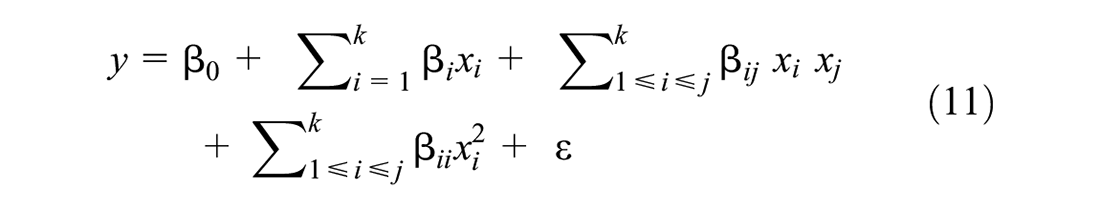
\begin{matrix} y = β_{0} + \sum_{i = 1}^{k} β_{i} x_{i} + \sum_{1 \leq i \leq j}^{k} β_{ij} x_{i} x_{j} \\ + \sum_{1 \leq i \leq j}^{k} β_{ii} x_{i}^{2} + ε \end{matrix}

(11)

where β₀ is the model constant and ε represents the residual associated to the experiments. Here, β_i, β_ij, β_ii are the coefficients for the linear, interaction, and quadratic terms, respectively.

Distress Model and Pavement Sections

ERAPave PP

ERAPave PP employs mechanistic-empirical design principles for the prediction of distresses in flexible pavements. For the prevailing environmental and traffic conditions, the tool primarily optimizes flexible pavements for fatigue cracking and rutting distresses. It can also analyze pavement structures for conditions that are typical of cold climates, such as frost heave and studded tire wear. Several studies that have been conducted using laboratory and APT investigations have shown that the pavement response and performance models of ERAPave PP are capable of delivering acceptable results ( 20 – 22 ).

The process that is used in ERAPave PP for the performance evaluation of flexible pavements is presented in Figure 1. As can be seen in Figure 1, the input module provides all the required information for pavement response and pavement performance evaluations. These inputs comprise mixture properties, structural inputs, environmental conditions, and traffic factors. A multi-layered linear elastic theory (MLET)-based analysis is used to determine the field variables, such as strain, stress, and deflection, for the prevailing pavement analysis condition ( 1 , 23 ). Damage is computed by the empirical component of the tool and this damage is accumulated on the basis of time or number of traffic cycles.

Figure 1.

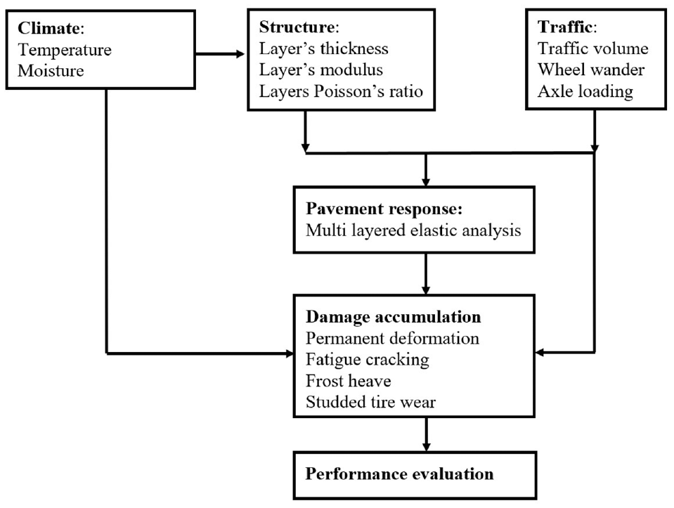
Flowchart for the ERAPave performance prediction tool.

ERAPave PP uses the layer strain approach for the prediction of rutting in flexible pavements. This approach obtains the total observed surface rutting by computing and aggregating the contribution of each layer ( 24 ). This requires separate models or model coefficients for the AC and unbound granular layers (UGLs). This is mainly because pavement structures are constructed using layers that have different material compositions. ERAPave PP takes into account the stress history dependence behavior of the material while computing the evolution of permanent deformation for each layer of the pavement structure. For this, a time-hardening approach that accounts for the stress path or stress level influence on permanent deformation accumulation is implemented ( 25 , 26 ).

Permanent Deformation Prediction for the Asphalt Concrete Layer

The permanent deformation behavior of the AC layers is affected by factors such as temperature, binder type and content, aggregate gradation, and structural thickness. Factors related to traffic are also observed to influence this behavior ( 11 ). ERAPave PP predicts the development and evolution of permanent deformation in the AC layers using the model that was originally developed for Pavement ME ( 4 , 27 ). The mathematical formulation of this model is presented in Equation 12. The model captures the permanent deformation behavior of the AC layers using factors such as traffic volume (N), temperature (T), and applied load level:

ε_{P} (N, T) = a T^{b} N^{c} ε_{r}

(12)

where ε_p and ε_r are the resilient and accumulated permanent strains, respectively. Here, a = 0.03, b = 1.85, and c = 0.27 are model coefficients

Permanent Deformation Prediction in Unbound Granular Layers

Permanent deformation or rutting is the primary failure mode for the layers that are comprised of unbound granular materials (UGMs). The permanent deformation behavior of these layers is highly dependent on factors such as structural thickness, traffic volume, stress level, stress history, moisture content, and aggregate gradation ( 28 – 30 ). ERAPave PP employs a strain-based model for the prediction of permanent deformation in layers such as the base, subbase, and SG ( 21 , 31 ). As can be seen in Equation 13, the model predicts permanent strain (ε_p) using as an input number of applied traffic cycles (N) and resilient strain (ε_r):

ε_{P} (N) = a N^{b (ε_{r})} ε_{r}

(13)

where a = 3.0 and b—which has values of 100, 200, and 250 for the base, subbase, and SG model coefficients, respectively.

Pavement Sections

This study was carried out using two APT sections. The studied sections (i.e., SE-14 and SE-18) represent different design features and are representative of Swedish in-service conditions. The sections were constructed using workmanship and equipment that are employed for the construction of actual field pavements. A schematic representation of the two sections is presented in Figure 2. As can be seen in Figure 2, the two structures consist of four distinct layers: a bituminous surface, a crushed aggregate base and subbase, and a sand SG, which is constructed over a rigid concrete floor.

Figure 2.

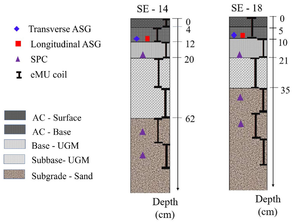
A cross-section view of the studied pavement sections.

As can be seen in Figure 2, the studied sections were embedded with sensors and gauges of different kinds. Instrumentation was provided in the longitudinal direction along the main loading path and a multiple set of sensors and gauges was provided for each variable of interest. The instruments provided a continuous measurement of the field variables for the whole testing period. For the measurement of the field variables, asphalt strain gauges (ASGs), soil pressure cells (SPCs), and vertical strain gauges (eMU coils) were provided. Measurements of interest were the longitudinal and transverse horizontal strains at the bottom of the AC layer, the compressive vertical pressure at different locations within the unbound and SG layers, and the full-depth vertical strain.

The APT facility is a fully insulated system where environmental factors such as moisture and temperature are fully controlled and continuously measured. Traffic loading is applied during the main accelerated loading stage using mobile HVS (Mark IV). The HVS is capable of applying different load levels and wheel configurations while moving at a speed of 12 km/h ( 20 , 22 ). The lateral application of the traffic in the transverse direction is also carried out during loading.

Surface rutting is measured using laser beams that are installed at five different locations along the longitudinal direction, while the permanent deformation of each layer is measured using the eMU coils. FWD measurements are performed on numerous occasions during construction and testing to assess the structure integrity of the pavement structure. It is also customary to perform surface elevation measurements that characterize the homogeneity of the structural thickness.

Table 1 provides the layer thickness and modulus of the individual layers for each APT section. These values represent average nominal conditions, and the moduli were calculated using average FWD measurements. For pavement response and performance calculations, the layer moduli obtained through the FWD were optimized further using the full-depth vertical strain measurements. This is required so that the material properties can reflect accurately the loading condition of the HVS. Testing was performed at a constant pavement temperature of 10°C while the moisture condition in the UGLs and SG was unaffected. During the main accelerated loading phase, the sections were subjected to a traffic loading that consists of single axles of different magnitudes and volumes. A dual wheel configuration with a tire pressure of 800 kPa was used for the traffic application. SE-14 was subjected in the first phase to 580,000 traffic cycles of 80 kN, while in the second phase 600,000 cycles of 100 kN were applied. For SE-18, the traffic was applied in three phases. Axle load magnitudes of 80, 100, and 120 kN, with traffic volumes of 481,000, 434,000, and 300,000 cycles, were applied during the three loading phases, respectively.

Table 1.

Nominal Layer Thickness and Modulus Values

APT section	Thickness (mm)			Modulus (MPa)
APT section	AC	Base	Subbase	AC	Base	Subbase	Subgrade
SE-14	120.0	80.0	420.0	5100.0	200.0	150.0	150.0
SE-18	100.0	100.0	150.0	5800.0	200.0	150.0	140.0

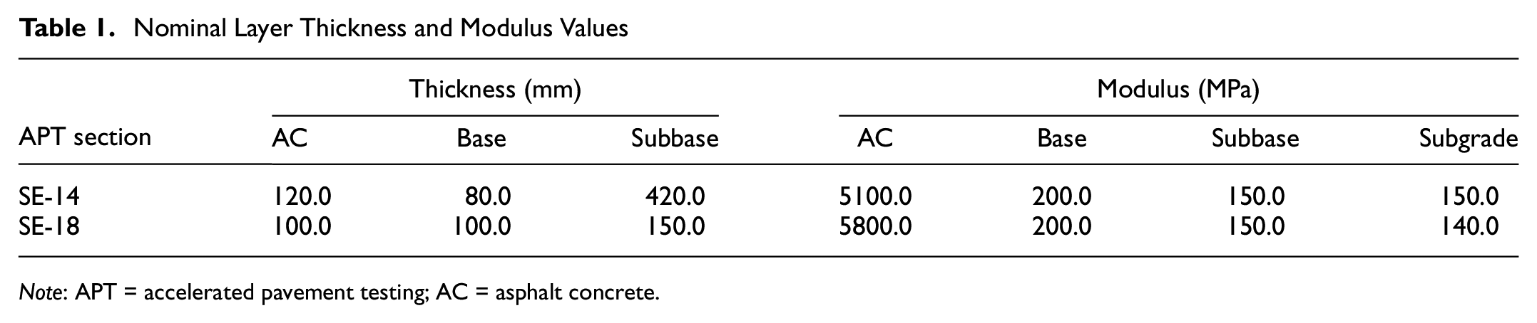
Note: APT = accelerated pavement testing; AC = asphalt concrete.

Results and Discussion

Variability Characterization

The design of pavement structures requires a multitude of inputs. As all of these inputs do not have the same level of impact on predicted performance, it will be uneconomical to consider all of them as random variables. A sensitivity analysis has shown that inputs related to traffic, environmental conditions, material properties, and structure influence significantly the rutting development in flexible pavements ( 11 ). As the APT was performed at a constant temperature and using a fixed volume and magnitude of traffic loading, the only inputs that are expected to be variable are the inputs related to the material and structure. Therefore, the thickness and modulus of each layer were modeled as random variables. The full probability approach, which uses a PDF along with the first and second moments of the data (i.e., mean sand standard deviation), was used to characterize the variability. In addition to the most common PDFs, such as normal and lognormal, PDFs such as Weibull, gamma, and general extreme value were used.

Layer Modulus

FWD testing were conducted using three dynamic load levels (30, 50, and 65 kN). The pavement response caused by the applied dynamic loads was received using geophones. As a variability study, multiple sets of testing were conducted along the longitudinal and transverse directions. All testing was conducted following the recommended guidelines and test protocols. Figure 3 provides the surface deflections for the load impact point along the longitudinal direction. As can be seen in Figure 3, a and b , these deflections show a remarkable variation, and this variation is consistent among the three dynamic loads.

Figure 3.

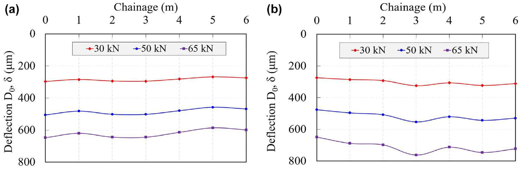
Longitudinal profile of the load impact point deflections for (a) SE-14 and (b) SE-18.

A backcalculation analysis that involves MLET-based analysis was employed to determine the modulus of each layer ( 32 ). To simplify the optimization and to reduce prediction error, the layers were grouped together to form a three-layered pavement structure: the AC, UGL, and SG. Furthermore, to eliminate the uncertainty associated with pavement thickness, the homogeneity of the structural thicknesses was carefully assessed. Table 2 presents the statistical analysis for each section layer modulus. As can be seen in Table 2, the SG is more homogenous than the asphalt and UGLs. The same pattern of variability was also observed in previously studied APT sections ( 12 ). However, for field sections, the AC and UGLs are more homogenous than the SG ( 6 ). For this study, coefficients of variation (CVs) of 20%, 15%, and 5% were selected to represent the variability associated with the AC, UGLs, and SG, respectively.

Table 2.

Layer Modulus Variability for the Studied Sections

Layer	Section	Minimum (MPa)	Maximum (MPa)	Mean (MPa)	Standard deviation (MPa)	CV (%)	PDF
AC	SE-14	4879.2	8715.0	6460.1	1090.6	16.9	Lognormal
AC	SE-18	3558.6	8699.8	6336.6	1385.2	21.9	—
UGL	SE-14	128.6	182.6	147.4	11.2	7.6	Lognormal
UGL	SE-18	90.1	233.3	186.4	29.9	16.0	GEV
Subgrade	SE-14	86.4	111.2	99.1	6.3	6.3	Lognormal
Subgrade	SE-18	94.4	109.4	99.9	3.9	3.9	Lognormal

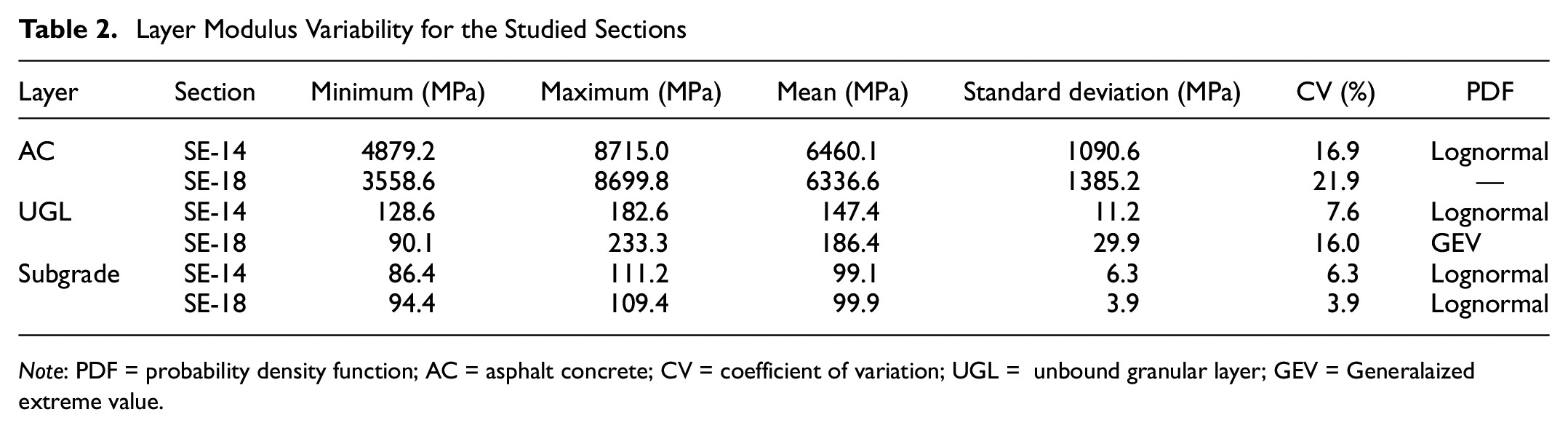
Note: PDF = probability density function; AC = asphalt concrete; CV = coefficient of variation; UGL = unbound granular layer; GEV = Generalaized extreme value.

The dispersion associated with the measured modulus was tested with various types of PDFs. Figure 4, a–f, presents the measured moduli of each layer fitted with a lognormal distribution. It is not uncommon for the measured modulus to be described and modeled concurrently by multiple PDFs. In addition, the sample size has a significant influence on the type of PDF that best fits the measurement. The histogram plots have also shown that the measured moduli of each layer exhibit a wide range of values. For this study, a lognormal PDF was selected to characterize the layer modulus variability.

Figure 4.

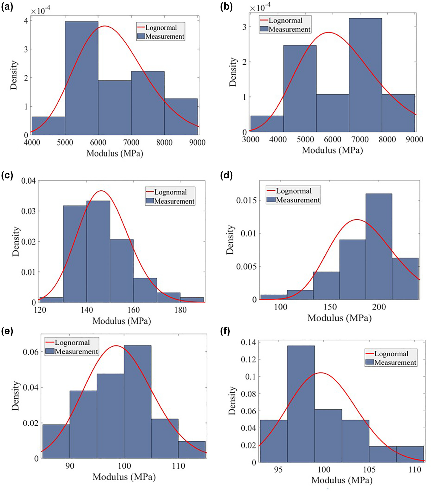
Modulus histogram fitted with a lognormal probability density function for SE-14 for the (a) asphalt concrete (AC), (c) unbound granular layer (UGL), and (e) subgrade, and for SE-18 for the (b) AC, (d) UGL, and (f) subgrade.

Layer Thickness

Elevation level measurements that characterize the uniformity of the compacted surface were carried out after the placement and compaction of each layer. As a variability study, multiple elevation level measurements were performed in both longitudinal and transversal directions. Figure 5 provides the center line average elevation level measurements for the longitudinal direction. As can be seen in Figure 5, a and b , there is a negative correlation between the layers. This is expected, as the intent during construction is to attain a smooth flat surface.

Figure 5.

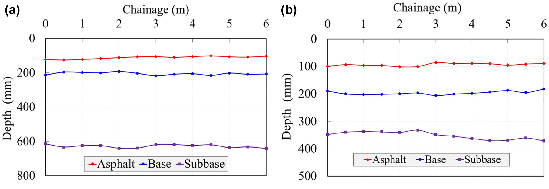
Longitudinal profile of the elevation level measurements for (a) SE-14 and (b) SE-18.

The thickness profile of each layer was obtained by deducting its elevation level from the layers adjacent to it. Table 3 presents the statistical analysis for each section layer thickness. As can be seen in Table 3, the CV for each layer falls within a narrow range, showing the consistent construction practice at the APT facility. For this study, CVs of 10%, 15%, and 10% were selected to represent the variability associated with the AC, UGL base, and UGL subbase, respectively.

Table 3.

Layer Thickness Variability for the Studied Sections

Layer	Section	Minimum (mm)	Maximum (mm)	Mean (mm)	Standard deviation (mm)	CV (%)	PDF
AC	SE-14	89.0	131.0	111.1	10.4	9.4	Normal
AC	SE-18	71.0	109.0	92.8	7.1	7.7	Normal
Base	SE-14	57.0	109.0	85.7	10.7	12.6	Normal
Base	SE-18	75.0	113.0	95.7	8.9	9.2	Weibull
Subbase	SE-14	393.0	457.0	427.8	18.9	4.4	Normal
Subbase	SE-18	125.0	181.0	152.7	15.0	9.8	Normal

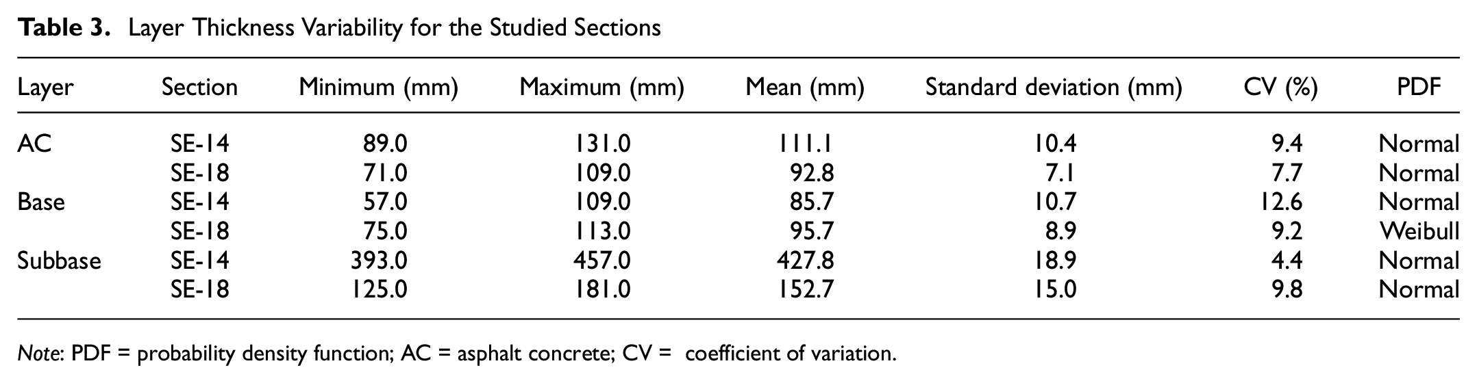
Note: PDF = probability density function; AC = asphalt concrete; CV = coefficient of variation.

Figure 6 presents the measured thickness of each layer fitted with a normal PDF for the two studied sections. As can be seen in Figure 6, a–f, the variability of layer thickness can be described by a normal PDF. The variability of the layer thickness was also observed as exhibiting a wide range of values. For this study, a normal PDF was selected to characterize layer thickness variability.

Figure 6.

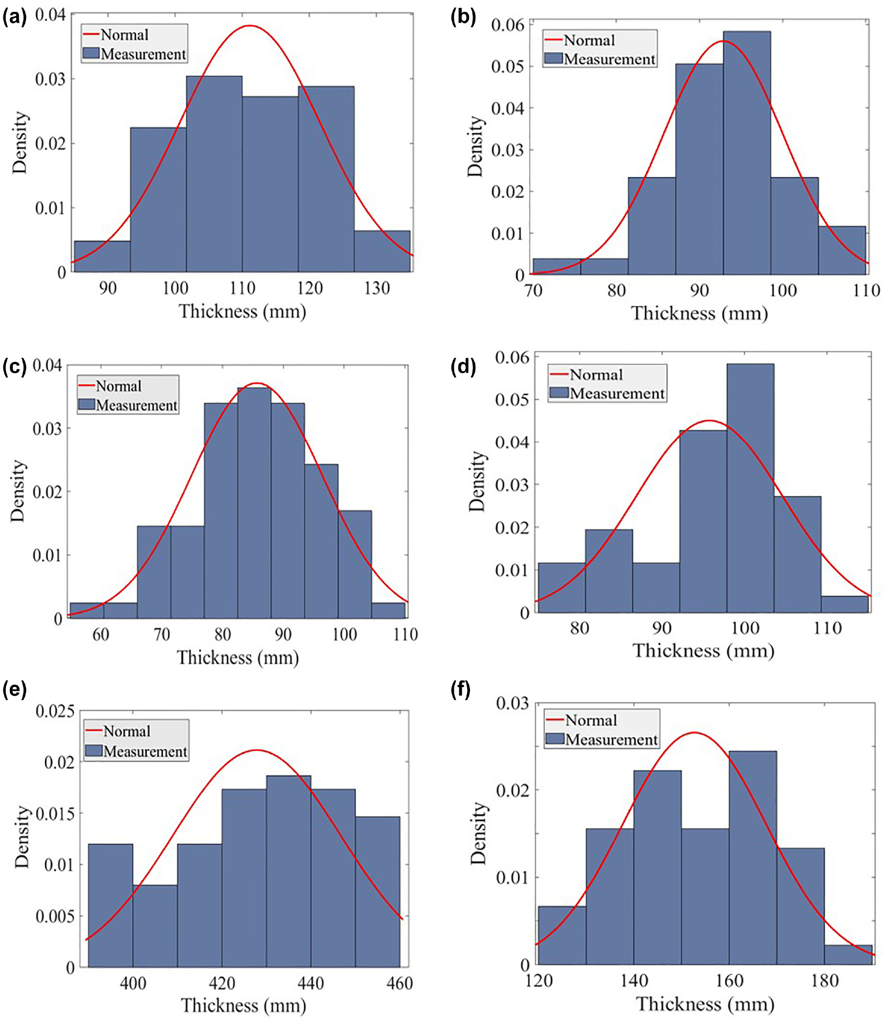
Thickness histogram fitted with a normal probability density function for SE-14 for the (a) asphalt concrete (AC), (c) base, and (e) subbase and for SE-18 for the (b) AC, (d) base, and (f) subbase.

Reliability Analysis

Predicted Rutting Variability

MCS was carried out to generate the frequency distribution of predicted surface rutting. As ERAPave PP requires a considerable amount of time to carry out many MCSs, the analysis was limited to 500 cycles. Although this number might not be enough to truly reflect the actual variability of predicted rutting, it will provide valuable insights with respect to the expected range of values. Statistical analysis has shown that a lognormal PDF with a CV range of 15%–30% can be used to describe the variability of the MCS-generated rutting. Figure 7 presents the MCS-generated rutting histogram fitted with a lognormal PDF for the two sections. The averaged measured value of the rutting is also included in the figures. As can be seen in Figure 7, a and b , there is an overlap between the measured average values and most frequent values generated by MCS, which shows the capability of the ERAPave PP rutting prediction model.

Figure 7.

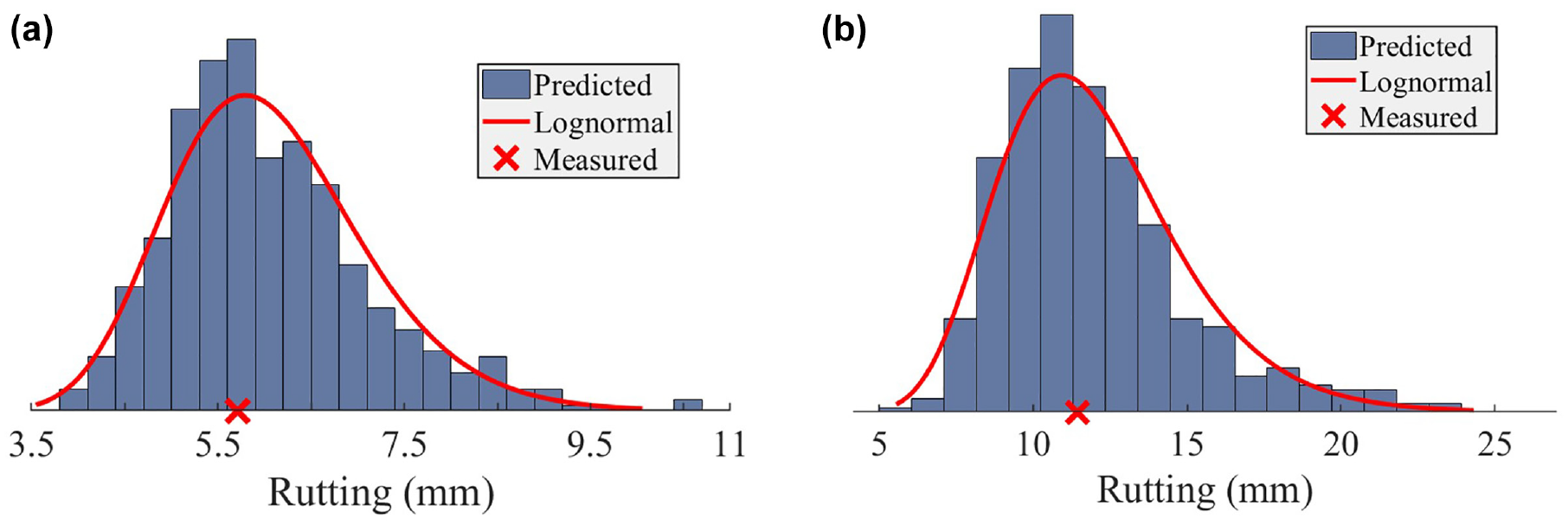
Monte Carlo simulation-generated rutting histogram fitted with a lognormal probability density function and measured values for (a) SE-14 and (b) SE-18.

Surrogate Model Validation

The CCD RSM generates the different level matrices using experiments that involve a full factorial design and an additional design where experimental points are at a certain distance from the center. This was achieved using the MATLAB inbuilt CCD function. A one-way analysis of variance (ANOVA), which was performed on 100 randomly generated experimental points, has shown that the generated surrogate models can deliver acceptable predictions. A direct comparison was also made between the rutting that was predicted by the actual and surrogate models. Figure 8 presents the comparison between the two values for the two studied sections. As can be seen in Figure 8, a and b , there is a good agreement between the two values. Coefficient of determination R² values of 0.94 and 0.87 were obtained for the surrogate models of SE-14 and SE-18, respectively. This shows the capability of RSMs in delivering results that are relatively accurate when appropriate methods and function types are used.

Figure 8.

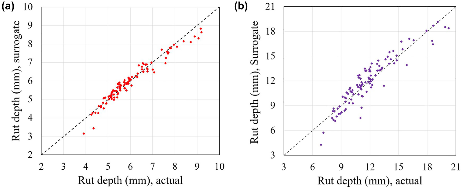
Comparison between actual and surrogate model predictions for (a) SE-14 and (b) SE-18.

Reliability Comparison

The limit state equation in Equation 3 was used to estimate the reliability of the two sections. As experimental sections that represent actual field conditions, the failure criteria for the two sections were established by carefully studying the existing guidelines and specifications. Thus, rut depths of 8 and 15 mm were established as failure criteria for sections SE-14 and SE-18, respectively. Two separate failure criteria were used for the two sections, as the sections represent different design and functional conditions.

The reliability of the two sections was assessed using the three approaches. In the first approach, MCS in conjunction with a surrogate model was used to determine the “exact” reliability of the two sections. MCS cycles of 10,000 were used, as this number of cycles was observed to be reasonable. The second approach utilizes the reliability methodology incorporated in Pavement ME. Equations 5–8 were used to determine the required SE for each layer and for the total observed surface rutting. The third approach estimates the reliability of the two sections using the FORM. Table 4 presents the estimated reliabilities according to the three approaches for the two sections.

Table 4.

Comparison of Estimated Reliability

Reliability analysis approach	Reliability (%)
Reliability analysis approach	SE-14	SE-18
MCS	96.1	81.8
Pavement ME	89.9	92.3
FORM	93.2	68.0

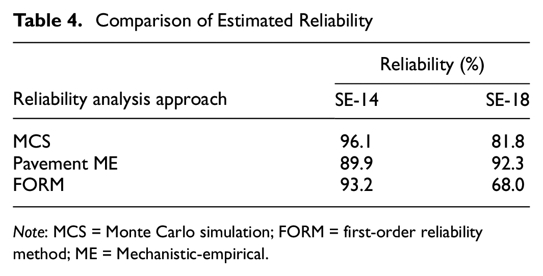
Note: MCS = Monte Carlo simulation; FORM = first-order reliability method; ME = Mechanistic-empirical.

As can be seen in Table 4, the estimated reliabilities of the three approaches differ significantly for both sections. The estimated reliabilities are more precise for SE-14 in comparison with SE-18. For SE-14, when compared with MCS, the reliabilities of Pavement ME and the FORM have normalized errors (NE) of 6.5% and 2.9%, respectively. For SE-18, these values are 12.9% and 16.8%, respectively. As can be seen in Figure 7b, the MCS-generated histogram of SE-18 exhibits a wide dispersion and might be the reason for the wide gap between the Pavement ME and FORM reliabilities.

In addition, for the Pavement ME approach, CV values of 29% and 23% were obtained for SE-14 and SE-18 rutting, respectively. This difference in CV values might be the reason why the Pavement ME approach delivered a higher reliability for SE-18 than SE-14. For the FORM approach, when compared with SE-14, the reliability estimate of SE-18 diverges by a significant margin from its corresponding MCS reliability. This might be attributed to the SE-18 surrogate model, which as can be seen in Figure 8b is less accurate and precise than the surrogate model in SE-14.

Conclusions

Reliability analysis approaches that rely on a probabilistic method of uncertainty propagation have not been fully utilized in pavement design. This is mainly attributed to factors such as the level of uncertainty associated with the pavement design process, the implicit nature of pavement performance evaluation, and the lack of accurate data on input variability. This has led to the adoption of simplified pavement reliability analysis methods that may not deliver the intended benefits. A comprehensive reliability analysis methodology that captures the combined variance of input variabilities on predicted performance is required. This would deliver designs of uniform performance, providing the right platform for the technical, economic, and environmental assessment of pavement structures.

The variability characterization of the APT sections has shown the challenge of obtaining uniform and homogeneous structures even in constructions that are performed in a controlled environment. The layer modulus and thickness of the APT sections exhibit less variation in comparison with field pavement sections. Unlike field sections, the SG of the APT structures is relatively uniform and homogenous than the AC and UGLs. Lognormal and normal PDFs can be used to describe the variability of the layer modulus and thickness, respectively. A lognormal PDF is also observed to be appropriate for describing the dispersion associated with MCS-generated rut depth.

The CCD RSM has managed to generate surrogate models that are relatively accurate, while the evaluated reliability analysis approaches are observed to provide reasonable estimates. The reliability estimates of the Pavement ME approach are highly dependent on the SE of each layer, as it lacks the mechanism to consider directly the variability associated with inputs. It is also observed that the currently utilized SE equations are positively skewed to higher rut depths, requiring further adjustments. MCS on the basis of a surrogate model can be a good alternative to obtain an “exact” estimate of the reliability, minimizing the forbidding computational time. As estimated “exact” values are highly dependent on the chosen number of simulated cycles, a further interpretation of these “exact” results is required. The FORM coupled with properly validated surrogate models can provide acceptable reliability estimates. In addition to reliability estimates, the FORM provides information on failure points and directional cosines of each random variable, making it preferable for the development of a deterministic reliability-based design procedure for pavement application.

Footnotes

Author Contributions

The authors confirm contribution to the paper as follows: study conception and design: Y. Dinegdae, S. Erlingsson; data collection: Y. Dinegdae; analysis and interpretation of results: Y. Dinegdae, A. Ahmed, S. Erlingsson; draft manuscript preparation: Y. Dinegdae, S. Erlingsson. All authors reviewed the results and approved the final version of the manuscript.

Declaration of Conflicting Interests

The author(s) declared no potential conflicts of interest with respect to the research, authorship, and/or publication of this article.

Funding

The author(s) disclosed receipt of the following financial support for the research, authorship, and/or publication of this article: This research was sponsored by the Swedish Transport Administration (Trafikverket).

ORCID iDs

Yared Dinegdae

Sigurdur Erlingsson

Data Accessibility Statement

The datasets generated during and/or analyzed during the current study are available from the corresponding author on reasonable request.

References

Huang

Pavement Analysis and Design. Prentice Hall, Upper Saddle River, NJ, 2004.

Santos

Ferreira

Life-Cycle Cost Analysis System for Pavement Management at Project Level. International Journal of Pavement Engineering, Vol. 14, No. 1, 2013, pp. 71–84. https://doi.org/10.1080/10298436.2011.618535.

American Association of State Highway and Transportation Officials. AASHTO Guide for Design of Pavement Structures. The Association, Washington, D.C., 1993.

ARA Inc. Guide for the Mechanistic-Empirical Design of New and Rehabilitated Pavement Structures. NCHRP 1-37A Final Report. ARA Inc., ERES Consultants Division, Champaign, IL, 2004.

Dinegdae

Y. H.

Birgisson

Reliability-Based Calibration for a Mechanics-Based Fatigue Cracking Design Procedure. Road Materials and Pavement Design, Vol. 17, No. 3, 2016, pp. 529–546. https://doi.org/10.1080/14680629.2015.1094397.

Timm

Newcomb

Birgisson

Galambos

Incorporation of Reliability Into the Minnesota Mechanistic-Empirical Pavement Design Method. Minnesota Department of Transportation. University of Minnesota, Department of Civil Engineering, Minneapolis, 1999.

Retherford

J. Q.

Mcdonald

Reliability Methods Applicable to Mechanistic-Empirical Pavement Design Method. Transportation Research Record: Journal of the Transportation Research Board, 2010. 2154: 130–137.

Dinegdae

Y. H.

Birgisson

Design Inputs Variabilities Influence on Pavement Performance Reliability. In Functional Pavement Design ( Erkens

Liu

Anupam

Yiqiu

, eds.), CRC Press, London, 2016, pp. 741–750.

Dinegdae

Y. H.

Birgisson

Reliability-Based Design Procedure for Fatigue Cracking in Asphalt Pavements. Transportation Research Record: Journal of the Transportation Research Board, 2016. 2583: 127–133.

10.

Timm

D. H.

Newcomb

D. E.

Galambos

T. V.

Incorporation of Reliability Into Mechanistic-Empirical Pavement Design. Transportation Research Record: Journal of the Transportation Research Board, 2000. 1730: 73–80.

11.

Maji

Das

Reliability Considerations of Bituminous Pavement Design by Mechanistic-Empirical Approach. International Journal of Pavement Engineering, Vol. 9, No. 1, 2008, pp. 19–31. https://doi.org/10.1080/10298430600997240.

12.

Kenis

Wang

Pavement Variability and Reliability. Proc., 5th International Symposium on Heavy Vehicle Weights and Dimension, HVWD5, No. 202, Maroochydore, Queensland, Australia, Part 3, Conference Organising Committee (C/- Roaduser Research), Melbourne, Australia, 1998, pp. 213–231.

13.

Louw

Jones

Lessons Learnt From Accelerated Pavement Testing of Full-Depth Recycled Material Stabilized With Portland Cement. In Accelerated Pavement Testing to Transport Infrastructure Innovation ( Chabot

Hornych

Harvey

Loria-Salazar

, eds.), Springer, Cham, Switzerland, 2020, pp. 309–318.

14.

Harvey

Popescu

Accelerated Pavement Testing of Rutting Performance of Two Caltrans Overlay Strategies. Transportation Research Record: Journal of the Transportation Research Board, 2000. 1716: 116–125.

15.

Divinsky

Ishai

Livneh

Probabilistic Approach to Pavement Design Based on Generalized California Bearing Equation. Journal of Transportation Engineering, Vol. 124, No. 6, 1998, pp. 582–588.

16.

Dinegdae

Onifade

Birgisson

Lytton

Little

Towards a Reliability-Based Pavement Design Using Response Surface Methods. Transportation Research Record: Journal of the Transportation Research Board, 2018. 2672: 97–107.

17.

Rackwitz

Fiessler

Structural Reliability Under Combined Random Load Sequences. Computers and Structures, Vol. 9, No. 5, 1978, pp. 484–494.

18.

Hasofer

A. M.

Lind

N. C.

An Exact and Invariant Second-Moment Code Format. Journal of Engineering Mechanics Dvision, Vol. 1, No. 100, 1974, pp. 111–121.

19.

Montgomery

Design and Analysis of Experiments: Response Surface Method and Designs. John Wiley & Sons, Hoboken, NJ, 2005.

20.

Ahmed

A. W.

Erlingsson

Evaluation of Permanent Deformation Models for Unbound Granular Materials Using Accelerated Pavement Tests. Road Materials and Pavement Design, Vol. 14, No. 1, 2013, pp. 178–195. https://doi.org/10.1080/14680629.2012.755936.

21.

Dinegdae

Erlingsson

Evaluation of Permanent Deformation Models for Flexible Pavements Using Accelerated Pavement Testing. In Accelerated Pavement Testing to Transport Infrastructure Innovation ( Chabot

Hornych

Harvey

Loria-Salazar

, eds.). Lecture Notes in Civil Engineering, LNCE, Vol. 96, Springer, Cham, Switzerland, 2020, pp. 399–408. https://doi.org/10.1007/978-3-030-55236-7_41.

22.

Saevarsdottir

Erlingsson

Carlsson

Instrumentation and Performance Modelling of Heavy Vehicle Simulator Tests. International Journal of Pavement Engineering, Vol. 17, No. 2, 2016, pp. 148–165. https://doi.org/10.1080/10298436.2014.972957.

23.

Erlingsson

Ahmed

A. W.

Fast Layered Elastic Response Program for the Analysis of Flexible Pavement Structures. Road Materials and Pavement Design, Vol. 14, No. 1, 2013, pp. 196–210. https://doi.org/10.1080/14680629.2012.757558.

24.

Barksdale

R. D.

Laboratory Evaluation of Rutting in Base Course Materials. Presented at the Third International Conference on the Structural Design of Asphalt Pavements, Grosvenor House, London, September 11–15, 1972.

25.

Lytton

R. L.

Uzan

Fernando

E. G.

Roque

Hiltumen

Stoffels

S. M.

Development and Validation of Performance Prediction Models and Specifications for Asphalt Binders and Paving Mixes. Strategic Highway Research Program, National Research Council, Washington, D.C., 1993.

26.

Erlingsson

Rahman

M. S.

Evaluation of Permanent Deformation Characteristics of Unbound Granular Materials by Means of Multistage Repeated-Load Triaxial Tests. Transportation Research Record: Journal of the Transportation Research Board, 2013. 2369: 11–19.

27.

Ahmed

A. W.

Erlingsson

Evaluation of a Permanent Deformation Model for Asphalt Concrete Mixtures Using Extra-Large Wheel-Tracking and Heavy Vehicle Simulator Tests. Road Materials and Pavement Design, Vol. 16, No. 1, 2015, pp. 154–171. https://doi.org/10.1080/14680629.2014.987311.

28.

Tseng

K.-H.

Lytton

R. L.

Prediction of Permanent Deformation in Flexible Pavement Materials. In Implication of Aggregates in the Design, Construction, and Performance of Flexible Pavements ( Schreuders

H. G.

Marek

C. R.

, eds.), ASTM STP 1016, American Society for Testing and Materials, Philadelphia, PA, 1989, pp. 154–172.

29.

Erlingsson

Impact of Water on the Response and Performance of a Pavement Structure in an Accelarated Test. Road Materials and Pavement Design, Vol. 11, No. 3, 2010, pp. 863–880. https://doi.org/10.3166/rmpd.11.863-880.

30.

Lekarp

Dawson

Modelling Permanent Deformation Behaviour of Unbound Granular Materials. Construction and Building Materials, Vol. 12, No. 1, 1998, pp. 9–18. https://doi.org/10.1016/S0950-0618(97)00078-0.

31.

Rahman

M. S.

Erlingsson

Ahmed

Dinegdae

A Model for the Permanent Deformation Behavior of the Unbound Layers of Pavements. Proc., 11th International Conference on the Bearing Capacity of Roads, Railways and Airfields, Vol. 1, CRC Press, London, 2022, pp. 277–287. https://doi.org/10.1201/9781003222880-25.

32.

Ullidtz

Overlay and Stage by Stage Design. Proc., 4th International Conference on Structural Design of Asphalt Pavements, Vol. I, Ann Arbor, Michigan, University of Michigan, Ann Arbor, August 22–26, 1977, pp. 722–735.

Toward a Comprehensive Pavement Reliability Analysis Approach

Abstract

Keywords

Objective

Pavement Reliability

Reliability Methods

Pavement ME Reliability

Monte Carlo Simulation

The First-Order Reliability Method

Distress Model and Pavement Sections

ERAPave PP

Permanent Deformation Prediction for the Asphalt Concrete Layer

Permanent Deformation Prediction in Unbound Granular Layers

Pavement Sections

Results and Discussion

Variability Characterization

Layer Modulus

Layer Thickness

Reliability Analysis

Predicted Rutting Variability

Surrogate Model Validation

Reliability Comparison

Conclusions

Footnotes

Author Contributions

Declaration of Conflicting Interests

Funding

ORCID iDs

Data Accessibility Statement

References