
Abstract
Road infrastructure plays an important role in the economic and social development of societies. Thus, it requires effective and timely responses to cope with and embrace uncertain future changes. This study proposes an integrated, scenario-based strategic model which estimates transport demand, network performance, emission, and energy consumption. The model accounts for future economic, behavioral, policy, and technological developments by including four future scenarios and traces the possible changes in transport infrastructure performance. It primarily aims at supporting infrastructure decisions by quantifying a set of network and environmental performance indicators along their spatial–temporal dimension. Moreover, the effects of transport demand and energy transition policies on road performance are considered within each scenario. This model is applied in a case study region covering the main industrial and urban regions of the Netherlands. The discussed results provide insights into the possible infrastructure investments within each scenario and elaborate on the possible effects of policies.
Keywords
There is an increasing investment need in many countries to keep infrastructure assets at desired performance levels and ensure national and regional economic prosperity and social welfare ( 1 , 2 ). Infrastructure investments are capital-intensive and have long-lasting environmental and socio-economic impacts. Thus, identifying required investments along their temporal and spatial dimension becomes crucial for allocating limited resources in a way that future challenges such as climate change, urbanization, and technological advancements are being addressed ( 3 ). Related to this, transportation road networks have the highest share in freight and passenger transport ( 4 ) and are one of the main sources of greenhouse gas emissions. Understanding the effects of economic, political, social, and technological changes on the performance of road networks will thus support decision-making on future-relevant infrastructure investments.
Modeling the performance of road infrastructure can provide these insights on which decision-makers can make judgments under plausible scenarios and identify required measures to attain desired performance levels ( 5 , 6 ). Performance modeling becomes more useful when it allows the evaluation of different performance aspects such as capacity utilization, energy consumption, and emissions. However, identifying the future conditions of road infrastructure operation remains challenging because of the high uncertainties associated with future changes ( 7 ). To account for these uncertainties, typically several possible future scenarios are assumed to explore performance implications and the array of potential responses. By combining quantitative and qualitative data illustrative future images can be constructed for plausible pathways ( 8 ).
The literature in infrastructure investment planning provides us with examples of performance modeling under different future scenarios for road networks. These include performance analyses focusing on either passenger transport (e.g., de Bok et al. [ 9 ]), freight transport (e.g., Ambrosini et al. [ 10 ]), or emission and energy demand arising from road transport (e.g., Krause et al. [ 11 ]). Such analyses can also be found in national transport models, like the Dutch National Model System (LMS) ( 12 ). An example that combines freight and passenger modeling is TRANS-TOOLS (“TOOLS for TRansport Forecasting ANd Scenario testing”). This is a scenario-based transport network model to evaluate the European-level -NUT3- transport policies ( 13 , 14 ). However, scenario-based performance analyses of road infrastructure that integrate several performance parameters are scarce. To the best knowledge of the authors, there are only a few examples that estimate traffic demand and the consequences for energy consumption and environmental emission under different scenarios. PRIMES-TREMOVE is a simulation transport model that estimates future passenger and freight demand, energy consumption, and emissions for a reference case for EU member-states ( 15 ). Although the model projects the evolution of demand for passenger and freight transport, it does not account for uncertainties in future pathways. Moreover, it does not address infrastructure performance resulting from a certain future demand. The German Aerospace Center’s (DLR) “Transport and the Environment” project does include freight and passenger models for future mobility trends as well as emission and energy demand models to trace the transportation impacts on people and the environment ( 16 ). Freight models are based on a regression analysis of the gross-added value of different economic sectors including transport costs and time effects ( 17 ). Passenger models follow the four-step transport modeling approach and estimate short- and long-distance transport demand considering population composition, trip travel time, and costs ( 18 ). Projected emission and energy consumption factors enable estimation of the environmental effects of transport given three future scenarios addressing specific policy and technological development trajectories ( 19 ). The models provide a fine-scale analysis of disaggregated economic and demographic data. However, the scenarios are limited in their anticipatory power, as they assume similar population and wealth development and distribution. The Multi-Scale Infrastructure Systems Analytics (MISTRAL) model of the Infrastructure Transitions Research Consortium (ITRC) ( 20 , 21 ) is based on the National Infrastructure Systems Model (NISMOD) and provides an integral modeling of freight, passenger, emission, and energy demand to inform strategic infrastructure decision-making. It allows flexible scenario-based estimation of transport demand, emission, and energy. However, the model is limited in major demand determinants for a better understanding of future demand and performance of road infrastructure. For instance, the effect of remote working on transport demand can provide a more distinct picture of the possible future road performance. The effect of the economic structure on freight demand with an increasing share of the service sector can generate further insights in future transport demand. Furthermore, technological development and diffusion in automotive and energy production industries can reduce well-to-wheel transport emissions. These emission factor improvements under different scenarios can have an influence on the future environmental performance of the transport sector. Although fuel efficiency improvements have been considered, transport emission factor enhancements have not yet been addressed.
Given the shortcomings of previous research, the main objective of this paper is the development of an integrated, scenario-based strategic model that not only estimates freight and passenger road transport demand under distinct future scenarios but also projects infrastructure network performance as well as demand impacts under these scenarios. More specifically, we develop incremental demand estimation models for the study of future road network performance developments. Compared with existing elasticity-based strategic transport models our models are more comprehensive by including additional main demand determinants, such as the effects of vehicle ownership and remote working on passenger demand, as well as the effects of international trade and the growth of the service sector in the economy on the freight transport demand. Moreover, the change in emission and energy consumption factors over time is addressed in line with assumed future technological developments. Here, four future scenarios are adopted from the work of Neef et al. ( 22 ). The behavioral, socio-economic, policy-related, and technological dimensions of these scenarios are reflected in the model. The scenarios span to 2050 and were developed for the context of the Netherlands through a novel hybrid approach comprising document analysis and disaggregative policy Delphi. Introducing these scenarios increases the anticipatory power of our model as they enable the exploration of changes in the set of infrastructure demand factors based on plausible narratives about the future. Different levels of road performance can be estimated in relation to capacity utilization, delay, emission, and energy consumption by considering the uncertainties of demand-relevant future developments in a coherent and consistent way ( 7 ). As such, the proposed model will be able to support infrastructure planning by answering the question: what road infrastructure demand and performance can be expected under future pathways? The decision-support potential of the model not only stems from the flexible analysis of distinct future scenarios including a comprehensive set of main demand determinants. It is also based on suitability for national and regional analysis and its low computation run time.
The model is implemented in a region which covers the most important industrial and urban areas of the Netherlands. This region represents a suitable case for integrated performance analysis, because of its high spatial density, the high investment needs because of aging infrastructure, and infrastructure networks functioning at a near-capacity state. The proposed model aims, in the first instance, to support road asset managers and owners in investment-related decisions by tracing the effect of certain future trends on the performance of infrastructure. By exploring the possible demand and performance development trajectories through relevant performance indicators, the model supports investment planning in identifying required responses—such as parts of the network with high congestion levels. Second, the performance effect of certain policies inherent in future scenarios—for example, the effect of encouraging remote working on road network congestion—can be revealed. This further clarifies the potential implications of demand management, pricing, and systems’ efficiency enhancements. Therefore, the proposed model can be used for assessing infrastructure investment and identifying policy implications under uncertain futures. Its low computation time enables quick and numerous analyses.
In the next section, the model design and components are introduced. Following this we describe the case study scope, used data, and scenario adaptations. We continue by presenting and discussing the results, and concluding remarks are provided in the final section.
Model Design
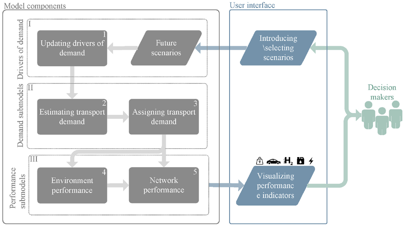
The proposed model (Figure 1) aims to reveal the changes in the performance of road transport infrastructure under future scenarios. It consists of infrastructure demand submodels estimating freight and passenger transport demand, infrastructure performance submodels estimating capacity utilization, emission, and energy consumption as a consequence of transport demand, and demand drivers based on a set of plausible future scenarios. To give decision-makers the possibility to select scenarios and analysis periods and to provide visualized feedback on modeling results, a user interface is connected to the model engine. Decision-makers are assisted in making more informed investment decisions and tracing the effect of a spectrum of policy measures (e.g., demand management, pricing) included in the scenarios on road transportation demand and performance.
Model overview.
Future Scenarios
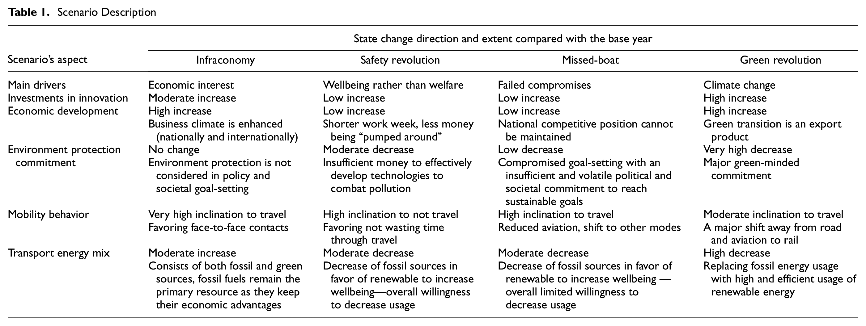
Four future scenarios from the work of Neef et al. ( 22 ) (referred to as the core scenarios) were adapted to provide quantitative inputs for the considered determinants of passenger and freight transport demand. Socio-economic variables, world trade, and fuel price are the main determinants of transport demand defined by different scenarios. Additionally, the scenarios address different future pathways of behavioral, climate, and technological changes. A behavioral change that affects transport demand is the shift toward more remote working in the aftermath of the COVID-19 pandemic ( 23 ). The degree of adaptation and mitigation efforts to respond to climate change such as pricing of fuel also affects transport demand and eventually CO2 and NOx emissions. To account for possible technological transitions and advancements, different levels of the future fuel mix (i.e., fossil, electricity, and hydrogen), as well as variations in the load factor are considered under different scenarios ( 24 ). In Table 1, the different aspects of the scenarios are summarized. There is a core driving force in each scenario around which a future pathway is shaped. That helps in understanding the developments to be expected from different aspects of the future scenarios. The innovation aspect of the scenarios covers expected technological advancements, which can affect road network performance (e.g., lower energy consumption and emission). Economic development has a noticeable impact on both passenger and freight demand as a result of increased economic activities. The level of commitment within each scenario in relation to the environmental protection measures is another important aspect that affects emission and energy demand arising from road network transport. Such a commitment can facilitate budget assignments and required shifts in institutional, technological, political, and social environments to respond sufficiently to environmental challenges. Thus, through the degree of commitment of each scenario, we can include plausible projections for the variables (e.g., emission factor developments) that affect road network emission and energy consummation. The mobility behavior included in this paper is limited to remote working, which can affect the transport need and congestion, thus, the road network performance. Finally, the energy mix used in transport differs for each scenario and is aligned with the innovation, economic development, and environmental protection commitment levels. This aspect can explore the degree of energy transition toward cleaner energy sources. The following paragraphs provide the core scenario description.
Scenario Description
Core Scenarios’ Description
Green Revolution
The Green Revolution represents an environmentally friendly future with a drastic reduction in the use of fossil energy and emission. Policy measures are directed toward reaching the climate goals set in the Paris Agreement. Much will be invested in energy transition; thus, environmentally friendly technologies will be extensively adopted with a high societal acceptance for a less polluting lifestyle. This includes a high level of remote working facilitated by technological developments required for secure and satisfactory distant working. Moreover, polluting energy resources are taxed to encourage a transition toward cleaner resources.
Infraconomy
The Infraconomy envisions a future in which economic interests act as the driving force. That results in strong product-based economic developments and the dependency on fossil energy. Liberal market mechanisms favor no energy resource in providing them with tax advantages. Globalization continues at a high pace with an increase in global trade. Much will be invested back in constructing and expanding infrastructures—with more focus on road—rather than investing in research and development. Face-to-face business meetings are valued more. Limited efforts will be put into tackling the climate crisis. However, some developments such as the limited modal shift to waterways—proportional to the growth of the port companies—reduce emissions.
Missed-Boat
The Missed-Boat scenario envisions a future based on failed compromises to impose policy measures directed toward climate change. This future will leave us with different environmental, societal, political, and governance-related challenges, which causes failure in the attempts to reach a more sustainable society. Environmentally friendly technologies will be adopted to a limited extent. Fossil energy will remain the main source of energy, and global trade will be affected by protectionism and political conflicts.
Safety Revolution
Under the Safety Revolution scenario, wellbeing is the central driver. People tend to work less, more meetings will take place virtually, the use of less polluting means of transport will increase, population growth in rural areas will be higher than in dense urban areas, and there will be reduced achievement of environmental goals because of slow economic growth. A more conscious lifestyle will result in more consumption of local goods. This trend, in addition to low economic growth, leads to a reduction in world trade. Furthermore, low research and development budgets resulting from low economic growth decrease investments in new technologies and energy transition. Despite the social acceptance of remote working, widespread, reliable, and secure remote working infrastructure will not be available.
Transport Demand Submodels
We propose two transport demand submodels for estimating passenger and freight transport demand of roads. An incremental demand modeling approach forms the basis of these submodels. This approach is suitable for developing models for strategic transport planning, as it reduces the efforts for data collection and processing, as well as being more communicable concerning the model features and results ( 25 ).
The product incremental function proposed by Lovrić et al. (
20
) is adopted in our study. The product incremental function is an elasticity-based formulation and includes sets of endogenous and exogenous variables which influence the trip generations and attractions in the origin and destination zones (
Passenger Demand at the Road Network
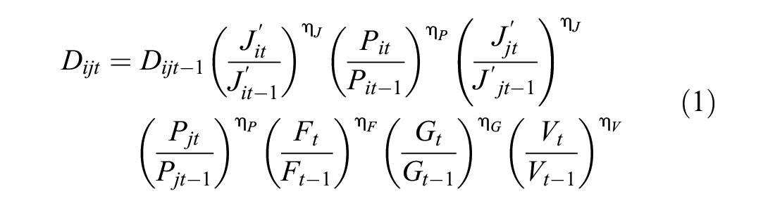
Income, car ownership growth, population size, labor participation, and fuel price as the main demand determinants of road transport that can be used to estimate future demand to a great extent (
26
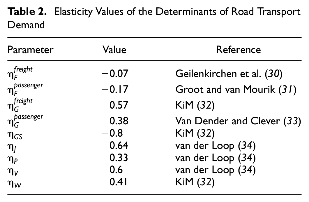
). Therefore, the road demand estimation submodel (Equation 1) covers these main determinants and makes use of the most recent elasticity values relevant to the Netherlands’ context. The elasticity values presented in Table 2 are based on literature review and policy documents from the Netherlands, which are specific to socio-economic and geographical characteristics of the case presented in the case study. They are represented by a column vector

GDP per capita is used as a proxy for income per capita, which follows a similar trend in high-income countries ( 27 ) because the elasticity of the income per capita is not known in the Netherlands. Typically, the GDP and the number of vehicles are correlated, as the former is the most important determinant of car ownership ( 28 ). However, in the Netherlands, income does not have a strong effect on vehicle ownership, compared with other high-income countries. One reason is the Dutch bike culture. Furthermore, passengers with higher income consider traveling with trains as a luxury service ( 29 ). Consequently, we included both variables for the road demand estimation.
Elasticity Values of the Determinants of Road Transport Demand
Freight Transport Demand
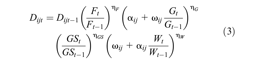
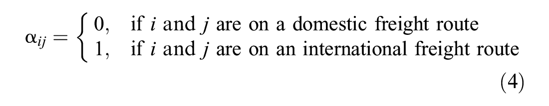
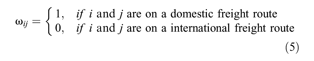
Among a wide range of determinants that influence freight transport demand, such as economic and logistical structure ( 35 ), Knoope and Francke ( 36 ) identified GDP change in different sectors and the world trade index as most influential on freight demand in the Netherlands. In this submodel, we include the long-term effect of the GDP change and the GDP share of the service industry. The former represents economic activities from which freight demand arises. The latter addresses the economic switch toward the service industry, which has less freight demand compared with production-based industries. The world trade index as an indicator of globalization is also considered, which leads to an increase in international freight transported ( 37 ). Additionally, transport time and prices determining transport costs are included in the freight demand estimation. Although the effect of these determinants can be lower compared with other determinants ( 36 , 38 ), they can trace the effect of competition between transport modes. Moreover, the dependency on the energy sector can be considered by taking fuel prices into account. Equation 3 estimates the freight road demand.
Infrastructure Performance Submodels
We consider environmental and network performance indicators in two performance submodels (see Table 3).
Model Indicators
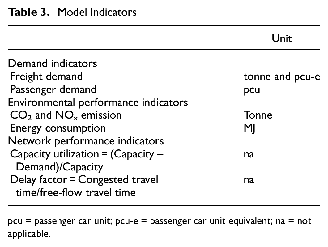
pcu = passenger car unit; pcu-e = passenger car unit equivalent; na = not applicable.
Network Performance Indicators
Capacity utilization and delay factor are the main indicators of road network performance. The former indicates the utilized capacities of the road trunks. The latter represents the ratio between the congested travel time and the free-flow travel time in traffic situations with no congestion. To determine the congested travel time, the estimated traffic demand is assigned to the road network. We follow a capacity-restraint traffic assignment approach which is mostly used in strategic transport planning ( 39 ). To implement this approach, the volume–delay function (VDF) proposed by the Bureau of Public Roads is used (Equation 6) that is very popular because of its simplicity of the mathematical form and the minimum input requirements ( 40 ). A passenger car unit equivalent of 2 for each truck is considered, as proposed by Webster and Elefteriadou ( 41 ).

where
Environmental Performance Indicators
Transportation is one of the main sources of CO2 and NOx which contributes to climate change, imposes health risks, and adversely affects nature and biodiversity. Road transport emission and energy consumption are calculated bottom-up using variable flows, emission, and energy consumption factors. Equations 7 to 9 calculate the energy demand and emission resulting from freight and passenger transport.
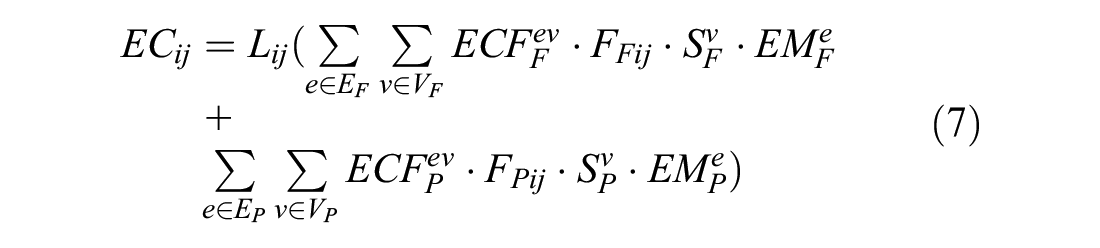
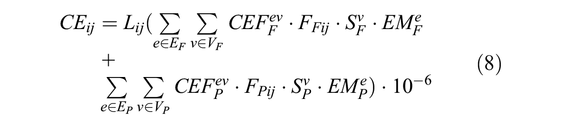

where
Freight Transport Fleet and Emission Factors at the Base Year (Diesel)
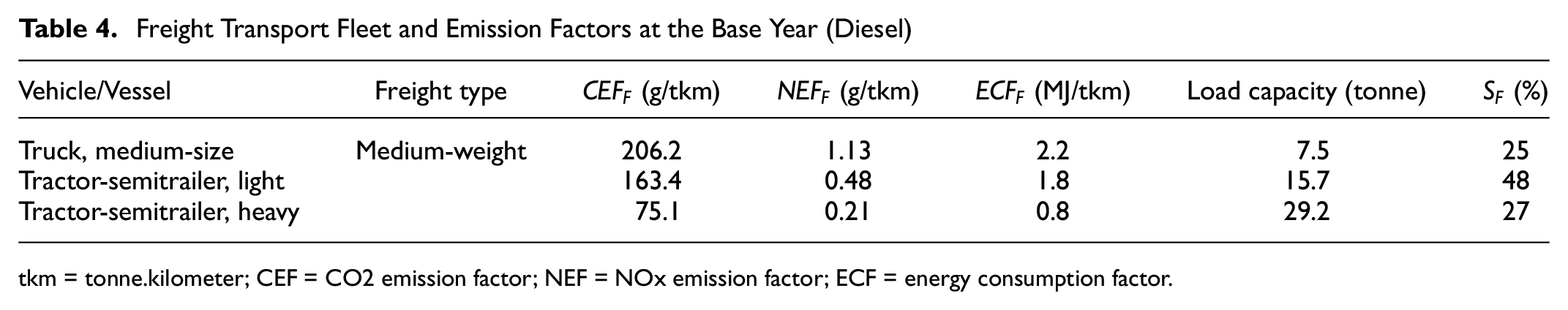
tkm = tonne.kilometer; CEF = CO2 emission factor; NEF = NOx emission factor; ECF = energy consumption factor.
Passenger Transport Fleet and Emission Factors at the Base Year (Petrol)
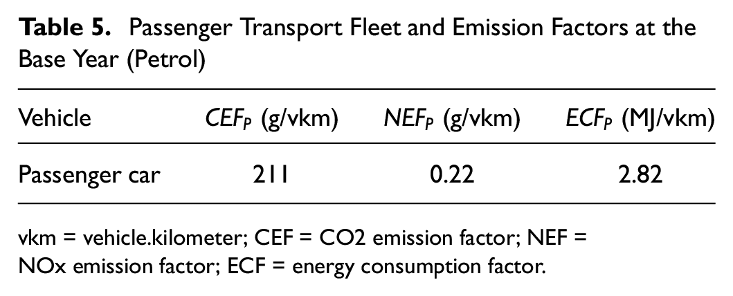
vkm = vehicle.kilometer; CEF = CO2 emission factor; NEF = NOx emission factor; ECF = energy consumption factor.
The described submodels in the Model Design section are implemented in the MOVICI simulation platform, which facilitates simulation, as well as communication and analysis of results ( 49 ).
Case Study
Scope
The case study region (see Figure 2) covers the three Dutch provinces of Noord-, Zuid-Holland, and Utrecht. The region is the most populated in the Netherlands with more than 8 million inhabitants (around 50% of the total population). Moreover, the two biggest ports of the Netherlands (Rotterdam and Amsterdam) are located in this region, making the region economically important for national and international businesses. Two major European railway routes (Trans-European Network for Transport), a part of the Betuweroute, and major waterways such as Hollandse Diep and Amsterdam-Rijnkanaal pass through the region. Because of the economic and social importance of the region, it is a suitable case to implement the proposed model and generate insights that are of interest to policymakers and infrastructure agencies.
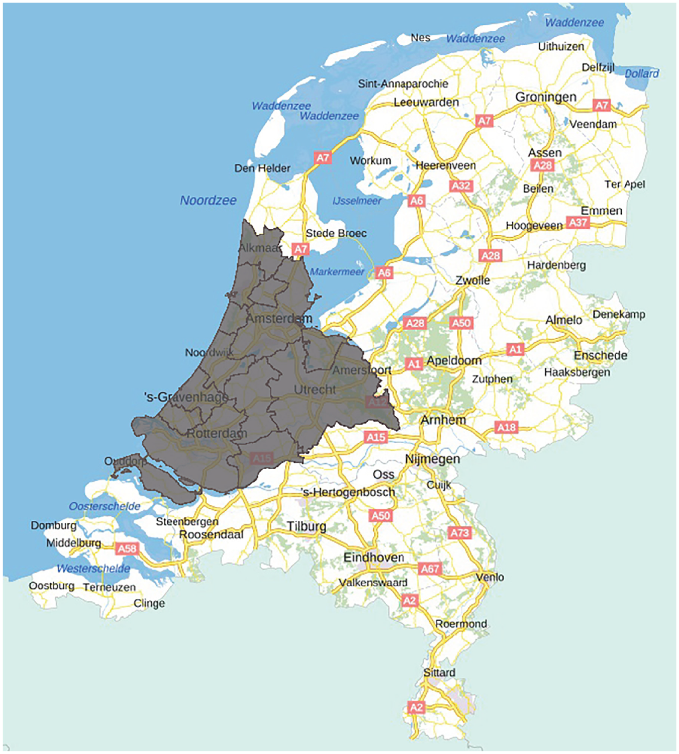
Case study region.
Municipalities represent the spatial aggregation level. Road infrastructures included are the main highways (named A-roads) and national roads (named N-roads). They fall under the responsibility of Rijkswaterstaat, the agency that designs, constructs, manages, and maintains the main road and water infrastructure in the Netherlands. Road Infrastructure is represented by sets of nodes and links. Polygons indicate geographical and administrative boundaries.
The base year is 2019, which was selected to avoid possible data distortions as a result of the COVID-19 pandemic in 2020 and 2021. The time horizon is 2050 with a time step of one year. Demand was estimated for the extended evening peak hours from 16:00 to 20:00, which is the most congested period of a day, mainly because of the overlapping work–home and leisure trips ( 50 ).
Data
Collected data were categorized into infrastructure attributes, entities, and traffic measurements. Infrastructure attribute data include the attributes that were necessary to estimate and distribute demand (e.g., the number of road lanes, etc.), and set the traffic constraints (e.g., capacities, maximum speeds, etc.). Entity data consist of demand nodes and highway links including their geometry and location. Demand nodes were determined by extracting the extremities of the road network links at the entrance and exit points of highways. In this manner, the most complete set of traffic measurement points became available to be used to estimate the base year passenger OD (see section Base Year OD Matrices). Additionally, to create an open network, seven external demand nodes were considered at the centroids of the Netherlands’ NUTS3 regions (European Nomenclature of Territorial Units for Statistics level 3). This level of geographical subdivision divides the country into regions finer than provinces but coarser than municipality boundaries and is used for statistical purposes (e.g., transport demand). The demand nodes represent national and international destinations for passenger and freight transport. Traffic measurement data cover the most recently observed intensities, speeds, and travel time for the road network. This set of data was used to derive the base year OD matrices.
The main data sources were open-source national databases, and data sets acquired by infrastructure owners (Port of Rotterdam and Rijkswaterstaat), and Statistics Netherlands (CBS) ( 51 – 53 ). Entity data and most of the infrastructure attribute data are complete and yearly updated. This includes data on the number of lanes, maximum speed, geometry, and location of road network links and network connectivity. The data sources missed link capacities, which were derived based on the number of lanes and guidelines provided by Transportation Research Board ( 54 ). Traffic measurement data contain average observed travel time, speed, intensity, vehicle type (by length), and observation location, which gets updated regularly. The data set covers more than 90% of the observation points of the case study region. Data sets including freight flows for each modality contain complete aggregated flows among national and international regions of the case study region. Statistics Netherlands (CBS) maintains these data sets. Because of their completeness and regular update, we regard the used data sets as of sufficient quality for our analysis. The collected data were processed using QGIS, Python scripts, and manual inspection, and this processing can be summarized as aggregating the data instances to a suitable spatial resolution, cleaning, connectivity check, deriving the base year demand and performance data, deriving the transport demand nodes, connecting attribute and performance information to the spatial data layers and simplifying the data instances.
Assignment VDF Calibration
We calibrated the assignment VDF Equation 6, which led to 0.64 and 4 for
In total, 995 measurement points for the road links with multiple lanes were used in the calibration. The estimated parameters in Equation 3A resulted in a root mean square error (RMSE) of 7.39. The data set without outliers yielded an RMSE of 3.27. Some 80% of the measurement point data had a deviation ratio (the ratio between the difference of the estimated and observed, and the observed) within 20%. Figure 3a shows the measurement points mapped on the road network. Figure 3b shows the point-to-point difference between the measured and estimated congested travel time for different intensities.
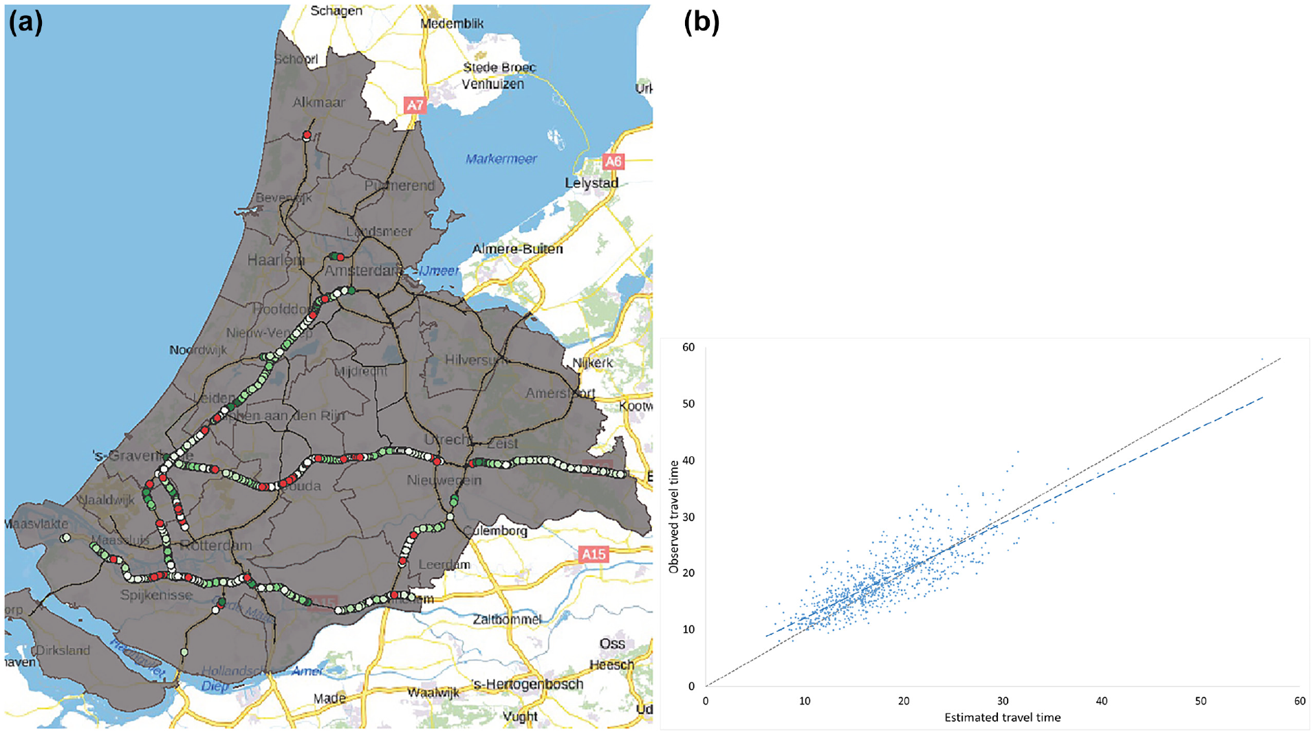
Traffic assignment formulation calibration: (a) mapped measurement points and (b) estimated versus observed congested travel time.
Base Year OD Matrices
The transport demand was estimated through incremental demand models, which means that the OD demands at the base year were required to estimate the demand at the next time step. Freight OD matrices were created based on the CSV data received from Statistics Netherlands (CBS). These data were processed and mapped uniformly from the NUTS2 or NUTS3 to the case study demand nodes. Freight flows to the whole Netherlands (both internal and external to the case study boundaries) were considered. Austria, Belgium, Denmark, Spain, France, Italy, Poland, and Sweden are included as international destinations and origins, accounting for the most tonnage transported from and to the Netherlands.
The road passenger OD matrix was estimated based on the available data from intensity measurement points. The data were retrieved from a national database for road transport ( 51 ) and mapped onto the road network to derive the intensities on the road segments, in addition to the inward and outward flow at each demand node. Using a Poisson distribution function, the number of trips for each distance category—within a 5 km range—was estimated. For the Poisson distribution, different average length trips in the range of 15 to 30 km were tested. This range was selected as CBS ( 56 ) reported an average trip length of 20 km in their annual report.
The Gauss–Seidel iteration method was then used to derive the OD matrix based on the total arrivals, departures, and the number of trips for each distance category. Afterwards, the estimated OD matrix was assigned to the road network. RMSE and the deviation between the estimated and the observed flows at each road link were inspected to minimize this deviation as much as possible. Through an iterative process, an estimated OD matrix was updated for specific pair of nodes, with high deviations in their adjacent road links. Comparing estimated OD matrices with different average trip lengths led to the conclusion that the average trip length of 25 km yields a more acceptable result. Thereafter, the final OD matrix was derived based on the 25 km average trip length. Figure 4 shows the assigned freight and passenger for the base year.
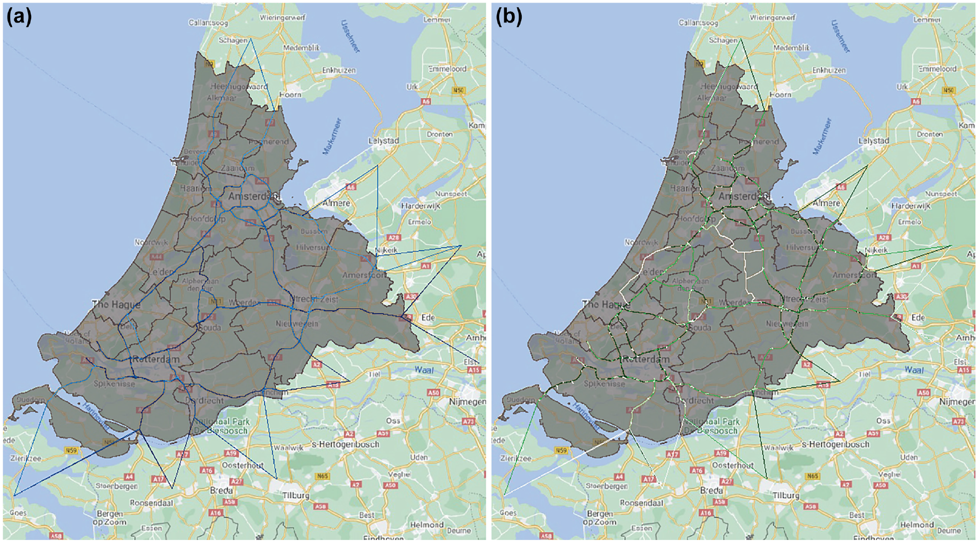
Base year flows: the darker the color, the higher the flow: (a) freight and (b) passenger.
Future Scenarios Adaptation
The four scenarios were adapted by quantifying inputs for the main determinants of transport demand as described in the Transport Demands Submodels section.
We adapted the scenarios by using the Shared Socio-economic Pathway (SSP) framework to define the direction and relative changes of the socio-economic variables. This framework provides a solid basis for coupling numeric values to demand determinants. The different futures of the SSP framework can be mapped onto the scenarios described here to adapt the scenarios based on the combination of climate policies and outcome projections, in addition to socio-economic conditions ( 57 , 58 ). Thus, the SSP framework enables adaptation of the scenarios consistent with their storyline, in which specific climate and socio-economic developments act as main drivers toward distinct futures. We then used the work of van Vuuren and Carter ( 59 )—which depicts future developments based on the SSP framework—to extract information about the direction and relative values of the demand determinant variables.
In a final step, scenarios developed by the Netherlands Environmental Assessment Agency (PBL-WLO scenarios) ( 60 ) were used to quantify context-related variables. The PBL-WLO scenarios envision two levels of high and low socio-economic and demographic growth, with values for changes in population, total and sectoral GDP, and the number of jobs for 2030 and 2050. These values are to a large extent consistent with the core scenario narratives, as well as the development directions of SSP variables. In the case of the latter, in-between development levels (e.g., moderate) for demand determinant variables are considered, where necessary. This is consistent with the storylines of the core scenarios and the development directions are derived from the SSP framework.
Table 6 shows the values of the demand determinants for each scenario. Change in energy efficiency and mix, in addition to the load capacity factor, indicates technological developments and diffusion within each scenario. Cubic spline interpolation was chosen to achieve a smooth and continuous curve for each variable in the simulation ( 61 ).
Emission, Energy, and Transport Demand Input Variables for Each Future Scenario
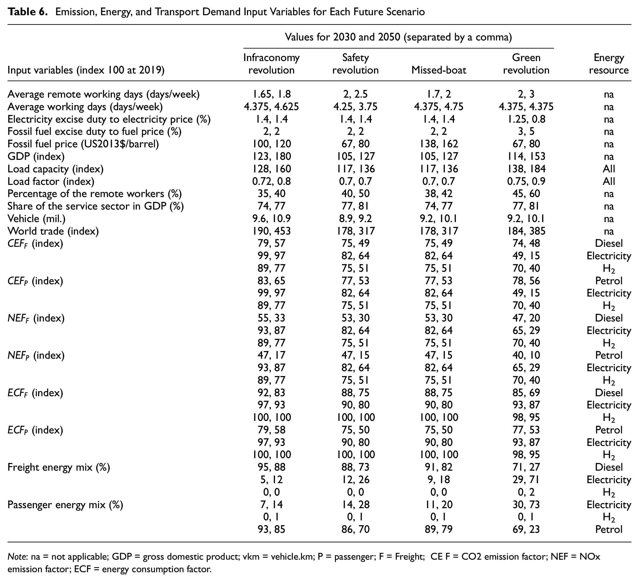
Note: na = not applicable; GDP = gross domestic product; vkm = vehicle.km; P = passenger; F = Freight; CE F = CO2 emission factor; NEF = NOx emission factor; ECF = energy consumption factor.
Consumer and Representative Energy Prices
In this analysis, each scenario is assumed to have a steady fuel and energy price trend. Considering all scenarios, the model includes different fuel and energy price levels and estimates the possible effects of these levels on road network demand. Fuel elasticity remains constant in this model, whereas the sensitivity of the transport demand to the fuel price depends on the fuel mix. For instance, in a future scenario where electricity has a bigger share in the fuel mix, the effect of the electricity price on transport demand is higher than the fossil fuel price. In this study, fuel price elasticity is considered because it is the only energy resource-related price–demand elasticity in the context of the Netherlands. At the same time, both electricity and fossil fuel have a major portion in the fuel mix among scenarios (minimum 96%). Their price changes were considered to trace their effects on transport demand. We defined the representative energy price, which is the weighted sum of electricity and fossil fuel consumer price (per kWh). Weights were derived based on the share of the energy resource in the mix in each simulation time step. Consumer electricity and fossil fuel prices for road users were based on the oil barrel prices, fossil fuel and electricity excise duty, and the share of the excise duty values in the energy resources’ consumer prices. Fossil fuel prices have a close correlation with oil barrel prices ( 62 , 63 ), therefore the changes of the oil barrel price were considered as a proxy for the fossil fuel price changes ( 60 ). Fuel excise duties are a main part of consumer fuel prices. Diesel and gasoline excise duty has been responsible for around two-thirds of the consumer price in the Netherlands in recent years ( 31 , 64 ). Electricity tariffs and excise duty were used to derive the consumer electricity price for road users ( 64 , 65 ). Excise duties are an important policy measure to reduce the road CO2 carbon footprint, which might develop differently under different future scenarios. Therefore, next to the changes in oil barrel price, excise duty changes were also considered. Among all scenarios, the changes were only applied in the Green Revolution scenario, because there is not an explicit political commitment to tackle emissions in the Infraconomy and Safety Revolution scenarios. In the Green Revolution scenario, a tax instrument aims to restrict the use of polluting energy resources and to further facilitate the transition to cleaner energy resources.
Emission and Energy Efficiency Factors
These factors change in time affected by financial and policy instruments, next to social norms, which facilitate technological advancement and diffusion ( 66 , 67 ). The base year factors ( 44 , 45 , 68 ) are projected according exploratory scenarios of the DLR ( 69 – 71 ). These projections within the context of the European Union fit the storylines of our scenarios. Our Green Revolution scenario sketches similar interventions to the Regulated Shift scenario, where regulations and investments aim to foster clean technology advancements. Our Infraconomy scenario is close to the Free Play scenario with a liberal market-economic logic. The advancements of the Reference scenario are used for both the Missed-Boat and Safety Revolution scenario, because of the moderate enhancements with regard to clean technologies. According to the cluster analysis of Neef et al. ( 22 ), Missed-Boat and Safety Revolution are likely to have similar technological advancement, which is mainly because of slow economic development. The emission factors include energy production and tailpipe emissions, which are estimated based on the plausible technological progression and diffusion and the governing policies within each scenario.
Fuel Mix
We considered fuel mix changes for passenger vehicles in each scenario but limited to Electricity, Diesel, Hydrogen, and Petrol based on Kugler et al. ( 72 ). To derive the fuel mix of Plug-in Hybrid Electric Vehicles (PHEV), a factor defining the share of fossil fuel in PHEV driving was assumed. This factor is 10%, 44%, 50%, and 65% for Green Revolution, Safety Revolution, Missed-Boat, and Infraconomy, in 2040 (time horizon of the Transport and the Environment projections). We distinguished the transition pace in the Safety Revolution scenario toward cleaner vehicles, as there are more societal consensus and acceptance to reduce emissions and enhance the quality of life. These assumptions were aligned with the scenarios’ narrative, which defined the dominance of fossil fuels in the transport sector. For fuel mix used in freight vehicles, we used passenger fuel mix with a 1% to 2% lag to account for possible inertia in companies.
Load Capacity and Factors
Load capacity projections were based on Groen et al. ( 73 ), which provides us with a context-relevant, yet lower-bound estimation. Green Revolution and Infraconomy have the highest increase as a result of transport efficiency. However, the former relates to the emission reduction target, whereas the latter has an economic motivation. Missed-Boat and Safety Revolution have the lowest development because of slower technological advancements as a result of slower economic growth. Logistics actions such as packaging, loading, and booking efficiency can increase the load factor, and thus increase transport efficiency ( 74 ). Similar reasoning holds for the exploratory load factor projections. The base year value is derived from CE Delft ( 45 ).
Socio-Economic Variables
GDP, population, and vehicle ownership changes are projected using the qualitative narratives of the core scenarios, SSP framework, and the values provided by the PBL-WLO scenarios ( 57 – 60 ). The municipality-level projections were used for population and jobs. The number of average working days was derived from the report of CBS ( 75 ) for the base year. This variable remains constant for the Green Revolution scenario, whereas it decreases for the Safety Revolution scenario, as people work less to enhance their quality of life. In the Infraconomy scenario, the average working days increase, to maximize economic gains. The same holds for the Missed-Boat scenario to compensate for a low income increase. The average remote working days were increased by 1.6 ( 34 ) in 2030 for all scenarios, to account for a possible long-term shift toward remote working in the COVID-19 aftermath. The differentiation among scenarios lies in the average remote working days and the percentage of remote workers and was aligned with the future pathways depicted by the scenarios. The Green Revolution scenario benefits from available infrastructures (e.g., reliable and secure ICT network) and social acceptance to allow for a high shift, whereas the Safety Revolution scenario misses such infrastructures despite the high social acceptance, which leads to a slower shift. In the Infraconomy scenario, in-person meetings are preferred. In the Missed-Boat scenario, the shift is limited because of the unavailability of the required infrastructures, as well as less social acceptance.
Globalization describes an important aspect of the scenarios and is the main determinant of international freight transport. The Netherlands Bureau for Economic Policy Analysis (CPB) introduced the world trade index as a proxy of globalization ( 32 ). In this paper, the world trade index was adopted for the Infraconomy, Green, and Safety Revolution scenarios based on the high and low PBL-WLO scenarios ( 60 ). For the Missed-Boat scenario, the world trade index projection considered the possible effects and extend of more global trade barriers. Global trade is closely related to global GDP growth, although the former develops with more volatility ( 76 ). For the Missed-Boat scenario, this means a slower increase in the world trade index. Higher tariffs and trade barriers translate into higher costs for consumers, and will not deliver the intended results argued by protectionist and populist states ( 77 ). Despite the possible rise of protectionism of major players, open plurilateral arrangements become popular, because such systems are beneficial for similarly structured economies (ESPAS 2019). Thus, global trade expands, although at a slower pace. The 2030 projected value for the low PBL-CPB scenario was considered for the Missed-Boat 2050 world trade index. The current effect of the COVID-19 pandemic was not considered in the world trade index projections, because of the long-term planning 30 years ahead.
Results
The road network transport demand during evening peak hours in 2050 is shown in Figure 5 and Supplemental Appendix A Figure 6 concerning the network delay and the pcu-e demand. Moreover, Supplemental Appendix A Figures 7 to 9 present the estimations for the performance indicators of the four scenarios in 2030 and 2050, the changes of transport, emission and energy consumption over time, and the emission and energy consumption per energy source.
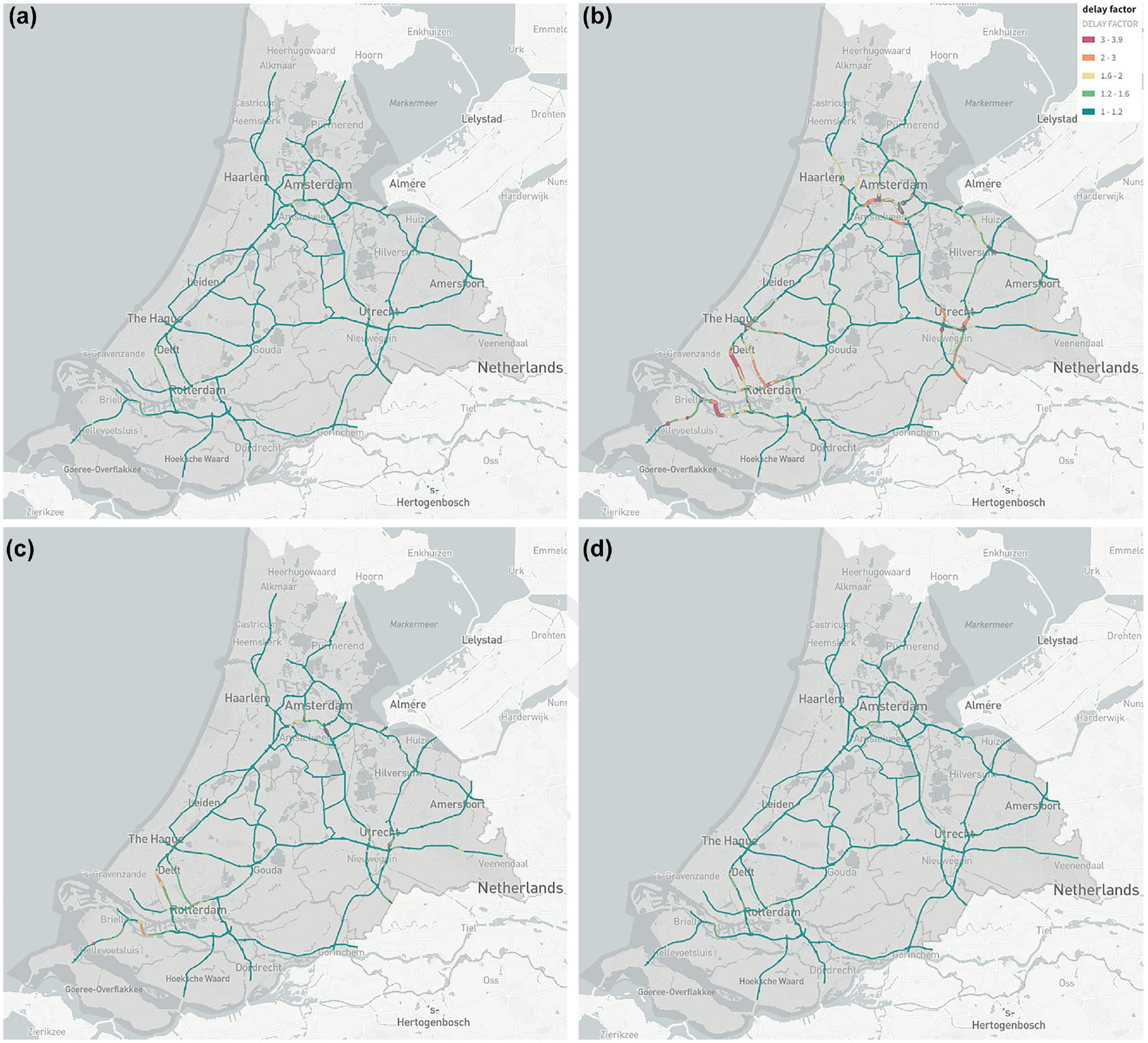
Delay factors in 2050: (a) Green revolution, (b) Infraconomy, (c) Missed-boat and (d) Safety revolution.
Scenarios’ Comparison
In Supplemental Appendix A Figure 8a, the freight demand volume in 2030 is the highest for Infraconomy followed by Green Revolution. Freight demands in the Missed-Boat and Safety Revolution scenarios are at similar levels and close to the Green Revolution. In 2050 (Supplemental Appendix A Figure 8b), the order stays the same but the gaps are bigger. Only the Missed-Boat and Safety Revolution scenarios stay close. In relation to the pcu-e freight transport, the Infraconomy scenario has the highest flow in 2039, while the Missed-Boat and Safety Revolution scenarios have the highest flow in 2050. Similar to the tonne freight demand, the Missed-Boat and Safety Revolution scenarios show similar performance levels. The passenger demand is the highest in the Infraconomy scenario for both 2030 and 2050. In 2030, the performance level in the Missed-Boat and Safety Revolution scenarios are again close and follow the Infraconomy and Green Revolution scenarios in pcu passenger demand. This changes in 2050, where the passenger demand in the Green and Safety Revolution scenarios are similar but lower than for the Infraconomy and Missed-Boat scenarios. Moreover, the gap between the Infraconomy scenarios and the other three scenarios grows significantly. Safety Revolution has the least demand.
CO2 emission and energy consumption have the highest values in the Infraconomy scenarios in 2030 and 2050, with an increasing gap between this scenario and the other three over the simulation period. In 2030 the performance differences are small among the Green Revolution, Safety Revolution, and Missed-Boat scenarios but grow In 2050. NOx emission levels are close for all four scenarios in 2030, especially for the Infraconomy, Missed-Boat, and Safety Revolution scenarios. In 2050, the NOx emission difference between Green Revolution and three other scenarios grows, whereas the other three show similar performance levels. This closeness can be explained by an expected response to the probable stricter regulations and controls for NOx emission ( 70 , 78 ).
Green Revolution
Freight demand (Supplemental Appendix A Figure 7a) increases continuously until 2050. This can be explained by the relatively high GDP and world trade increase. The electricity price decrease slows down the representative energy price increase and limits its negative effect on freight demand. From 2044 onwards the combined effects of the electric vehicle increase and electricity price decrease diminish the representative energy price and, thus, have a positive effect on freight demand. On the other hand, the increase in the share of service-sector GDP slows down the tonne freight demand increase. The passenger unit car equivalent (pcu-e, Supplemental Appendix A Figure 7c) of freight demand, however, decreases. This can be explained by the relatively high increase in the fleet load capacity and load factor, which reflects technological and operational developments in improving transport efficiency. This decrease slows down as the tonne cargo demand increases.
Passenger demand (Supplemental Appendix A Figure 7b) first increases slightly until 2028 and then drops 15% below the base year value in 2050. The increase can be explained by a relatively high increase in GDP and the number of jobs, in addition to a moderate increase in the number of vehicles, and finally, a slight increase in the population until 2030. Continuous and relatively high increase in the remote working-related variables, the representative energy price increase and the population decrease from 2030 onward negatively affect the passenger demand. These variables dampen the passenger demand increase until 2044 and thereafter result in a demand decrease. After 2044 the representative price drops push the demand upwards. This passenger demand trend suggests that the negatively affecting variables have a higher impact on passenger demand compared with the variables that increase the demand (e.g., GDP).
Emission and energy consumption (Supplemental Appendix A Figure 7, d–f) decrease prominently (between 60% and 80%) in this scenario as the result of fast and continuous technological advancements and diffusion, a major behavioral shift in relation to remote working, and the removal of fossil fuels from the fuel mix. It is noticeable that the effect of vehicle efficiency, cleaner energy production, change in fuel mix toward more environmentally friendly energy sources, and decrease in freight pcu-e, counterbalanced the slight decrease in pcu passenger demand until 2028. This results in a continuous and steep decrease in emission and energy consumption. In fact, the major shift toward cleaner energy sources in transport decouples emissions from pcu-e transport. Emission and efficiency enhancements in energy production result in an emission decrease by reducing the well-to-tank (WTT) emission.
Infraconomy
The results provide us with insights into the freight and passenger transport demand, energy consumption, and emissions for a scenario in which economic development is the key force in shaping the future. Tonne freight demand increases perpetually, which can be explained by the high increase in GDP and world trade. The share of service-sector GDP grows more slowly in this scenario, which limits its impact on decreasing the freight demand. Similarly, a relatively high increase in fossil fuel price does change the effect on freight demand. The electricity price stays constant. Therefore, only a shift to electric vehicles affects the representative energy price, which slightly balances out the sharp fossil fuel increase. Freight pcu-e, however, decreases continuously. This suggests that the combined effect of fleet load capacity and load factor is effective in decreasing the freight pcu-e. However, such a decreasing effect slows down over time because of a sharp freight volume demand.
Passenger demand increases continuously, which can be clarified by the fast increase in GDP, the number of jobs, population, and vehicles. Fossil fuel prices increase noticeably: around twice the base year value in 2050. Although this negatively affects passenger demand, it does not lead to a demand trend change. One reason is the dominant effect of the positively affecting variables. Moreover, the shift to electrical energy balances out the fossil fuel price increase. That slows down the representative energy price increase, and thus limited its negative effect on demand.
Energy consumption, CO2, and NOx emissions decrease continuously, which can be mainly attributed to emission and energy efficiency enhancements in fossil-fueled vehicles. Efficiency progressions are the strongest among all scenarios, as they address the main fleet type and sustain their competitive advantages compared with other fleet types that are not incentivized. However, these efficiency gains reach their limit sooner than a switch to cleaner vehicle types. Moreover, energy production depends mainly on fossil fuels, which limits the WTT emission reductions compared with alternative energy resources. The efficiency increase saturation and a modest shift to cleaner energy resources, together with a continuous increase in passenger demand reduces the rate of emission and energy consumption. Contrary to CO2 and energy consumption, NOx emission drops to a level close to that of other scenarios and stabilizes for the last 10 years.
Missed-Boat
The tonne freight demand slightly decreases for the first 7 years and then increases to 10% above its base year value in 2050. The reason behind the initial demand decrease seems to be the noticeable effect of the high fossil fuel price in relation to a slow increase in the service-sector GDP. These developments balance out the demand increase stemming from the (slow) GDP and world trade increase. It should be noted that the shift toward electric vehicles only dampens the effect of the fossil fuel price increase on the freight volume demand through the representative energy price. This limited influence can be further explained by the lack of incentives to encourage a transition toward cleaner resources. A steeper increase in world trade after 2030 compared with the first 10 years positively affects freight demand. Moreover, GDP grows more in the last 20 years, which also plays a role in changing the trend and increasing the demand. Load capacity develops in a way that the freight pcu-e decreases, despite the continuous tonne freight increase. The pcu-e freight flow stays almost constant in the last 12 years and becomes 26% lower than the base year in 2050.
Passenger demand decreases in the first 6 years, then increases to a value in 2050 around 5% higher than the base year value. The combined effect of high fuel price (highest among all scenarios), average remote working, and percentage of remote workers seem to account for the decrease in passenger demand in the first 6 years, despite the increase in average working days, the number of jobs, vehicles, GDP, and population. These variables become dominant over time and increase passenger demand. It is important to stress the relatively high elasticity of passenger demand to the number of commuting jobs—affected by the remote working variables and average working days—which plays an important role in increasing passenger demand. Furthermore, the fossil fuel price increases more slowly in the last 20 years. The effect of fossil fuel prices on the demand further slows down with a moderate shift toward electric vehicles. In addition, the negative effect of the energy price on passenger demand lessens after 2030.
In the Missed-Boat scenario emission and energy consumption decrease continuously. This suggests relatively low levels of freight and passenger demand on the one hand and technological advancements and a shift toward cleaner energy sources on the other hand. The decrease slows down because of the change in transport demand, the saturation of emissions, and the energy efficiency of vehicles and energy production facilities, which still mainly depend on fossil fuels. Moreover, the increase in pcu-e freight and passenger demand leads to higher emissions.
Safety Revolution
Freight demand stays almost constant for the first 12 years and then increases to 10% above its base year value in 2050. A faster GDP and world trade after 2030 result in a steeper freight demand increase. The fossil fuel price increase is relatively slow in this scenario. Furthermore, a moderate shift toward electricity in the transport fuel mix dampens the effect of the fossil fuel price on freight demand. Moreover, this scenario has a relatively high transition toward a knowledge- and service-based economy, which decreases the freight demand. Similar to the Missed-Boat scenario, the pcu-e freight demand stays constant in the last 12 years and ends up 25% lower than the base year value.
In this scenario, passenger demand stays quite stable for the first 6 years and then decreases. Although the GDP, number of jobs, and vehicle ownership positively affect demand, the remote working variables and the representative energy price seem to counterbalance the demand increase. Here, population and number of jobs—both increase in the first 10 years—have the most significant impact because of their relatively high elasticity values. Their decrease from 2030 onward plays an important role in the change from demand stability to demand decrease.
Emission and energy consumption decrease continuously in this scenario. This can be attributed to the moderate technological advancements in the emission and energy efficiency of vehicles and energy production facilities. The latter affects WTT emissions and the former influences tank-to-wheel emissions. Additionally, changes in the vehicle fuel mix result in the use of more clean energy resources, and thus, reduced emissions. As mentioned earlier, NOx emission drops noticeably, yet to a level close to Infraconomy and Missed-Boat scenarios. That happens, despite the different fuel mixes, and emission and energy consumption factors of these scenarios.
High-Resolution Validation
The presented results are compared with the long-term forecast of the Dutch National Model System (LMS). The Infraconomy scenario is compared with the High PBL-WLO scenario (introduced in the Future Scenarios Adaptation section) because the shared socio-economic variables of the proposed model and the LMS match for these two scenarios. Moreover, the Infraconomy scenario depicts a future with the highest transport demand increase among all scenarios, which can be compared with the High PBL-WLO. Wijlhuizen et al. ( 79 ) published an updated LMS simulation run for the main road network on the national level, which is used to compare the estimated freight tkm and passenger vkm demand. The freight tonne and passenger vkm forecasts of the PBL-CPB ( 80 ) for all roads on the national and the Randstad region (the northwestern part of the Netherlands) is also used for the validation of freight volume and passenger demand. The case study region in this paper matches the geographical boundaries of Randstad to a great extent. Most of the freight demand is generated in the case study region where the main highways and the two biggest national ports are located. The regional difference in passenger demand is bigger than the national-level comparison. For the demand estimation in the Randstad the LMS includes all roads, whereas for the national level only main roads are considered. The differences between the presented model and the LSM are within a 5% range (Table 9). The presented model tends to overestimate freight tonne and tkm while underestimating passenger vkm demand in 2030 and 2050 on the regional and national levels, respectively.
Discussion
Understanding the Demand and Performance Indicators Under Different Futures
In this sub-section, we discuss the implications of the four future scenarios on transport demand, and environmental and road network performance indicators.
Road Transport Demand
Freight Demand
Freight volume demand increases in all scenarios, but with different rates. The most influencing variable is the share of service-sector GDP in the total GDP (GS), which negatively affects the demand and increases in all scenarios. In the Green and Safety Revolution scenarios this variable increases the highest and dampens freight demand. However, it has no trend-changing effect in all scenarios. The representative energy price increased in all scenarios except for the last 6 years of the Green Revolution. This price increase could barely affect the increasing trend of demand. In the Green Revolution where the electricity tax decreases with an increase in the share of electric vehicles, the representative energy price decreases. This pushes slightly the demand higher. High freight demand in the Infraconomy scenario matches the expected scenario image, where economic growth is coupled strongly with global trade, and high GDP development fosters domestic freight haulage. In the Green Revolution scenario, world trade and GDP develops slower than in the Infraconomy scenario, which results in milder freight growth. This partly reflects the shift toward a more local, knowledge- and service-based economy. Despite the shift, freight demand is expected to grow by around 25% by 2050. The Missed-Boat and Safety Revolution scenarios show close freight demand because of their similar GDP and world trade changes. This is also validated by the cluster analysis of the Delphi study for the scenario development ( 22 ). Different energy prices and GS have minor effects on differentiating between the aforementioned two scenarios. It is noticeable that although the GS is higher in the Safety Revolution scenario, the freight is higher in comparison with the Missed-Boat scenario. This can be explained by a higher representative price as a result of the fossil fuel price change and a higher share of fossil fuel-driven vehicles.
Load capacity and load factor change directly affect the pcu-e freight demand of road infrastructure ( 74 ). The load factor only increased in the Green Revolution and Infraconomy scenarios. In the former, infrastructure efficiency enhancements are explicitly envisioned and invested in. In the latter, it is a product of technological advancement and an economic-oriented mindset. Depending on the freight volume increase and the capacity of the road network, the reduction of road traffic through more efficient transport can be evaluated. In the Green Revolution scenario efficiency enhancements decrease the number of trucks on the road (around 52%), whereas the volume demand is increasing. In the Infraconomy scenario, the pcu-e number is reduced by around 26%.
Passenger Demand
Changes in the number of commuting jobs per municipality, vehicle ownership, GDP, municipality population, and representative fuel price affect passenger demand. Only the latter affects the demand negatively. Looking at the projections, the Infraconomy and Safety Revolution scenarios are expected to sustain their increasing and decreasing trends, whereas in the Green Revolution and Missed-Boat scenarios demand shifts from increase to decrease and vice versa are estimated. It seems that the distinct differences in remote working behavior and vehicle ownership lead to these sustained, yet different trends. In the Infraconomy scenario, the highest passenger demand is estimated. That matches the future scenario image where users are prone to commute more and use the road infrastructure more intensely, with high numbers of available and affordable vehicles. On the contrary, a societal mindset toward enhancing safety and wellbeing reduces road commuting, resulting in a constant decrease in passenger demand.
In the Green Revolution and Missed-Boat scenarios, it is more important to consider the combined effects of all variables. Despite the highest level and rate of remote working, the Green Revolution scenario faces a higher passenger demand than the Missed-Boat scenario. In the Missed-Boat scenario, the combined effects of remote working and representative energy price lead to decreasing demand for a period of 6 years. Thereafter, the effect of population and GDP growth takes off and pushes the demand upwards. In contrast, the shift toward the reduction of work-related commuting in the Green Revolution scenario could only slow down the demand increase in the initial years. Here, incentivizing the shift toward cleaner energy sources by offering tax exemptions leads to rebound effects. In the Green Revolution scenario, tax exemptions and a fast transition to cleaner vehicles lead to cheaper energy prices. That affects the representative energy price by equalizing the positive effect of the heavily taxed fossil fuels. This phenomenon continues to the point where the representative energy price starts decreasing and the passenger demand increases. In these scenarios, we could clearly see the effects of income—through GDP—and energy prices on passenger demand in the short term, which can counterbalance demand management efforts. In 2050, however, the Missed-Boat scenario ends up around 5% above its base year value, whereas the Green Revolution scenario has a 15% passenger demand decrease. In the former scenario, the road performance is expected to worsen (Supplemental Appendix A Figure 6, a–d).
It is worth mentioning the distinct futures that the Infraconomy and Missed-Boat scenarios depict with the same population, where the former has around 35% more passenger demand. It clearly shows the strong combined effect of remote working and the number of jobs, the influence of income increase, and the interaction of fossil fuel prices and the shift toward cleaner energy sources on passenger demand. These variables have a more noticeable difference between the Infraconomy and Missed-Boat scenarios. From a road performance point of view, the Missed-Boat scenario appears preferable. However, in this scenario, the environmental, socio-economic, and political situation is more fragmented, unstable, and weaker, which directly affects social wellbeing and prosperity.
Similarly, the Green and Safety Revolution scenarios represent futures with the same population but the difference in demand is smaller. More jobs in the Green Revolution scenario make the remote working shift less effective, and income increases and vehicle ownership cause a demand increase for a certain period of time. Again, the effect of income increase on the demand is the most prevailing. The fossil fuel price difference between the Green and Safety Revolution scenarios also contributes to the demand difference, but to a lesser degree. This weaker effect can be explained by a low elasticity and the relatively high adoption of electric vehicles in the Green Revolution scenario. From the road network perspective, in the Green Revolution scenario, there is more capacity to enhance and maintain the existing network and support infrastructures for emerging vehicle technologies. We discuss these issues in the next sub-section.
Road Infrastructure Performance
Network Performance
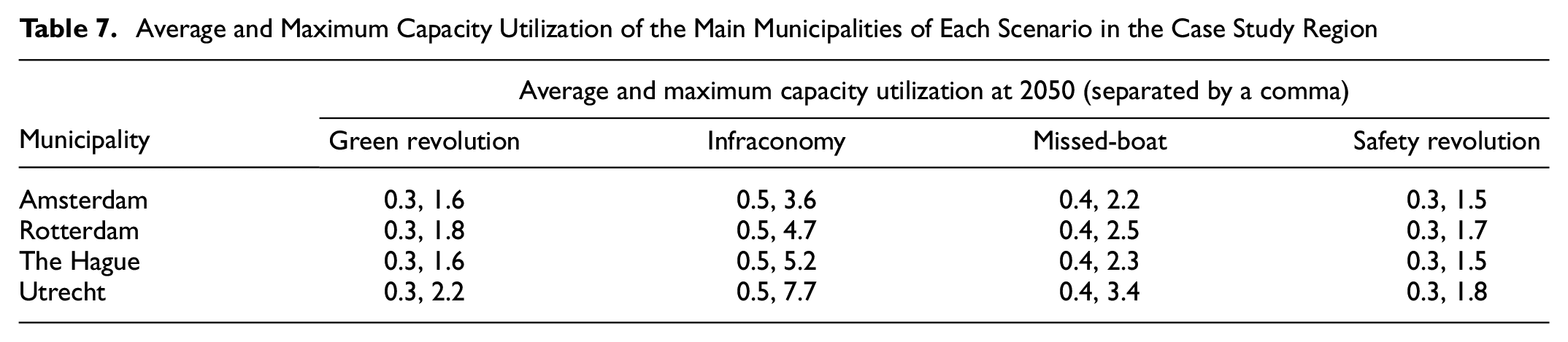
Table 7 shows the average and the highest capacity utilization ratios for four major industrial and urban municipalities in the case study region in 2050. The ratios are the highest in the Infraconomy scenario, followed by the Missed-Boat, Green, and Safety Revolution scenarios. Figure 5 shows the network-wide delay factors in the year 2050 for the four scenarios. Capacity utilization and delay factor follow the network-wide transport demand development (Supplemental Appendix A Figure 6, a–d ). As pcu-e freight transport is negligible compared with passenger demand (Supplemental Appendix A Figure 7, c and b ), road network performance is largely influenced by passenger demand. If the road network stays at the current capacity level, it will show noticeable capacity problems and delays in the Infraconomy scenario. In the Green and Safety Revolution scenarios, the road network is likely to have the least bottlenecks. In the Missed-Boat scenario road network performance probably faces more impediments, firstly because of more utilized and congested roads, and secondly because of the increasing trend of the pcu-e after 2030.
Average and Maximum Capacity Utilization of the Main Municipalities of Each Scenario in the Case Study Region
Environmental Performance
In Supplemental Appendix A, Figure 9, a to c, indicate that CO2 emission and energy consumption show a similar trend. In 2030, in the Infraconomy scenario, they have the highest values, whereas in the other scenarios the performance levels are closer to each other (especially in the Missed-Boat and Safety Revolution scenarios). This can be explained by the high pcu-e transport demand in the Infraconomy scenario and the slow transition toward cleaner energy resources. Although the efficiency of fossil fuel-driven vehicles quickly develops in this scenario, it is not sufficient to significantly decrease emissions and energy consumption. Lower pcu-e transport demand in the Green Revolution, Missed-Boat, and Safety Revolution scenarios also leads to less emission and energy consumption. In 2030, the Missed-Boat scenario has the highest level of emission and energy consumption among these three scenarios, and the Green Revolution scenario has the lowest. This suggests that both transition pace and technological advancement are influential enough to decrease emission and energy consumption for a scenario with a high pcu-e transport demand. NOx emission in 2030 is noticeably reduced for all scenarios as a result of stricter regulations and control. Most of the emissions come from diesel and energy production facilities. In 2050, the Green Revolution scenario is the least polluted future with WTT emissions by electric vehicles as shown in Supplemental Appendix A Figure 9b. Electricity production causes these emissions and has almost a 60% share in NOx emission in this scenario. The NOx decreasing trend slows down and stabilizes for all other scenarios. The reason is the extent to which fossil fuels are utilized in vehicles and energy production facilities and the efficiency advancements for these fuels that reach their limits sooner than cleaner energy resources.
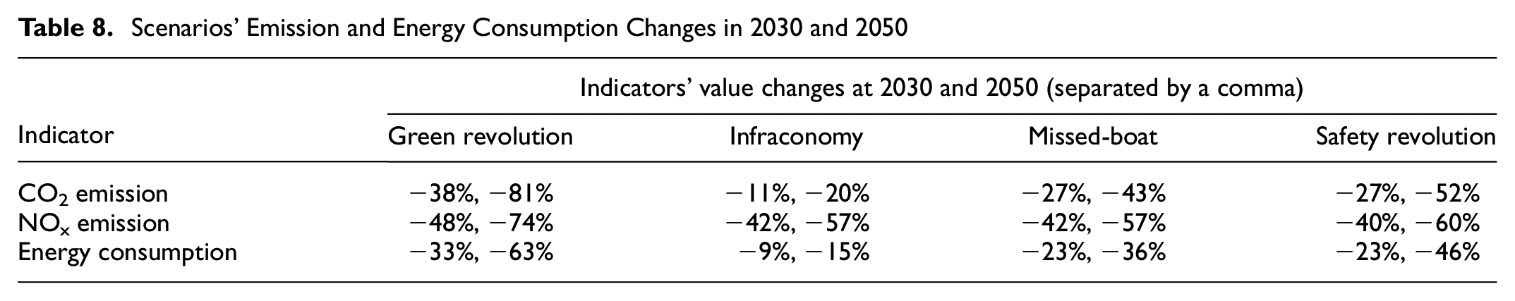
Table 8 presents the emission and energy consumption reductions per scenario in 2050. The Infraconomy scenario depicts a future in which technological advancement and transition to cleaner energy resources have a modest effect on emission and energy consumption to outweigh the environmental impact of pcu-e transport demand. It is the consequence of a slow transition to cleaner energy resources and technological advancement in transport and energy production. In this scenario the decreasing rate slows down and will turn into an increasing trend beyond 2050 in the light of ever-growing and not actively controlled pcu-e transport. The Missed-Boat scenario has the second-highest emission and energy consumption level. Climate mitigation and adaptation efforts reduce this level more than in the Infraconomy scenario. However, over time and because of the weak economic growth and the fragmented political atmosphere, the possibilities for imposing effective policies, advancing energy and vehicle efficiency, creating required infrastructure for cleaner energy production, and remote working will diminish. Emission and energy consumption then may follow an increasing trend beyond the year 2050. In the Safety Revolution scenario, the lower pcu-e demand as a consequence of fewer work-related commutes has the most significant influence on the relatively low levels of emission and energy consumption (10%–25% lower than for the Missed-Boat scenario in 2050). The reduction of emission and energy consumption by 80% in the Green Revolution scenario is expected to continue as a result of further decrease in pcu-e transport demand, progressions in energy transition, and technological advancements. Compared with the Safety Revolution scenario, in the Green Revolution scenario climate change mitigation and adaptation efforts are more effective combined with a faster economic growth.
Scenarios’ Emission and Energy Consumption Changes in 2030 and 2050
Results’ Comparison With LMS Model
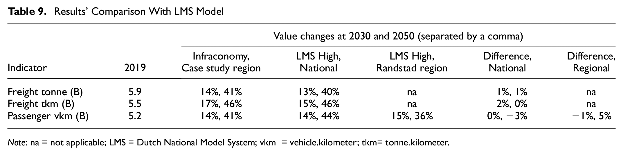
Note: na = not applicable; LMS = Dutch National Model System; vkm = vehicle.kilometer; tkm= tonne.kilometer.
The European Union has set an updated Paris Agreement target to reduce emission at least 55% (including LULUCF sector) by 2030 ( 81 ), while aiming for a net-zero greenhouse gas emission by 2050 (compared with 1990), which corresponds to a maximum global temperature increase of 1.5° Celsius. At the same time, the EU considers a temperature increase between 1.5° and 2° Celsius an acceptable range for which it targets ( 82 , 83 ). We assume the same targets being uniformly transformed for emission and energy consumption arising from road transport and evaluate the compliance with these targets for both CO2 and NOx emissions. Given that the overall greenhouse emission decreased 10.7% in 2019 compared with 1990 ( 78 ), none of the scenarios reach the target in decreasing CO2 emissions in 2030. As presented in Table 8, the Green Revolution scenario is the closest with a 38% and 48% emission reduction for CO2 and NOx, respectively. NOx emission is reduced significantly in all scenarios by 2030, but only the Green Revolution and Missed-Boat scenarios meet the reduction target. Until 2030, by assuming the same emission reduction share for road transport as for the total reduction, we can expect the Green Revolution, Missed-Boat, and Safety Revolution scenarios to be in line with keeping the temperature increase between 1.5°C and 2°C. The Infraconomy scenario results in a temperature increase between 2°C and 3°C ( 84 ). Emission neutrality is not expected to be achieved in any scenario in 2050, even in the Green Revolution scenario with directed and intensive commitments and measures to reach climate and energy targets. It can be expected that only the Green Revolution scenario can stay within the 1.5–2°C temperature increase, whereas the Safety Revolution, Missed-Boat, and Infraconomy scenarios can be expected to end up with a 2–3°C increase, respectively, (ordered from low temperature to high) ( 84 ).
Possible Infrastructure Investments Under Different Futures
Infrastructure investments that aim to address the socio-economic developments mainly consist of extension and maintenance to enhance or keep infrastructure performance at a desired level ( 85 ). In this section, we elaborate on possible investments for the investigated road network based on the estimated demand and performance and discuss major investment shifts between the four scenarios. The main assumption is that social and governance attitudes and priorities remain consistent with their initial states for each scenario.
Green Revolution
In the Green Revolution scenario, road infrastructure performs without major obstructions in 2050 (Figure 5a). The decreasing transport demand reduces the load on the road network even beyond 2050. That can keep road infrastructure expansions limited to a few roads around the four major industrial and urban areas in the case study region (Amsterdam, Rotterdam, The Hague, and Utrecht). Alternatively, bottlenecks are accepted until the decreasing demand comes into effect and reduces the criticality of the congested roads.
The rebound effect of vehicle ownership might create congestion, because a cleaner fleet and their supporting infrastructure become available, affordable, and allow longer-range travels. An environmentally friendly image of road transport can lead to more trips ( 86 , 87 ). This can be more prevalent in societies that are sensitive to the environmental consequences of transport. It should be noted that we treat vehicle ownership as an input variable and consider such a rebound effect by assuming a relatively higher input value. It is expected that (semi and fully) autonomous vehicles are rolled out at the highest level in this scenario, which has both reinforcing and balancing effects on road congestion. It is expected that such a technological trend increases congestion in urban areas while decreasing the congestion on highways ( 88 , 89 ). The congestion increase can be mainly attributed to the possible shifts from other modalities because of the possible increase in travel convenience and better accessibility within the urban regions to be provided by the autonomous vehicles, whereas the congestion decrease can arise from greater transport efficiency and enhanced driving behavior, which leads to higher road capacities. Overall, in this scenario, there should be preparedness to control and accommodate possible demand rebound effects. A more extensive investigation is needed to better quantify these effects on road demand and congestion that affect the expansion investment decision-making.
In the Green Revolution scenario, investments in road infrastructure shift toward accommodating the need for renewable energy generation and utilization and charging infrastructures, for example, fast charging stations ( 90 ). Maintenance investment needs that arise from infrastructure utilization are expected to decline. Moreover, such investments can incorporate a wider range of functional improvements, for instance, to enable charging while driving. Transport emission decreases by shifting toward cleaner technologies, but there is a risk of emission increase related to extraction and production processes, as well as adverse environmental consequences of managing the end-of-life elements. Although such risks can be higher in the Green Revolution scenario as a result of its fast and extensive transition, this scenario has high capacity, capital, and technological resources to manage them. The higher-level policy can affect the decisions of road infrastructure agencies, for instance in increasing the accessibility of recycling facilities and the related logistics needs.
Infraconomy
Figure 5b shows that in the Infraconomy scenario the road network is heavily congested, both in the order of magnitude and spatial extent. Therefore, infrastructure expansion is likely to be necessary, especially when such a strategy is aligned with the dominant mindset of this scenario. Investments are likely to take place around the major four urban areas in the region and along the major south–north and east–west freight routes. Because of significant capacity utilization, the road network deteriorates faster and more severely. This increases the probability of maintenance investment needs. Additionally, because of a continuous increase in transport demand, ensuring and enhancing safety and noise reduction can become critical and need to be prioritized. Countermeasures to enhance safety can include modifying the layout of physical infrastructure or the implementation of intelligent ICT solutions in both vehicles and infrastructure ( 91 , 92 ). Noise and pollution are expected to increase sharply, which may limit the infrastructure expansion strategy.
Missed-Boat
As Figure 5c shows, in the Missed-Boat scenario road congestion is limited to a few connection roads around the four major industrial and urban areas in 2050. However, transport demand increases, which leads to further congestion and probably worsens road performance. Consequently, road network capacity expansion may become necessary in this scenario to accommodate future demand. That exposes the Missed-Boat scenario to the risks arising from accidents, noise, and pollution, as a result of increasing transport demand. Moreover, in the long run (for example, end of this century) and compared with the Green Revolution scenario, emission levels may increase the occurrence and intensity of climate-related extreme events. Although the consequences of the issues mentioned above are probably less than in the Infraconomy scenario, it is also possible that in the Missed-Boat scenario strategies are required to ensure continuous and desirable road network functionality. This scenario is likely to remain limited in providing the required measures because of the unstable and fragmented policy sphere. In addition, weak economic growth may limit the financial and governance capacities to tackle the challenges. This can lead to a lock-in situation for the road network performance in light of a long-term transport demand increase.
Safety Revolution
In this scenario, transport demand decreases continuously, which reduces the probability of necessary capacity expansion. After the Green Revolution scenario, this scenario has the fastest and more extensive energy transition. Thus, the rebound effects of alternative vehicle types are likely to increase transport demand, but such an increase is lower than in the Green Revolution scenario. Consequently, accidents, noise, and pollution impacts diminish. Therefore, tackling these issues probably becomes less urgent compared with the Infraconomy and Missed-Boat scenarios. Population shrinkage in 2050 decreases the need for infrastructure capacity expansion and creates more space. This allows infrastructure development while maintaining livability standards. As mentioned previously, the Safety Revolution scenario is likely to face similar climate-related long-term consequences as the Missed-Boat scenario, while having a comparable financial capacity. However, compared with the Missed-Boat scenario, the wellbeing-directed policy and mindset, more available space, and low population, can potentially better facilitate countermeasures. However, these measures are capital-intensive and probably push for a shift in investment prioritization. For instance, maintaining and expanding the road network to account for the energy transition may become limited. It should be noted that the reduced maintenance investment needs resulting from a reduction in infrastructure utilization can provide the necessary investments with extra resources.
Conclusion
The proposed model in this paper enables us to evaluate the effects of distinct behavioral, socio-economic, policy, and technological changes on road transport performances, and addresses the related uncertainties. It aims to support infrastructure investment decisions primarily by tracing the performance changes under different future scenarios, presenting a set of performance indicators, and attaching relevant temporal and spatial information. This model thus intends to provide insights on investment needs based on estimating infrastructure demand and performance, which include maintenance, possible capacity extension needs, and required interventions to respond to emerging transport technologies and behaviors. Moreover, possible investment shifts within each future scenario and their possible consequences for road performance are presented. This research facilitates detecting the required investments on different levels, from a whole case study region to finer regional levels. Thus, this model can encourage decision-making across different managerial and governance levels in charge of road infrastructure.
Next to infrastructure investment decisions, the proposed scenario-based model can assist in policy decision-making that gives shape to certain future pathways. The effects of policies that aim to manage transport demand and facilitate behavioral and technological changes toward production and use of cleaner energy sources on the performance of infrastructure can be traced. This paper considered economic, demand management, and pricing measures, which affect the extent of remote working, shift in the transport fuel mix, and efficiencies in emission and energy consumption as a result of technological progression and diffusion in energy and automotive production sectors. Change in the economic structure toward the service- and knowledge-based economy reduces freight volume demand. However, on the international level, world trade has a more dominant effect, which makes the effect of such a transition dependent on the extent to which it can be reflected on a global scale. It should be noted that the mentioned economic shift can be partly considered by the presented model. To better understand this phenomenon, which has a strong presence in the Green Revolution scenario, more in-depth analysis is needed. Furthermore, the demand management strategy has a pronounced effect on passenger demand, where Infraconomy has a sharp increase and Missed-Boat contains the increase, and on the contrary Green and Safety Revolution experience a decrease in demand. The effect of demand management can also be seen in emissions and energy consumption. We can expect better performance where passenger demand is better contained. Energy transition policy measures further decrease emissions and energy consumption. On the one hand, such policies incentivize a faster and more extensive transport fuel mix transition. On the other hand, a shift in cleaner energy production technologies and efficiency enhancements in vehicles reduce emissions and energy consumption.
It should be noted that the mentioned policies, especially those targeting energy transition, require coordinated, beyond-boundary efforts, to ensure effective and timely responses. On the one hand, emission consequences (e.g., extreme climate events) are not bound to a certain geographic boundary; on the other hand, structural shifts (e.g., in the automotive industry) involve multiple actors distributed across the globe. Moreover, sustaining the long-term targets and required responses is of importance. Meeting 2030 emission goals—as is estimated for Missed-Boat and Safety Revolution—does not obviously guarantee meeting the longer-term targets in 2050 and beyond that to contain the temperature increase. It is worth mentioning that policies affecting performance and environmental performances go beyond the above-mentioned ones, for instance, carbon pricing and measures explicitly influencing vehicle ownership and usage such as taxation and road pricing. It is possible to indirectly include some of them in the presented model, by reflecting the carbon pricing in the fuel price or choosing consistent input value for vehicle ownership; however, a more dedicated quantitative analysis can further enrich the proposed model’s insights.
Elasticity values remain constant and are similar for each scenario, whereas in a specific future and after a certain point of time, some of the values can affect demand differently, for example, the effect of fuel price. Deriving such values can be challenging. The data and models from which such elasticity values can be derived and describe distinct future pathways are scarce. Moreover, it is expected that they are subject to high uncertainties, as they probably reflect stated choices in the future. Furthermore, input variables are another source of uncertainties within each scenario, which can be addressed by assuming bandwidth (consistent with the scenario narrative) around dominant variables. However, uncertainties should be accepted to a certain degree as imposing uncertainties shift to selecting the ranges in which variables change.
Future studies could look into the behavioral and technological changes in response to policy measures, the uptake of certain technologies, and the shift in social norms. For instance, the proposed model could be extended to include the possible induced demand arising from the uptake of cleaner vehicles. Another potential extension relates to the effects of fossil fuel taxation on users’ behavior and on the adaptation strategies and outcomes of the involved industries. This would better account for the dynamic pathways of future energy demand, travel behavior, and technological advancement and diffusion. Moreover, it is assumed that the scenarios remain constant in the major elements of their storylines; for instance, economic developments sustain their trend (whether slow or rapid). The anticipatory power of the model could be further increased by including (one or more) scenario(s) that contain fluctuations or shifts in certain trends (e.g., from climate-driven to economic-driven). Further developments could cover demand determinants beyond the socio-economic variables, such as travel time. This would reflect constraints imposed by infrastructure capacity. We argue that such constraints together with planned or expected capacity extensions can dynamically address infrastructure capacity changes in demand estimation. Investments in other transport networks can affect road transport demand and performance; for instance, an increase in train frequency and capacity can lead to higher perceived travel convenience, and thus can attract more passengers. That, in return, can decrease road network congestion and reduce the need to introduce capacity extension investments to the road network. Consequently, considering investments planned in other transport networks can give more insight into the transport demand and performance dynamics and can reduce uncertainties in the demand and performance development trajectories. The presented model can inform decision-makers in the investment identification phase to detect regions around which interventions in transport networks can enhance road network performance, therefore improving the flow of individuals and goods. Planned (or expected) investments under different future scenarios can be evaluated to inform decision-making. The effect of infrastructure provision on the demand should be considered as well, to achieve a more realistic demand and performance estimation.
Supplemental Material
sj-pdf-1-trr-10.1177_03611981221143377 – Supplemental material for Scenario-Based Strategic Modeling of Road Transport Demand and Performance
Supplemental material, sj-pdf-1-trr-10.1177_03611981221143377 for Scenario-Based Strategic Modeling of Road Transport Demand and Performance by Sahand Asgarpour, Andreas Hartmann, Konstantinos Gkiotsalitis and Robin Neef in Transportation Research Record
Footnotes
Acknowledgements
The authors would like to thank the experts of the infrastructure agencies involved in the knowledge institute NGInfra for their contributions to the research. Special thanks to Giel Jurgens, Jenne van der Velde, and Dr Mark de Bruijne from the NGInfra Accessibility Theme-center (Themacenter Beschikbaarheid) for facilitating the knowledge and data exchange with NGInfra experts. The authors also thank the present and former MOVICI team, especially Andrés Morales, Barış Demirdelen, Eelco Naarding, Martijn Stroeven, and Pelle Koster for contributing to integrating the presented project and the MOVICI simulation platform.
Author Contributions
The authors confirm their contribution to the paper as follows: study conception and design: S. Asgarpour, A. Hartmann, K. Gkiotsalitis; data collection: S. Asgarpour; analysis and interpretation of results: S. Asgarpour, A. Hartmann, K. Gkiotsalitis, R. Neef; draft manuscript preparation:S. Asgarpour, A. Hartmann, K. Gkiotsalitis, R. Neef. All authors reviewed the results and approved the final version of the manuscript.
Declaration of Conflicting Interests
The author(s) declared no potential conflicts of interest with respect to the research, authorship, and/or publication of this article.
Funding
The author(s) disclosed receipt of the following financial support for the research, authorship, and/or publication of this article: The project is part of the research program Responsive Innovations, funded by the Dutch Research Council (NWO) and Next Generation Infrastructures (NGInfra) under Grant 439.16.803.
Data Accessibility Statement
Derived data supporting the findings of this study are available from the corresponding author on request.
Supplemental Material
Supplemental material for this article is available online.
References
Supplementary Material
Please find the following supplemental material available below.
For Open Access articles published under a Creative Commons License, all supplemental material carries the same license as the article it is associated with.
For non-Open Access articles published, all supplemental material carries a non-exclusive license, and permission requests for re-use of supplemental material or any part of supplemental material shall be sent directly to the copyright owner as specified in the copyright notice associated with the article.