Sage Journals: Discover world-class research

Abstract

This paper introduces the concept of using an existing low-volume road design method to design the lower granular layers within a mechanistic-empirical design to ensure an adequate construction platform. The DCP-DN design method was chosen because it has advantages over other cover-based empirical methods in this context, including utilizing a full-depth measurement and requiring a balanced layer profile. To implement the DCP-DN method and use field Dynamic Cone Penetrometer (DCP) data in the mechanistic-empirical design, a relationship to convert between stiffness and DCP penetration index was required. A new set of internally consistent relationships between various soil strength and stiffness parameters was thus developed, using a meta-analysis of 126 models published since the 1960s. These were used to develop a new nomograph for estimating the properties of various soils.

Keywords

infrastructure pavement design pavements design and rehabilitation of asphalt pavements design and rehabilitation of concrete pavements low-volume roads

An oft-neglected part of pavement design, at least in California, is the subgrade and subbase layers. These are important not only for long-term performance but also for the constructability of the upper layers, particularly to provide a platform for paving. Without adequate support, the upper layers cannot be compacted to the required density, and construction traffic may damage the supporting layers before the pavement is completed, or worse, construction vehicles might become mired. An example is shown in Figure 1 from the initial weekend of construction of the long-life rehabilitation of I-710 in Long Beach, California, in 2003. The asphalt paving trucks became stuck in the loose sand subgrade, requiring a change order to include a 150 mm crushed concrete/granular base as a construction platform. While pavement design methods explicitly or implicitly include models to handle the long-term performance of the lower layers of the pavement, typically to limit rutting, an approach is needed to ensure an adequate construction platform for new construction and some reconstruction and full-depth recycling strategies.

Figure 1.

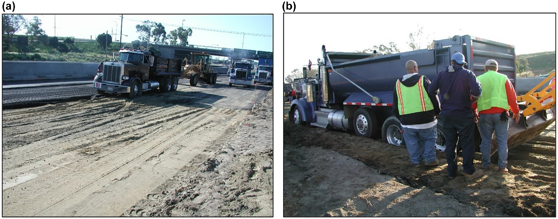
(a) Note asphalt paved directly on subgrade, (b) Note extensive damage to the subgrade.

The characterization of the subgrade and subbase layers can be complex and often has the least attention paid to it in design. It is common to spend tens of thousands of dollars characterizing the asphalt concrete for a design while using a visually rated soil classification to obtain default properties for the subgrade. Again, this is less of an issue for rehabilitation since the subgrade can be characterized by deflection testing and back-calculation, but it is not always possible to perform extensive laboratory or field testing of the subgrade for new pavements, as is suggested in NCHRP 1-37A ( 1 ). Frequently design methods assume an adequate construction platform.

This paper presents a proposed approach for construction platform design based on the DCP-DN design method ( 2 ). The Dynamic Cone Penetrometer (DCP) has been used worldwide since the 1960s to determine the strength of the top ∼800 mm of unbound granular layers in a pavement. The DCP is a straightforward tool that uses a hammer (with a known weight and drop height) to drive a cone through the soil while measuring the penetration depth after each blow. The penetration rate is measured as DN, the abbreviation of “DCP Number” used in the South African literature, therefore the DCP-DN method. It can be used to determine a strength profile with depth and is reasonably well correlated with the field California bearing ratio (CBR), resilient modulus (M_R), unconfined compressive strength (UCS) and other properties of the material. In the U.S.A., the penetration rate is often referred to as DCP penetration index (DPI), but is still reported in millimeters per blow, a convention followed here. Other authors use the abbreviations PR (penetration rate) or PI (penetration index) and will occasionally use thousandths of an inch (mils) per blow.

To tie the DCP-DN and a mechanistic-empirical (ME) design together, a relationship to convert between DPI and M_R is required. Many relationships have been published in the literature, with some discussion about which one is “right” when none are strictly correct. However, using meta-analysis techniques, combining these published relationships to determine an overall best fit is possible, allowing other properties to be used for the DCP-DN method and the DCP data for design. Thus, this paper also presents a meta-analysis of published relationships to obtain DPI and the other properties listed above (especially M_R).

Background

Design methods can be broadly classified into empirical and ME, with the latter currently receiving most of the research focus. Most empirical methods build on the long tradition of “cover” based designs, including the California R-value method, the AASHTO structural number concept, and the USACE CBR cover curves. These methods codify empirical observations of pavement performance, and what they all have in common is that a particular subgrade requires a certain cover to handle the traffic adequately and that better quality materials (such as aggregate base compared with imported borrow) contribute more cover per unit thickness.

In ME design, the method analyzes critical responses in the pavement and uses these as latent variables in empirical (i.e., statistical) transfer functions to determine performance. One of the downsides to ME design is that it can analyze any pavement structure, so this concept of cover is implicit, and it is possible to design structures that perform adequately but are not ideal. For example, one can design a full-depth asphalt pavement on a very soft subgrade or design a thick Portland Cement Concrete (PCC) slab on the same soft subgrade. In both cases, most ME design methods will show reasonable results for low to medium traffic. However, these pavements will not perform well because of distress mechanisms not captured by the design method. In addition, they will be difficult or impossible to construct. In the case of the flexible pavement, it will be impossible to compact the bottom lift of the asphalt layer to the required density, and in both cases, it will be likely that construction traffic will get stuck and rut and deform the subgrade before the upper layers can be built.

It is thus essential to have some method to enforce the lesson of cover and ensure an adequate construction platform within an ME design method. Some methods specify the minimum index properties (e.g., grading and plastic index) of materials for the construction platform (especially in catalogs of designs based on ME analysis). However, if the in-situ materials are not within these minimum specifications but might still be adequate, this can result in additional cost. The insight of this work is that there exists an entire set of empirical design methods for low-volume roads of various kinds, such as unpaved roads, forest roads, mine haul roads, or roads in developing countries and rural areas. If the construction platform is viewed as a low-volume road designed to handle the construction traffic, then one of these methods can be used to design the lower layers.

An alternative approach would be to incorporate construction traffic loading on each layer directly into the ME design method. While this would be feasible, it might require several additional damage models, each requiring calibration, and other changes which might be difficult to implement. In addition, it would require estimation of the construction traffic on each layer.

The DCP-DN Design Method

The DCP is a well-documented test that is well known to most pavement engineers ( 3 ), so it will not be detailed here. However, less well known is that the DCP can be used directly for pavement design. The DCP-DN design method originated in South Africa ( 4 ), where the DCP is widely used. The method was validated with extensive field observations, combined with heavy vehicle simulator tests, to determine the structural capacity of the pavements, and is currently used widely within Africa for low-volume road design, as detailed in a recent review by Paige-Green and Van Zyl ( 2 ), which provides extensive background to the history and development of the method, along with comparisons with other design methods. Fundamentally, the DCP-DN method builds on the long tradition of cover-based designs by taking the field measured DCP profile and comparing it with an idealized profile, and then requiring the addition of one or more cover layers to ensure the resulting post-construction DCP profile would meet or exceed the required idealized profile.

The DCP-DN design method has two differences from other empirical design methods that are beneficial if we only consider the lower unbound granular layers in a pavement. The first is that it uses the overall strength of the top ∼800 mm of unbound material, characterized by the total number of blows to reach a depth of 800 mm (DSN₈₀₀), rather than just a single subgrade surface measurement. The second is that the method explicitly relies on an additional concept of pavement “balance.” Balance has two components: a type of structure and how well the pavement fits that structure. A “deeply” balanced pavement has successively stronger/stiffer layers on top of weaker/softer ones so that the ratio between successive layers is not too high. One with a “shallow” balance has a high ratio between the respective layers, meaning that the bottom of each layer tends to be in tension, and an “inverted” structure has weaker layers on stiffer layers. One property that can be determined for each DCP result (as long as the penetration depth is at least 800 mm) is the balance number (B), which measures the non-uniformity of the penetration rate with depth and is obtained by fitting the standard pavement balance curve, shown in Equation 1, to the penetration data ( 5 , 6 ).

BS N_{d} = \frac{DS N_{800}}{100} \frac{d (400 B + {(100 - B)}^{2})}{4 Bd + 8 {(100 - B)}^{2}}

(1)

where

BSN_d = number of blows to reach depth d,

DSN ₈₀₀ = number of blows to reach a depth of 800 mm,

d = penetration depth (mm),

B = balance number.

Deeply balanced pavements are defined as having B values from 0 to 40, shallow structures have B values greater than 40, and inverted structures have B values less than zero ( 6 ). For each of these three types of structure, a “well-balanced” pavement follows the balance equation closely (so that the modular ratio remains relatively constant with depth), while “averagely” and “poorly” balanced pavements have progressively higher deviations from the standard balance curve.

Balance is vital for a construction platform because strength and stiffness are a function of density, and density is a function of compaction energy. Without a good construction platform to act as an “anvil,” one cannot impart this energy into the layer being compacted, and it will instead be absorbed by the layers below. This implies that the construction platform can only be built using a deeply balanced design from bottom to top (i.e., 0 ≤ B < 40). A balance number (B) of 30 to 40 would be ideal if one had access to good quality borrow or subbase material because it would allow the thinnest added layers, reducing cost. However, there is a trade-off: the higher the balance number, the harder it is to achieve compaction of the added layers. Unlike other empirical methods, the DCP-DN method allows the designer to explore this relationship in design and choose a B value that works both in the DCP-DN method and in the ME design, accommodates locally available materials, and the field measured DCP profile. Shallow and inverted designs can generally only be achieved using mechanical stabilization.

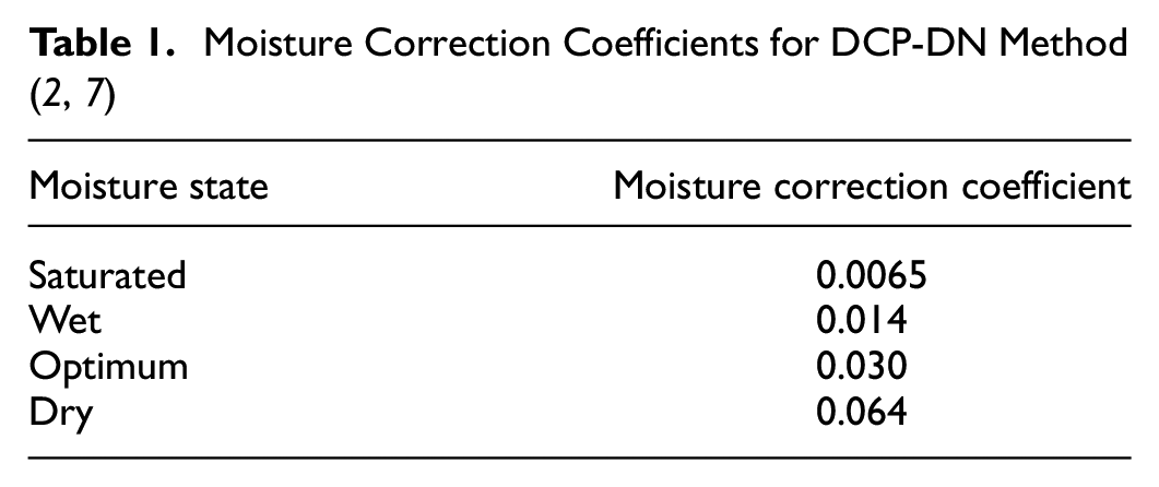
The DCP-DN design method correlates performance, measured as allowable single-axle load equivalents (ESALs) to DSN₈₀₀ from the DCP test. A correction is applied for different moisture levels in the pavement (saturated, wet, optimum, or dry) see Table 1. Given design traffic and moisture conditions, a required DSN₈₀₀ can be calculated as follows ( 2 , 4 ):

DS N_{800} = {(\frac{ESAL}{C})}^{\frac{1}{3.5}}

(2)

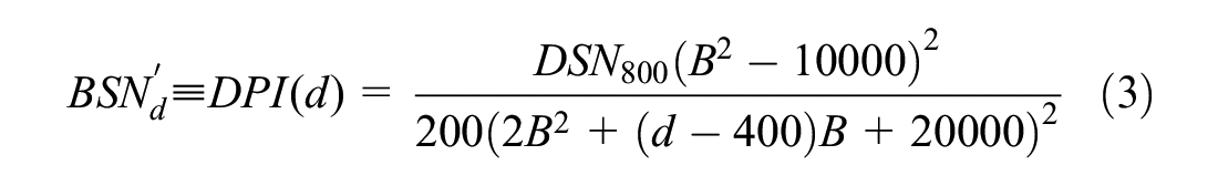
If DCP test data are available, B from the data can be used, or B can be chosen—either way, a profile of blow count to depth is determined with these two parameters. The derivative of this profile gives the required DPI profile with depth:

{BSN}_{d}^{'} \equiv DPI (d) = \frac{DS N_{800} {(B^{2} - 10000)}^{2}}{200 {(2 B^{2} + (d - 400) B + 20000)}^{2}}

(3)

This profile can also be seen as a required in-situ CBR, R-value, or $M_{R}$ at each depth with a suitable conversion. Note that choosing DSN₈₀₀ and B fixes the DPI at the surface, which is equivalent to specifying a minimum subgrade CBR or R-value. Similarly, by making assumptions about the material below 800 mm, one could compute a subgrade elastic deflection or a modulus of subgrade reaction (k-value). The profile with depth becomes the target penetration curve for a DCP test. If the field measured penetration curve is weaker at any depth than this, layers are added (with assumed DPI based on the material) until the curve is satisfied. In the case of the construction platform, one would only be adding borrow or subbase materials.

Table 1.

Moisture Correction Coefficients for DCP-DN Method ( 2 , 7 )

Moisture state	Moisture correction coefficient
Saturated	0.0065
Wet	0.014
Optimum	0.030
Dry	0.064

One assumption of the DCP-DN method is that the road has a seal coat ( 2 ), which is unlikely to be true of a construction platform. However, a seal coat provides minimal structural capacity and mainly limits moisture ingress and surface wear. Most construction vehicles use specialized tires and low inflation pressures, so some of the concerns around the performance of the top ∼25 mm of the pavement are not relevant in this case. In addition, construction traffic on the lower layers is not channelized by lane markings.

To use this design method, one needs to know the DPI for each type of cover material that could be used, which prompts the development of a consistent correlation between DPI and various other soil properties that are typically available, because DPI is often only available for in-situ materials. At a minimum, this requires representative DPI values for different soil classifications, but if other laboratory-measured properties (such as CBR or R-value) are known, these can be used to estimate the penetration rate. In addition, the moduli for these materials would also need to be estimated for ME design, likely using similar methods. Conversely, if an ME design is being considered, the moduli can be converted to DPI to determine a pseudo penetration curve for the lower layers, which can be checked to ensure the construction platform is adequate. Nearly every ME design method has built-in default moduli values for various materials. In many cases, relationships to other properties are also provided, such as in the Guide for Mechanistic-Empirical Design of New and Rehabilitated Pavement Structures ( 1 ), because the determination of properties for unplaced materials in a design method has always been a problem. Many design methods include these relationships, which leads directly to the question of what relationships to use.

Meta-Analysis of Relationships Between Subgrade Strength and Stiffness Properties

Over the last 60 years, since the 1960s, many relationships between various strength and stiffness parameters for soils have been published, along with typical ranges for various soil types, and new studies are still being published. Typically, these papers or reports cite a few “authoritative” sources for the relationship in question, reproduce the same figures and descriptions of well-known test methods, and then have some new data to develop a new relationship, which is then compared with those already published. In nearly all cases, the authors find a similar relationship with slightly different parameters, and the reader is left to choose if they prefer the new relationship to the old, and since the old is published in a standard, it continues to be used. It is also common to see the various nomographs that allow one to graphically convert between two or more properties reproduced, and either a table or graph of typical ranges for AASHTO and Unified Soil Classification (USC) classes (which are typically not updated by the authors). Most of the fitted models are done independently, so one is cautious about using a new correlation to obtain CBR from DPI but then using an old nomograph to convert CBR to M_R. As a result, even the newest design methods still use correlations developed in the 1960s and 1970s ( 1 ).

What is needed is a way to combine these studies and harmonize the conversions between all the properties. If the raw data and exact methodologies from all these studies were available, it would be possible to develop an extensive data set and perform a comprehensive statistical analysis, including joint estimation of all relationships simultaneously. However, data are not available for many studies (or would have to be digitized off plots). Faced with a similar problem, it has become quite common recently for researchers in other fields to turn to Bayesian meta-analysis ( 8 ), which allows each published model to be treated as a data set with sampling error. This requires a complete set of statistical parameters, however, these are not published in most cases.

As a last resort, a simple meta-analysis is possible by using only the published relationships. The type of data and problem domain here are not typical of meta-analyses found in other scientific literature, so a new methodology was developed. Firstly, working on the assumption that the published models are well formulated, each represents the best estimate of both the mean and the median (i.e., 50% percentile) of the data at any particular input value. However, because the models tend to be extrapolated past the test data, we are likely to encounter outliers at the edges of the range. For this reason, a least absolute deviation (LAD) solution is preferred over the more common ordinary least-squares approach because it is robust against outliers. This approach will fit the median value from the model predictions rather than the mean. In addition, the approach needs to consider the joint estimation of parameters across all the various combinations of properties so that the complete set of models is self-consistent with the underlying published models (and, therefore, hopefully, the original data).

For simplicity, we will only consider single input conversion models, not those requiring multiple inputs, making the results more general, but excluding those that require additional information like plasticity index or other numerical inputs. While some relationships might be specialized to a particular soil type (such as high or low plasticity clays), the other relationships are typically not specialized in this way, meaning that two-step (e.g., DPI to CBR to M_R) relationships might be biased. Also, every additional constraint limits the usefulness when that condition is not known in advance.

If we have $M$ properties, numbered $m = 1 . . M$ , there are $N_{p}^{m}$ published models per property combination $(m, p)$ with $m \in (1, M - 1)$ and $p \in (m + 1, M)$ . Each published model $x^{p} = F_{n}^{mp} (x^{m})$ has a valid range of $x_{n}^{mp} \in (a_{n}^{mp}, b_{n}^{mp})$ . To ensure internal consistency, there must only be $M - 1$ fitted models $x^{M} = f_{m} (x^{m}, α_{m})$ each relating property $m$ to property $M$ , with parameters vectors $α_{m}$ , and the remaining models must be formulated as transforms via property $M$ so:

x^{p} = f_{p}^{m} (x^{m}, α_{m}, α_{p}) \equiv f_{p}^{- 1} (f_{m} (x^{m}, α_{m}), α_{p})

(4)

Because all the properties are on different scales, the error formulation would naturally be complex to account for unit differences. However, we have one advantage: most published models of interest are log-log models. This means that their errors are ratios, making all the errors for different properties equivalent. The only property of interest that does not fall into this mold is the California R-value, which is often not transformed. 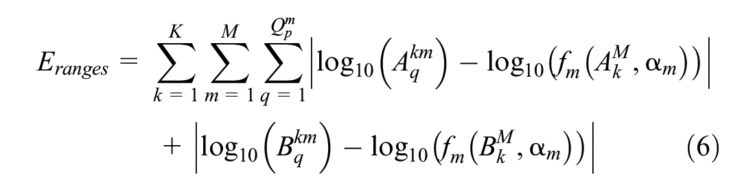R-value is constrained to a range of zero to 100, so the transform $atanh (R / 100)$ was chosen, and since it is always the input property in the combinations of published models, it is never considered in the error.

The error can be formulated as:

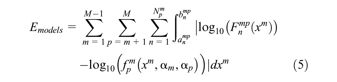
E_{models} = \sum_{m = 1}^{M - 1} \sum_{p = m + 1}^{M} \sum_{n = 1}^{N_{p}^{m}} \int_{a_{n}^{mp}}^{b_{n}^{mp}} | \log_{10} (F_{n}^{mp} (x^{m})) - \log_{10} (f_{p}^{m} (x^{m}, α_{m}, α_{p})) | d x^{m}

(5)

The integral in the error function can be replaced by a few sample points, and the error summed over these without significant loss of accuracy. An added aspect of error minimization also includes the errors from the published minimum/maximum ranges of properties for various soil types. If we have $K$ soil classifications, with $Q_{k}^{m}$ published ranges for each property, where the ranges are $(A_{q}^{km}, B_{q}^{km})$ and $(A_{k}^{M}, B_{k}^{M})$ is a trial range for property $M$ of soil classification $k$ , then this error can be formulated as:

E_{ranges} = \sum_{k = 1}^{K} \sum_{m = 1}^{M} \sum_{q = 1}^{Q_{p}^{m}} | \log_{10} (A_{q}^{km}) - \log_{10} (f_{m} (A_{k}^{M}, α_{m})) | + | \log_{10} (B_{q}^{km}) - \log_{10} (f_{m} (B_{k}^{M}, α_{m})) |

(6)

Statistically, the two models can be seen as specialized joint LAD estimators. The sum of these two functions can be jointly minimized with respect to the parameters and ranges to obtain the best fit. Using these results, it is also possible to construct an updated nomograph that can be used for quick visual estimation of properties.

There is no way to test goodness-of-fit because there are no observations to plot against or use in the determination of $r$ -squared or $p$ -values, besides which these are not appropriate for a LAD estimator. However, the main reason for considering $p$ -values is to determine which explanatory variables to include in a model and compare different model forms. In this case, most of the literature uses the same model forms for various property combinations, so it is reasonable to use them if multiple researchers have found them to be best for their data. In addition, each model only has one variable, which multiple researchers have found to be significant, so there is no real question of validating its use in the model, only rejecting the relationship between the two properties completely.

Meta-Analysis Results

While direct measurement of properties is always desirable, there are cases where estimating one property from another is necessary. The goal of this meta-analysis is not to perpetuate the idea that one can visually assess the subgrade soil classification and determine all the required properties without testing but to act as a “test of reasonableness” to cross-check other testing or provide guidance when testing cannot be performed (for example, when the material does not yet exist). If additional information about the soil is available (such as alluvial versus residual soils), a locally developed correlation specific to that soil type might provide better estimates. However, if one were, for example, to use a local relationship to obtain DPI from CBR, then use the models presented here to convert to stiffness, there would be little benefit over converting directly from CBR to stiffness.

Since an elastic modulus is required for all ME design methods, this was chosen as the reference property in the meta-analysis (property $M$ ). The other properties that frequently appear in the literature are the DPI (with 30° and 60° cones), three CBRs (soaked, laboratory/unsoaked, and in-situ/field), R-value, UCS, Standard Penetration Test (SPT) blow counts using a split tube sampler, and subgrade reaction modulus (known as the k-value). In total, 126 published relationships between these properties and five tables of expected ranges for various soil classifications were found. The model forms and parameters for all 126 models are not republished here, but every effort has been made to track the original references and check the values. A model was fitted to published data in a few cases when the model coefficients were not given in the original work but the raw data were supplied.

Every attempt has been made to remove duplicate models, especially those with the same parameters when expressed in SI units. In some cases, the published coefficients are rounded versions of those found in their citations. For example, the common relationship for $M_{R}$ (in pounds per square inch [psi–>) = 1,500 CBR typically cites Heukelom and Klomp ( 9 ), but actually derives from Heukelom and Foster ( 10 ), republished as Heukelom and Foster ( 11 ), and the original has the unusual unit of kilogram force per square centimeter, so is actually $M_{R}$ (in kg/cm²) = 110 CBR, or $M_{R}$ (in psi) = 1546.6 CBR. This relationship is also often quoted, with the same citation, as $M_{R}$ (in MPa) = 10 CBR when the original would be 10.8 and psi conversion from 1,500 would be 10.3. Now, none of these is any better or worse because they are all within reason given the noise in the original data (and since “10 times the CBR” is an easy to remember heuristic), but this equation should only be included once in the meta-analysis, using the original formulation. However, if some duplicates remain, it does not invalidate the analysis, only bias it slightly toward these models.

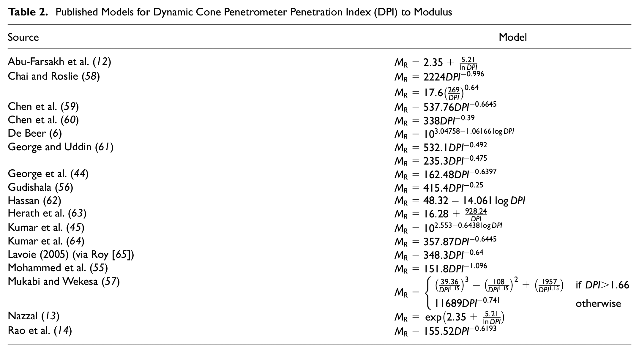
Figures 2 to 4 show the 126 published models (restricted to their valid ranges when possible). In each plot, the median for the published models is shown using large gray circles, and the final fitted model is shown using a thick black line. The other lines show the various published models. References are provided for each of the models on the figure. In some cases, the model needed to be inverted to be plotted or converted to SI units. A correction for the Australian standard 30° DCP cone to the more common 60° cone is used to correct the fitted model. While the DCP and CBR values have been split out, the modulus values have not been split by test type or other features, because in many cases, the test method was not given. Models with different constraints and limits (e.g., sand or clay specific) are also included without limiting the analysis to match these constraints. Some studies have multiple models fitted to the data, using different subsets. For these studies the most general published model is used, but if two or more models are published then all are included as separate models.

Figure 2.

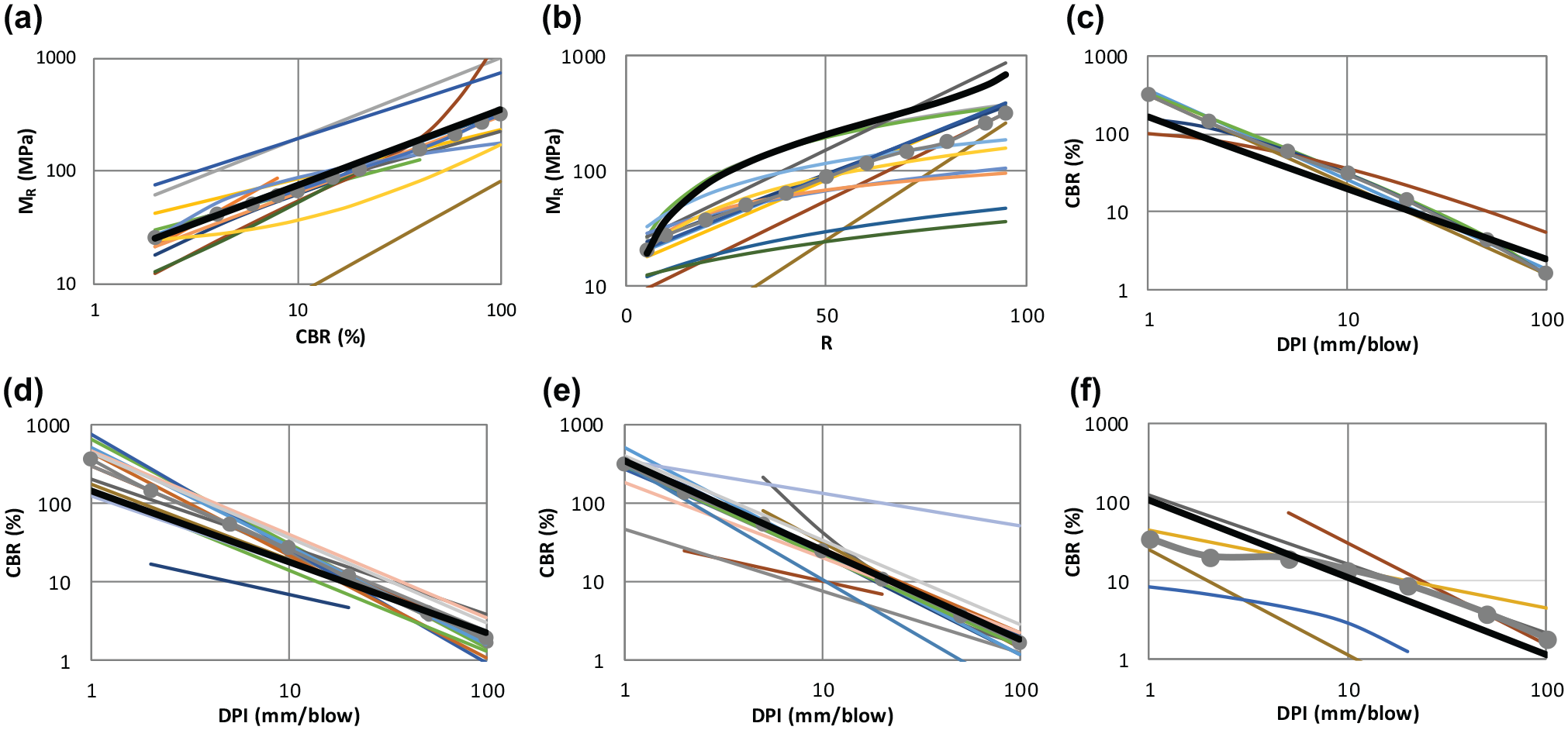
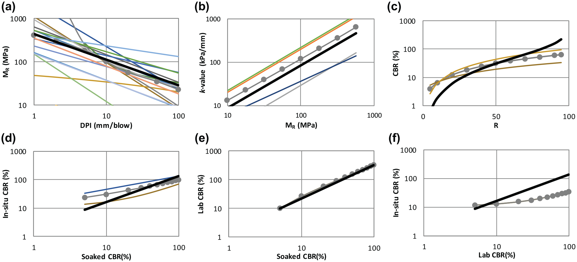
Plots of various published models along with the overall best fit model: (a) CBR versus $M_{R}$ ( 9 – 24 ), (b) R-value versus $M_{R}$ ( 1 , 25 –30), (c) 30° cone DPI versus in-situ CBR ( 31 – 34 ), (d) DPI versus in-situ CBR ( 23 , 24 , 35 –43), (e) DPI versus lab CBR ( 5 , 13 , 19 , 23 , 36 , 44 –53), and (f) DPI versus soaked CBR ( 39 , 46 , 50 , 54 ).

Figure 3.

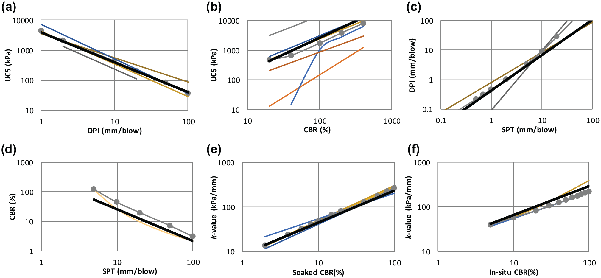
Plots of various published models along with the overall best fit model: (a) DPI versus $M_{R}$ ( 6 , 12 –14, 44 , 45 , 55 –65), (b) $M_{R}$ versus k-value ( 1 , 66 –68), (c) R-value versus soaked CBR ( 69 ), (d) soaked versus in-situ CBR ( 16 , 24 , 70 ), (e) soaked versus lab CBR ( 24 ), and (f) lab versus in-situ CBR ( 24 ).

Figure 4.

Plots of various published models along with the overall best fit model: (a) DPI versus UCS ( 5 , 50 , 57 , 71 ), (b) CBR versus UCS ( 19 , 72 –75), (c) SPT versus DPI ( 76 , 77 ), (d) SPT versus CBR ( 35 , 78 ), (e) soaked CBR versus k-value ( 79 ), and (f) in-situ CBR versus k-value ( 69 , 80 , 81 ).

Table 2 shows the 19 published models for Figure 3a. As can be seen, most of the models are exponential, so log-log when linearized, with slopes around negative one half and a scale of between 100 and 1,000 MPa, implying an intercept of 2–3 in log₁₀ space. The equation by Mohammed et al. ( 55 ), shown as a light green line on the bottom left in the figure, seems to be an outlier with a low intercept and high negative slope, as does that of Gudishala ( 56 ), shown as a light blue line in the top right, which has a reasonable intercept but low slope. In addition, the model by Mukabi and Wekesa ( 57 ), the almost vertical curving gray line, seems to have some interesting behavior and is probably not benefiting from the complex formulation. However, when we take the median value of the model predictions (the gray circles), we obtain a relatively straight line with a modulus of around 400 MPa at 1 mm/blow (which would be reasonable for a well-compacted granular base) and almost exactly 100 MPa at 10 mm/blow, which again would be reasonable for subgrade material. These median points are not used in the model, but this relationship has many underlying models, so, naturally, the overall best fit follows the median closely. As expected, the overall best fit (Equation 10) has coefficients that fall within those for the published models. The residual absolute difference is 0.347 orders of magnitude for this relationship, implying that the model predictions could be 2.2 times too high or low. Since this does not include the residual error from the underlying studies’ data, the actual residual standard deviation for predictions would be higher than this.

Table 2.

Published Models for Dynamic Cone Penetrometer Penetration Index (DPI) to Modulus

Source	Model
Abu-Farsakh et al. ( 12 )	$M_{R} = 2.35 + \frac{5.21}{\ln DPI}$
Chai and Roslie ( 58 )	$M_{R} = 2224 DP I^{- 0.996}$
Chai and Roslie ( 58 )	$M_{R} = 17.6 {(\frac{269}{DPI})}^{0.64}$
Chen et al. ( 59 )	$M_{R} = 537.76 DP I^{- 0.6645}$
Chen et al. ( 60 )	$M_{R} = 338 DP I^{- 0.39}$
De Beer ( 6 )	$M_{R} = 10^{3.04758 - 1.06166 \log DPI}$
George and Uddin ( 61 )	$M_{R} = 532.1 DP I^{- 0.492}$
George and Uddin ( 61 )	$M_{R} = 235.3 DP I^{- 0.475}$
George et al. ( 44 )	$M_{R} = 162.48 DP I^{- 0.6397}$
Gudishala ( 56 )	$M_{R} = 415.4 DP I^{- 0.25}$
Hassan ( 62 )	$M_{R} = 48.32 - 14.061 \log DPI$
Herath et al. ( 63 )	$M_{R} = 16.28 + \frac{928.24}{DPI}$
Kumar et al. ( 45 )	$M_{R} = 10^{2.553 - 0.6438 \log DPI}$
Kumar et al. ( 64 )	$M_{R} = 357.87 DP I^{- 0.6445}$
Lavoie (2005) (via Roy [ 65 ])	$M_{R} = 348.3 DP I^{- 0.64}$
Mohammed et al. ( 55 )	$M_{R} = 151.8 DP I^{- 1.096}$
Mukabi and Wekesa ( 57 )	$M_{R} = {\begin{matrix} {(\frac{39.36}{DP I^{1.15}})}^{3} - {(\frac{108}{DP I^{1.15}})}^{2} + (\frac{1957}{DP I^{1.15}}) & if DPI > 1.66 \\ 11689 DP I^{- 0.741} & otherwise \end{matrix}$
Nazzal ( 13 )	$M_{R} = \exp (2.35 + \frac{5.21}{\ln DPI})$
Rao et al. ( 14 )	$M_{R} = 155.52 DP I^{- 0.6193}$

In most cases, the overall best fit is close to the median for the published models. However, there are some cases where it differs considerably. In Figure 2b, the R-value follows the upper edge of the published models for most of the M_R range, which corresponds to the model in the AASHTO 1993 design method ( 66 ), ignoring the majority of the published models. It is unclear why this is the case, but it appears necessary for the other correlations (such as CBR) to fit. Overall, the fitted model makes sense, and the relationships are well within the expected ranges. The following equations give the final relationships:

\log_{10} (M_{R}) = 1.211 + 0.665 \log_{10} (CB R_{i})

(7)

\log_{10} (M_{R}) = 1.319 + 0.525 \log_{10} (CB R_{u})

(8)

\log_{10} (M_{R}) = 1.416 + 0.608 \log_{10} (CB R_{s})

(9)

\log_{10} (M_{R}) = 2.646 - 0.595 \log_{10} (DPI)

(10)

M_{R} = 380.6 atanh (R / 100)

(11)

\log_{10} (M_{R}) = 0.489 + 0.599 \log_{10} (UCS)

(12)

\log_{10} (M_{R}) = 2.867 - 0.715 \log_{10} (SPT)

(13)

\log_{10} (M_{R}) = 0.037 + 1.013 \log_{10} (k)

(14)

The equations above are all based on the SI units shown on the nomograph (and other figures). Confidence intervals are not supplied because they would need to include the residual errors from the underlying models, which are not available in many cases. However, the overall residual absolute error is 0.264 orders of magnitude or ±1.8 times. In other words, the error of any particular prediction of M_R from these equations is probably within a factor of two of the actual modulus. The DCP/CBR relationships tend to be more tightly clustered, hinting that these two tests are probably measuring similar properties (which is not surprising). The modulus relationships tend to have a larger range (of up to an order of magnitude on both sides in some cases), indicating that the relationship between the shear/strength properties and stiffness is more tenuous (which is also no surprise). The error in the minimum-maximum values for the classifications is 0.13 orders of magnitude or a factor of 1.3. The error here is probably lower because most of the published ranges of various properties are already highly curated and probably do not reflect the full range of values seen in the field.

Using these equations, and the ranges for the various soil classifications, the nomograph shown in Figure 5 can be created, by taking a range of values for each property, converting these into M_R and plotting an axis. Additional axes are added for U.S. customary units for properties where these are used. The nomograph provides a quick visual method to cross-check various parameters and can be read by finding a given value on the scale of interest and projecting vertically up or down to the other scales to find the corresponding values. In addition, two sets of ranges are given for the AASHTO and USC systems, which can be used to obtain reasonable ranges for the various properties if only the classification is known.

Figure 5.

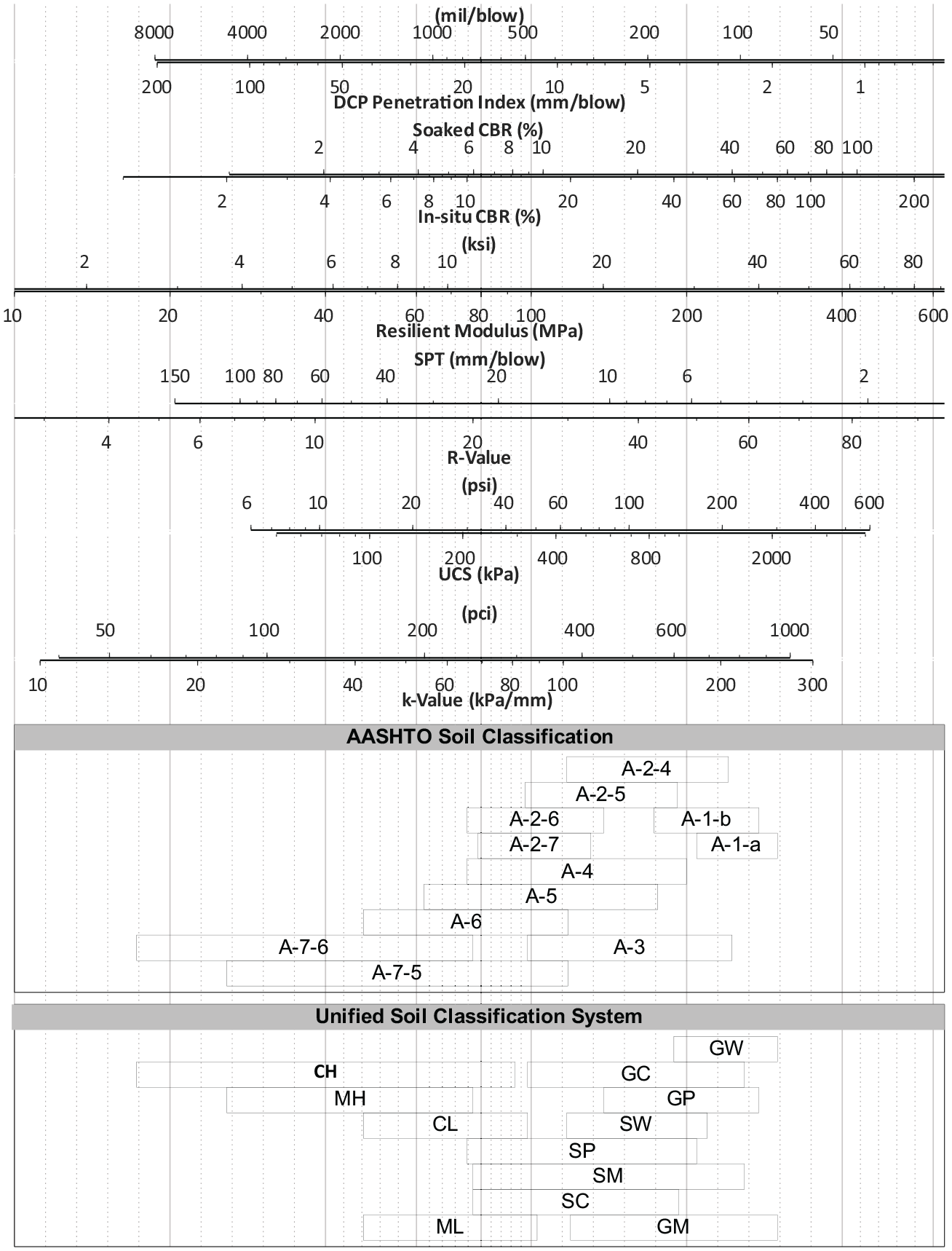
Nomograph based on overall best fit model.

Application of the DCP-DN Design Method

The actual application of any low-volume road design method to the design of the construction platform would typically depend on the agency responsible and the context and would need to accommodate existing practice. However, two examples of how the DCP-DN design method might be used in the ME design of new pavements are given below. Since the goal is not to replace the ME design of the lower layers but still to ensure an adequate platform by constraining the designer, we can be conservative in the assumptions—a well-specified ME design method will respond to the improved subgrade/subbase by allowing thinner base and surface layers, so the cost of the overall design should be comparable.

The first example might be for a greenfield design for a new large highway. We will assume the construction platform is soaked and a construction traffic load of 1,000 ESALs (this assumes that the platform will be exposed to considerable construction traffic—equivalent to hauling enough aggregate base for ∼20 lane-km of construction). A B value of 38, at the top end of the deeply balanced range, is appropriate for granular layer construction since it builds the layers as thin as possible while maintaining adequate cover. Based on these assumptions and Equation 2, the subgrade requires a DSN₈₀₀ of 31 (31 blows to reach 800 mm, or about one blow per inch). Using B and Equation 3, we can obtain the required profile shown in Figure 6.

Figure 6.

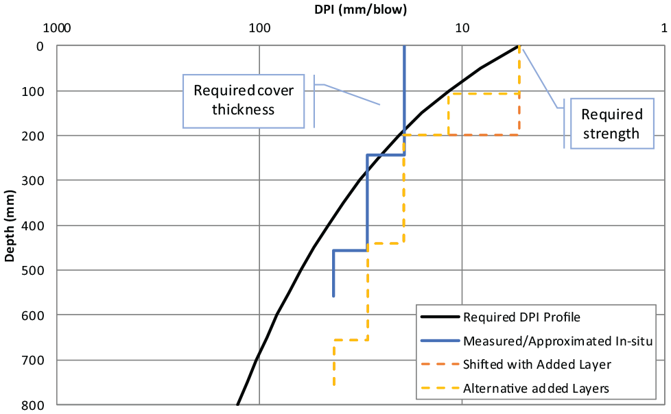
Required minimum dynamic cone penetrometer penetration index (DPI) profile with depth and cover.

Any measured stiffness profile that falls to the right of this curve will have a DSN₈₀₀ of at least 31 but will likely have a different B. Unlike some cover-based design methods, the DCP-DN based design essentially specifies the minimum required stiffness at the surface, so it is insufficient to cover a weak subgrade with a thick layer of better, but still not strong, material (like an imported borrow). If DCP testing can be performed at the site, a layer strength diagram could be obtained from the DCP analysis. In this example, the profile has a 245 mm layer with a DPI of 20 mm/blow, followed by a 200 mm layer at 30 mm/blow and 45 mm/blow below that, shown in Figure 6 as the measured profile. From this, we can determine both the depth of cover and the required stiffness of the cover. These are also shown in Figure 6. In this example, the top layer of the measured profile is the limiting point and requires ∼200 mm of cover to meet the profile, with a material with a DPI of <5 mm/blow (which, based on the nomograph, would have CBR∼22 and M_R∼170 MPa). However, we do not need to use this material through the entire cover layer. We could use two 100 mm layers, with the lower having a DPI of ∼11 mm/blow. The appropriate strategy would depend on the availability of material and other factors.

A second example might be a two-lane rural access road with a deep clay subgrade in a river delta. In this case, we might only obtain a single measurement, that the subgrade has a modulus of ∼25 MPa, based on triaxial testing, which would correspond to a material with a soaked CBR of less than one or a DPI of ∼125 mm/blow, which should raise some concern. A pure ME design on this material suggests that a 240 mm polymer-modified full-depth asphalt layer would be sufficient for a 20-year design. However, using construction traffic of just 20 ESALs (and the same B of 38), a DSN₈₀₀ of 10 would be required, along with a surface DPI of ∼16 mm/blow (corresponding to a material with a CBR of ∼7 and stiffness of ∼85 MPa) which would be in line with an imported borrow in most standards. A cover depth of 300 mm would be needed. The same ME design method now shows that the full-depth asphalt layer could be reduced to 210 mm. Of course, a full-depth asphalt might not be the best strategy here, and the ME design shows that placing a 150 mm aggregate base on the imported borrow would allow the asphalt to be further reduced to 180 mm.

Applying the same 1,000 ESALs requirement from the first example to the second would require 800 mm of cover, with the same requirement of ∼170 MPa for the top layer of the cover, with at least 150 mm of this material over 650 mm of the imported borrow, which would probably be more in line with a typical state highway design for such a poor subgrade.

This procedure can be implemented in an ME design method by considering the layers in the design, checking if the lower layers are granular materials, and converting their reference modulus values to DPI, using Equation 10. The balance number (B) and ESALs can be hard-coded or inputs provided, but these are used to establish the required DPI profile. If the profile is not met, a warning can be shown to the user, requiring them to insert a borrow or subbase layer. These checks can be integrated with the other checks, such as minimum and maximum layer thicknesses, moduli, and others.

The best method for establishing an existing stiffness profile with depth at a site is through DCP testing because this provides a field measurement at various depths. Because it is relatively quick and easy, it also allows many tests to be run at different locations, allowing a much better spatial coverage than triaxial testing. The DCP data can also be used to segment the subgrade into uniform segments, and the cover thickness adjusted based on the measurements within each segment. In addition, the DPI can be used to estimate the subgrade stiffness.

However, if a full profile with depth is not possible, then using a single value to characterize the subgrade is acceptable if it can be established that the sample represents the weakest layer. A depth profile should be developed if the in-situ condition has a stiffer layer on a weak layer (for example, from an existing imported layer).

Conclusion and Recommendations

This paper shows that it is possible to use a low-volume road design method to specify the lower layers of a pavement designed using a modern ME method to ensure that it has an adequate foundation and a suitable construction platform. The DCP-DN design method was chosen because it is easy to apply and has the advantage over other methods that it utilizes the strength profile of the subgrade. In addition, the DCP results can be used to characterize the subgrade for ME design as an alternative/supplement to traditional geotechnical tests and laboratory testing. Because the DCP is a quick and simple test, more testing can better capture subgrade variability or anomalies.

In addition, this paper presents a meta-analysis of many published correlations between DPI, $M_{R}$ , and other common properties, allowing other methods of characterizing the subgrade to be used if DCP testing is not possible. These relationships can also be used to obtain materials and parameters for input into an ME design. By using a meta-analysis, the best fit to all the published models can be obtained, resulting in a new set of internally consistent relationships between these properties.

The meta-analysis could be extended to other soil properties of interest. Some published relationships relating the existing properties to shear strength and the Cone Penetrometer Test were not included. In addition, there is a large body of work not explored here that relates the various properties on the nomograph to intelligent compaction parameters. A valuable extension to this work would be to correlate DSN₈₀₀ with some parameters from intelligent compaction so that it would be possible to specify a minimum roller response to ensure an adequate construction platform.

Footnotes

Acknowledgements

The authors appreciate the technical review by staff of California Department of Transportation (Caltrans), especially Raghubar Shrestha, Office of Asphalt Pavements, and oversight by Joe Holland, of the Division of Research, Innovation and System Information. The assistance of Biana Giang in collecting the citations is also gratefully appreciated.

Author Contributions

The authors confirm contribution to the paper as follows: study conception and design: J. D. Lea, R. Wu, J. T. Harvey; data collection: J. D. Lea; analysis and interpretation of results: J. D. Lea; draft manuscript preparation: J. D. Lea. All authors reviewed the results and approved the final version of the manuscript.

Declaration of Conflicting Interests

The author(s) declared no potential conflicts of interest with respect to the research, authorship, and/or publication of this article.

Funding

The author(s) disclosed receipt of the following financial support for the research, authorship, and/or publication of this article: This paper describes research activities requested and sponsored by the California Department of Transportation (Caltrans) Grant #65A0788.

ORCID iDs

Jeremy D. Lea

Rongzong Wu

John T. Harvey

Data Accessibility Statement

The database and code for this paper will be published at , where others can contribute additional models or properties.

The contents of this paper reflect the views of the authors and do not necessarily reflect the official views or policies of the State of California or the Federal Highway Administration. This paper does not represent any standard or specification.

References

ARA Inc., ERES Consultants Division. Guide for Mechanistic-Empirical Design of New and Rehabilitated Pavement Structures. Final report, NCHRP Project 1-37A. Transportation Research Board of the National Academies, Washington, D.C., 2004. http://www.trb.org/mepdg/guide.htm.

Paige-Green

Van Zyl

G. D.

A Review of the DCP-DN Pavement Design Method for Low Volume Sealed Roads: Development and Applications. Journal of Transportation Technologies, Vol. 9, No. 4, 2019, pp. 397–422. https://doi.org/10.4236/jtts.2019.94025.

ASTM D6951/D6951M-18. Standard Test Method for Use of the Dynamic Cone Penetrometer in Shallow Pavement Applications. ASTM International, West Conshohocken, PA, 2018.

Kleyn

E. G

. Aspects of Pavement Evaluation and Design as Determined With the Aid of the Dynamic Cone Penetrometer. M.Sc. thesis. University of Pretoria, South Africa1984.

Kleyn

E. G.

The Use of the Dynamic Cone Penetrometer (DCP). Report L2/74. Transvaal Roads Department, Materials Branch, Pretoria, South Africa, 1975.

De Beer

. Use of the Dynamic Cone Penetrometer (DCP) in the Design of Road Structures. Maseru, Lesotho, 1991.

Marais

G. P.

Maree

J. H.

Kleyn

E. G.

The Impact of HVS Testing on Transvaal Pavement Design. Pretoria, South Africa, 1982.

Gronau

Q. F.

Heck

D. W.

Berkhout

S. W.

Haaf

J. M.

Wagenmakers

E.-J.

A Primer on Bayesian Model-Averaged Meta-Analysis. Advances in Methods and Practices in Psychological Science, Vol. 4, No. 3, 2021, p. 25152459211031256. https://doi.org/10.1177/25152459211031256.

Heukelom

Klomp

A. J. G.

Dynamic Testing as a Means of Controlling Pavements During and After Construction. Proc., International Conference on the Structural Design of Asphalt Pavements, Vol. 203, Ann Arbor, MI, 1962.

10.

Heukelom

Foster

C. R.

Dynamic Testing of Pavements. Journal of the Soil Mechanics and Foundations Division, Vol. 86, No. 1, 1960, pp. 1–28. https://doi.org/10.1061/JSFEAQ.0000240.

11.

Heukelom

Foster

C. R.

Dynamic Testing of Pavements. Transactions of the American Society of Civil Engineers, Vol. 127, No. 1, 1962, pp. 425–451. https://doi.org/10.1061/TACEAT.0008420.

12.

Abu-Farsakh

M. Y.

Nazzal

M. D.

Alshibli

Seyman

Application of Dynamic Cone Penetrometer in Pavement Construction Control. Transportation Research Record: Journal of the Transportation Research Board, 2005. 1913: 53–61.

13.

Nazzal

M. D.

Field Evaluation of In-Situ Test Technology for QC/QA Procedures During Construction of Pavement Layers and Embankments. M.Sc. thesis. Louisiana State University and Agricultural and Mechanical College, Baton Rouge, 2003.

14.

Rao

George

Shivashankar

PFWD, CBR and DCP Evaluation of Lateritic Subgrades of Dakshina Kannada, India. Proc., 12th International Conference of International Association for Computer Methods and Advances in Geomechanics (IACMAG), Goa, India, 2008.

15.

Green

J. L.

Hall

J. W.

Nondestructive Vibratory Testing of Airport Pavements. Volume 1. Experimental Test Results and Development of Evaluation Methodology and Procedure. Army Engineer Waterways Experiment Station, Vicksburg, MS, 1975.

16.

Emery

S. J.

The Prediction of Moisture Content in Untreated Pavement Layers and an Application to Design in Southern Africa. (DRTT Bulletin 20) CSIR Research Report 644. Division of Roads and Transport Technology. National Institute for Transport and Road Research, Pretoria, South Africa, 1988.

17.

Powell

W. D.

Potter

J. F.

Mayhew

H. C.

Nunn

M. E.

The Structural Design of Bituminous Roads. Laboratory Report 1132. Transport and Road Research Laboratory, Wokingham, Berkshire, UK, 1984.

18.

George

K. P.

Prediction of Resilient Modulus From Soil Index Properties. Final Report FHWA/MS-DOT-RD-04-172. Mississippi Department of Transportation, Jackson, 2004.

19.

Mukabi

J. N.

Review of DCP Based CBR-UCS and Resilient Modulus Models for Applications in Highway and Airport Pavement Design. Academia.edu E-Publication Pre-Print, 2016. https://www.academia.edu/26796463/Review_of_DCP_Based_CBR_UCS_and_Resilient_Modulus_Models_for_Applications_in_Highway_and_Airport_Pavement_Design

20.

Putri

E. E.

Kameswara Rao

N. S. V.

Mannan

M. A.

Evaluation of Modulus of Elasticity and Modulus of Subgrade Reaction of Soils Using CBR Test. Journal of Civil Engineering Research, Vol. 2, No. 1, 2012, pp. 34–40. https://doi.org/10.5923/j.jce.20120201.05.

21.

Razouki

S. S.

Al-Shefi

A. M.

Effects and Observations of Surcharge Load on the Laboratory CBR and Resilient Modulus Values of Roadbed Soil. Quarterly Journal of Engineering Geology and Hydrogeology, Vol. 35, No. 1, 2002, pp. 89–95. https://doi.org/10.1144/qjegh.35.1.89.

22.

Razouki

S. S.

Kuttah

D. K.

Effect of Soaking Period and Surcharge Load on Resilient Modulus and California Bearing Ratio of Gypsiferous Soils. Quarterly Journal of Engineering Geology and Hydrogeology, Vol. 37, No. 2, 2004, pp. 155–164. https://doi.org/10.1144/1470-9236/04-002.

23.

Abu-Farsakh

M. Y.

Alshibli

Nazzal

Seyman

Assessment of In-Situ Test Technology for Construction Control of Base Courses and Embankments. Final Report FHWA/LA.04/385. Louisiana Transportation Research Center, Baton Rouge, 2004.

24.

Arshad

A. K.

Shaffie

Ismail

Hashim

Mat Daud

N. L.

AbdRahman

Comparative Evaluation of Soil Subgrade Strength Using Laboratory and In-Situ Tests. International Journal of Civil Engineering and Technology, Vol. 9, No. 7, 2018, pp. 1184–1191.

25.

Farrar

M. J.

Turner

J. P.

Resilient Modulus of Wyoming Subgrade Soils. MPC Report No. 91-1. The University of Wyoming, Laramie, 1991.

26.

Hines

C. R.

Correlation of Subgrade Modulus and Stabilometer “R” Value. Colorado Department of Highways, Denver, 1978.

27.

Mokwa

R. L.

Akin

Measurement and Evaluation of Subgrade Soil Parameters: Phase I–Synthesis of Literature. Final Report FHWA/MT-09-006/8199. Western Transportation Institute, Montana State University, Bozeman, 2009.

28.

Buu

Correlation of Resistance R-Value and Resilient Modulus of Idaho Subgrade Soil. Special Report ML-08-80-G. Idaho Department of Transportation, Division of Highways, 1980.

29.

Chang

N.-Y.

Chiang

H.-H.

Jiang

L.-C.

Resilient Modulus of Granular Soils With Fines Content. Final Research Report CDOT-DTD-R-95-9. Colorado Department of Transportation, Denver, 1995.

30.

Yeh

S.-T.

C.-K.

Resilient Properties of Colorado Soils. Final Report CDOH-DH-SM-89-9. Colorado Department of Highways, Denver, 1989.

31.

Smith

R. B.

Pratt

D. N.

A Field Study of in Situ California Bearing Ratio and Dynamic Cone Penetrometer Testing for Road Subgrade Investigations. Australian Road Research, Vol. 13, No. 4, 1983, pp. 285–293.

32.

Livneh

The Use of Dynamic Cone Penetrometer in Determining the Strength of Existing Pavements and Subgrades. Proc., Southeast Asian Geotechnical Conference, Bangkok, Thailand, 1987.

33.

Livneh

The Correlation Between Dynamic Cone Penetrometer Values (DCP) and CBR Values. Publication 87–065. Transportation Research Institute, Technion-Israel Institute of Technology, 1987.

34.

Van Vuuren

. Rapid Determination of CBR With the Portable Dynamic Cone Penetrometer. The Rhodesian Engineer, Vol. 7, No. 5, 1969, pp. 852–854.

35.

Livneh

Validation of Correlations Between a Number of Penetration Tests and in Situ California Bearing Ratio Tests. Transportation Research Record: Journal of the Transportation Research Board, 1989. 1219: 56–67.

36.

Gabr

M. A.

Kelly

Jeffery

Tom

DCP Criteria for Performance Evaluation of Pavement Layers. Journal of Performance of Constructed Facilities, Vol. 14, No. 4, 2000, pp. 141–148. https://doi.org/10.1061/(ASCE)0887-3828(2000)14:4(141).

37.

Seyman

Laboratory Evaluation of In-Situ Tests as Potential Quality Control/Quality Assurance Tools. M.Sc. thesis. Louisiana State University and Agricultural and Mechanical College, Baton Rouge, 2003.

38.

Coonse

J. W.

Estimating California Bearing Ration of Cohesive Piedmont Residual Soil Using the Scala Dynamic Cone Penetrometer. Ph.D. thesis. North Carolina State University, Raleigh, 1999.

39.

Monteiro

F. F.

de Oliveira

F. H. L.

Zitllau

de Aguiar

M. F. P.

de Carvalho

L. M. C.

CBR Value Estimation Using Dynamic Cone Penetrometer—A Case Study of Brazil’s Midwest Federal Highway. Electronic Journal of Geotechnical Engineering, Vol. 21, No. 14, 2016, pp. 4649–4656.

40.

Wilches

F. J.

Ávila

R. G. H.

Díaz

J. J. F.

Estimation of a Correlation Equation Between CBR and DCP for Silty Soils From the MH Group in Sincelejo City, Colombia. International Journal of Civil Engineering and Technology, Vol. 10, No. 9, 2019, pp. 54–59.

41.

Ese

Myre

Noss

Vaernes

The Use of Dynamic Cone Penetrometer (DCP) for Road Strengthening Design in Norway. In 4th International Conference, Bearing Capacity of Roads and Airfields, Vol. 1, University of Minnesota, MN, Minnesota Department of Transportation, MN, 1994, pp. 343–357.

42.

DCP Field Application. Internally Circulated Report. North Carolina Department of Transportation, Raleigh, 1987.

43.

Sargand

Use of Dynamic Cone Penetrometer in Subgrade and Base Acceptance. Final Technical Report FHWA/ODOT-2007/01. Ohio Research Institute for Transportation and the Environment, Athens, OH, 2007.

44.

George

Rao

N. C.

Shivashankar

PFWD, DCP and CBR Correlations for Evaluation of Lateritic Subgrades. International Journal of Pavement Engineering, Vol. 10, No. 3, 2009, pp. 189–199. https://doi.org/10.1080/10298430802342765.

45.

Kumar

R. S.

Ajmi

A. S.

Valkati

Comparative Study of Sub Grade Soil Strength Estimation Models Developed Based on CBR, DCP and FWD Test Results. International Advanced Research Journal in Science, Engineering and Technology, Vol. 2, No. 8, 2015, pp. 92–102. https://doi.org/10.17148/IARJSET.2015.2820.

46.

Harison

J. A.

Correlation Between California Bearing Ratio and Dynamic Cone Penetrometer Strength Measurement of Soils. Technical Note 463. Part 2. Proceedings of the Institution of Civil Engineers, Vol. 83, No. 4, 1987, pp. 833–844. https://doi.org/10.1680/iicep.1987.204.

47.

Webster

S. L.

Grau

R. H.

Williams

T. P.

Description and Application of Dual Mass Dynamic Cone Penetrometer. Instruction Report GL-92-3. U.S. Army Corps of Engineers, Waterways Experiment Station, Vicksburg, MS, 1992.

48.

Al-Refeai

Al-Suhaibani

Prediction of CBR Using Dynamic Cone Penetrometer. Journal of King Saud University - Engineering Sciences, Vol. 9, No. 2, 1997, pp. 191–203. https://doi.org/10.1016/s1018-3639(18)30676-7.

49.

Sampson

L. R.

Investigation of the Correlation Between CBR and DCP. Technical Note TS/33/84. National Institute for Transport and Road Research, CSIR, Pretoria, South Africa, 1984.

50.

Patel

M. A.

Patel

H. S.

Experimental Study to Correlate the Test Results of PBT, UCS, and CBR with DCP on Various Soils in Soaked Condition. International Journal of Engineering, Vol. 6, No. 5, 2012, pp. 244–261.

51.

Webster

S. L.

Brown

R. W.

Porter

J. R.

Force Projection Site Evaluation Using the Electric Cone Penetrometer (ECP) and the Dynamic Cone Penetrometer (DCP). Technical Report GL-94-17. U.S. Army Corps of Engineers, Waterways Experiment Station, Vicksburg, MS, 1994.

52.

Kleyn

E. G.

Van Heerden

M. J. J.

Using DCP Soundings to Optimize Pavement Rehabilitation. Proc., Annual Transportation Convention, Vol. 3, Johannesburg, South Africa. Council for Scientific & Industrial Research, Pretoria, South Africa1983, pp. 319–334.

53.

Paige-Green

Pinard

M. I.

Netterberg

Low-Volume Roads With Neat Sand Bases. Transportation Research Record: Journal of the Transportation Research Board, 2015. 2474: 56–62.

54.

Kaur

Gill

K. S.

Walia

B. S.

Correlation Between Soaked CBR Value and CBR Value Obtained With Dynamic Cone Penetrometer. International Journal of Research in Engineering & Applied Sciences, Vol. 2, No. 2, 2012, pp. 1243–1250.

55.

Mohammad

L. N.

Herath

Abu-Farsakh

M. Y.

Gaspard

Gudishala

Prediction of Resilient Modulus of Cohesive Subgrade Soils From Dynamic Cone Penetrometer Test Parameters. Journal of Materials in Civil Engineering, Vol. 19, No. 11, 2007, pp. 986–992. https://doi.org/10.1061/(ASCE)0899-1561(2007)19:11(986).

56.

Gudishala

Development of Resilient Modulus Prediction Models for Base and Subgrade Pavement Layers From in Situ Devices Test Results. M.Sc. thesis. Louisiana State University and Agricultural and Mechanical College, Baton Rouge, 2004.

57.

Mukabi

J. N.

Wekesa

S. F.

Performance Based Value Engineering Design of Airport Runways Employing the TACH-MD Design Methodology–Geotechnical Investigations. E-Publication on academia.edu website, 2014. https://www.academia.edu/9846351/2_Performance_Based_Value_Engineering_Design_of_Airport_Runways_Employing_the_TACH_MD_Design_Methodology_Pavement_Structural_Design

58.

Chai

Roslie

The Structural Response and Behaviour Prediction of Subgrade Soils Using the Falling Weight Deflectometer in Pavement Construction. Proc., 3rd International Conference on Road & Airfield Pavement Technology, Vol. 2, Information Institute of Science and Technology, Ministry of Communications, P.R. China, Beijing 1998.

59.

Chen

D.-H.

Lin

D.-F.

Liau

P.-H.

Bilyeu

A Correlation Between Dynamic Cone Penetrometer Values and Pavement Layer Moduli. Geotechnical Testing Journal, Vol. 28, No. 1, 2005, pp. 42–49. https://doi.org/10.1520/GTJ12312.

60.

Chen

Hossain

Latorella

T. M.

Use of Falling Weight Deflectometer and Dynamic Cone Penetrometer in Pavement Evaluation. Transportation Research Record: Journal of the Transportation Research Board, 1999. 1655: 145–151.

61.

George

K. P.

Uddin

Subgrade Characterization for Highway Pavement Design. Final Report FHWA/MS-DOT-RD-00-131. Mississippi Department of Transportation, Jackson, 2000.

62.

Hassan

Effects of Material Parameters on Dynamic Cone Penetrometer Results for Fine-Grained Soils and Granular Materials. Ph.D. thesis. Oklahoma State University, Stillwater, 1996.

63.

Herath

Mohammad

L. N.

Gaspard

Gudishala

Abu-Farsakh

M. Y.

The Use of Dynamic Cone Penetrometer to Predict Resilient Modulus of Subgrade Soils. Proc., Geo-Frontiers Congress 2005: GSP 130 Advances in Pavement Engineering, American Society of Civil Engineers, Reston, VA.

64.

Kumar

R. S.

Reddy

K. S.

Mazumdar

Pandey

B. B.

Regression Models for Estimation of In-Situ Subgrade Moduli From DCP Tests. Indian Highways, Vol. 31, No. 7, 2003, pp. 5–19.

65.

Roy

B. K.

New Look at DCP Test With a Link to AASHTO SN Concept. Journal of Transportation Engineering, Vol. 133, No. 4, 2007, pp. 264–274. https://doi.org/10.1061/(ASCE)0733-947X(2007)133:4(264).

66.

AASHTO. AASHTO Guide for Design of Pavement Structures. American Association of State Highway and Transportation Officials, Washington, D.C., 1993.

67.

Ping

W. V.

Sheng

Developing Correlation Relationship Between Modulus of Subgrade Reaction and Resilient Modulus for Florida Subgrade Soils. Transportation Research Record: Journal of the Transportation Research Board, 2011. 2232: 95–107.

68.

Parker

Jr Barker

W. R.

Gunkel

R. C.

Odom

E. C.

Development of a Structural Design Procedure for Rigid Airport Pavements. Final Report FAA-RD-77-81. U.S. Army Engineering Corps Waterways Experiment Station, Vicksburg, MS, 1979.

69.

Thornton

S. I.

Correlation of Subgrade Reaction With CBR, Hveem Stabilometer, or Resilient Modulus. Publication TRC 67. University of Arkansas, Fayetteville, 1983.

70.

Black

W. P. M.

A Method of Estimating the California Bearing Ratio of Cohesive Soils From Plasticity Data. Geotechnique, Vol. 12, No. 4, 1962, pp. 271–282.https://doi.org/10.1680/geot.1962.12.4.271.

71.

McElvaney

Bunadi Djatnika

I. R

. Strength Evaluation of Lime-Stabilised Pavement Foundations Using the Dynamic Cone Penetrometer. Australian Road Research, Vol. 21, No. 1, 1991, pp. 40–52.

72.

O’Flaherty

C. A.

David

H. T.

Davidson

D. T.

Relationship Between the California Bearing Ratio and the Unconfined Compressive Strength of Sand-Cement Mixtures. Proceedings of the Iowa Academy of Science, Vol. 68, No. 1, 1961, pp. 341–356.

73.

Behera

Mishra

M. K.

California Bearing Ratio and Brazilian Tensile Strength of Mine Overburden-Fly Ash-Lime Mixtures for Mine Haul Road Construction. Geotechnical and Geological Engineering, Vol. 30, No. 2, 2012, pp. 449–459. https://doi.org/10.1007/s10706-011-9479-9.

74.

Paige-Green

Du Plessis

Use and Interpretation of the Dynamic Cone Penetrometer (DCP) Test. CSIR Built Environment, Pretoria, SouthAfrica, 2009.

75.

Patel

M. A.

Patel

H. S.

Laboratory Assessment to Correlate Strength Parameter From Physical Properties of Subgrade. Procedia Engineering, Vol. 51, 2013, pp. 200–209. https://doi.org/10.1016/j.proeng.2013.01.029.

76.

Livneh

Ishai

The Relationship Between In-Situ CBR Test and Various Penetration Tests. Proc., International Symposium on Penetration Testing, ISOPT-1, Orlando, FL, A. A. Balkema, Rotterdam, Netherlands, 1988, pp. 445–452.

77.

Gebrehiwot

N. G.

Evaluation of Dynamic Cone Penetrometer (DCP) for Purpose of Soil Investigation for Low Volume and Inaccessible Road Design. Ph.D. thesis. Addis Ababa University, Ethiopia, 2014.

78.

Gül

Çayir

H. M

. Prediction of the California Bearing Ratio From Some Field Measurements of Soils. Proceedings of the Institution of Civil Engineers – Municipal Engineer, Vol. 174, No. 4, 2021, pp. 241–250. https://doi.org/10.1680/jmuen.19.00020.

79.

Tuleubekov

Brill

D. R.

Correlation Between Subgrade Reaction Modulus and CBR for Airport Pavement Subgrades. Proc., Second Transportation & Development Congress, Orlando, FL, American Society of Civil Engineers, Reston, VA, 2014, pp. 813–822.

80.

Fleming

P. R.

Rogers

C. D. F.

Literature Review of Methods of Field Measurement of Elastic Stiffness and Resistance to Permanent Deformation. Loughborough University of Technology, UK, 1990.

81.

Dawson

Alobaidi

Adams

Appropriate and Efficient Maintenance of Low Cost Rural Roads. Report III: Investigation of Material Assessment Apparatus. University of Nottingham, UK, 2000.

Meta-Analysis of Soil Property Relationships and Construction Platform Design

Abstract

Keywords

Background

The DCP-DN Design Method

Meta-Analysis of Relationships Between Subgrade Strength and Stiffness Properties

Meta-Analysis Results

Application of the DCP-DN Design Method

Conclusion and Recommendations

Footnotes

Acknowledgements

Author Contributions

Declaration of Conflicting Interests

Funding

ORCID iDs

Data Accessibility Statement

References