Sage Journals: Discover world-class research

Abstract

In this paper, we investigate the feasibility of using highway traffic officers (TOs) for transportation asset management (TAM) alongside their primary role of incident response. Asset data, typically captured via highway surveys on an annual basis, are unsuitable for those assets whose condition might rapidly change, such as vegetation, streetlights, guardrails, or drainage systems. Therefore, we considered as a proof-of-concept, whether data collected from dashboard cameras installed in TO vehicles might provide analysts with near real-time asset data across an entire highway network. We considered a case study of a dedicated TO fleet deployed on the strategic road network (SRN) in England, UK, and developed a simulation based on publicly available data sets. Within the simulation, TOs patrolled under two distinct regimes and responded to dynamically generated incidents. The first regime aimed to minimize the the fleet’s incident response time, and the second aimed to maximize the fleet’s coverage, with the aim of capturing asset data across the entire highway network. Overall, our simulations showed that the TOs deployed for TAM reduced the SRN junction-to-junction section intervisit time by around 1 h 45 min, whereas their incident response time only increased by about 4 min. Moreover, 17% of SRN sections were not visited at all when the TOs prioritized fast incident response, which was reduced to 2% when the TOs prioritized the capture of asset data.

Keywords

policy and organization executive management issues transportation asset management asset management

Transportation asset management (TAM) is a key area of operation for a highway agency ( 1 , 2 ) that ensures highway assets such as traffic signs and streetlights are properly monitored and maintained. Effective TAM relies on up to date and accurate asset data to enable agency analysts to inspect each asset’s condition and thus design and implement suitable maintenance schedules.

Highway agencies usually deploy specialized vehicles, equipped with sensors such as a camera or LIDAR to perform remote surveys ( 3 , 4 ), and thus an analyst may perform TAM from the safety of their office, rather than at the roadside. Further, several intelligent transport systems, such as the computer vision-based tools proposed by Strain et al. ( 5 ) and Golparvar-Fard et al. ( 6 ), have been developed to automatically analyze survey imagery and provide decision support and automation within the TAM process.

Highway surveys are usually performed on an annual basis, and are therefore not suitable for assets such as vegetation, drainage systems, streetlights, and guardrails, whose condition might rapidly change. Therefore, in this paper, we consider as a proof-of-concept, whether traffic officers (TOs), whose primary role is to attend and manage traffic incidents, might also be used to collect asset data.

The apparent opportunity is those TO fleets that have a dedicated incident-management capability, separate from the police, and who are under the direct control of a highway agency. One such fleet is the Weginspecteurs (road stewards) deployed by Rijkswaterstaat (RWS), the national highway agency in the Netherlands ( 7 ). The RWS Weginspecteurs are trained by the Dutch police force in incident management and traffic control, thus enabling the police to focus on law enforcement. Similarly, Highways England (HE; the largest highway agency in the UK) TOs are a dedicated fleet deployed across the strategic road network (SRN) in England. The fleet has proven to be an effective capability since its introduction in 2004; contributing to a 12% reduction in incident-related congestion and freeing up 44% of police time ( 8 ).

As well as vehicle removal and traffic management equipment (e.g., tow ropes and cones) and communications systems (e.g., radio) ( 9 ), TO vehicles are often fitted with a dashboard camera (dash cam) ( 10 ), see Figure 1c, and therefore represent a ubiquitous sensing capability on the highway. Monitoring the highway and its assets with such relatively low-quality but high-frequency imagery (compared against annual survey data) might compliment and improve on the current TAM process by providing near real-time asset data to agency analysts.

Figure 1.

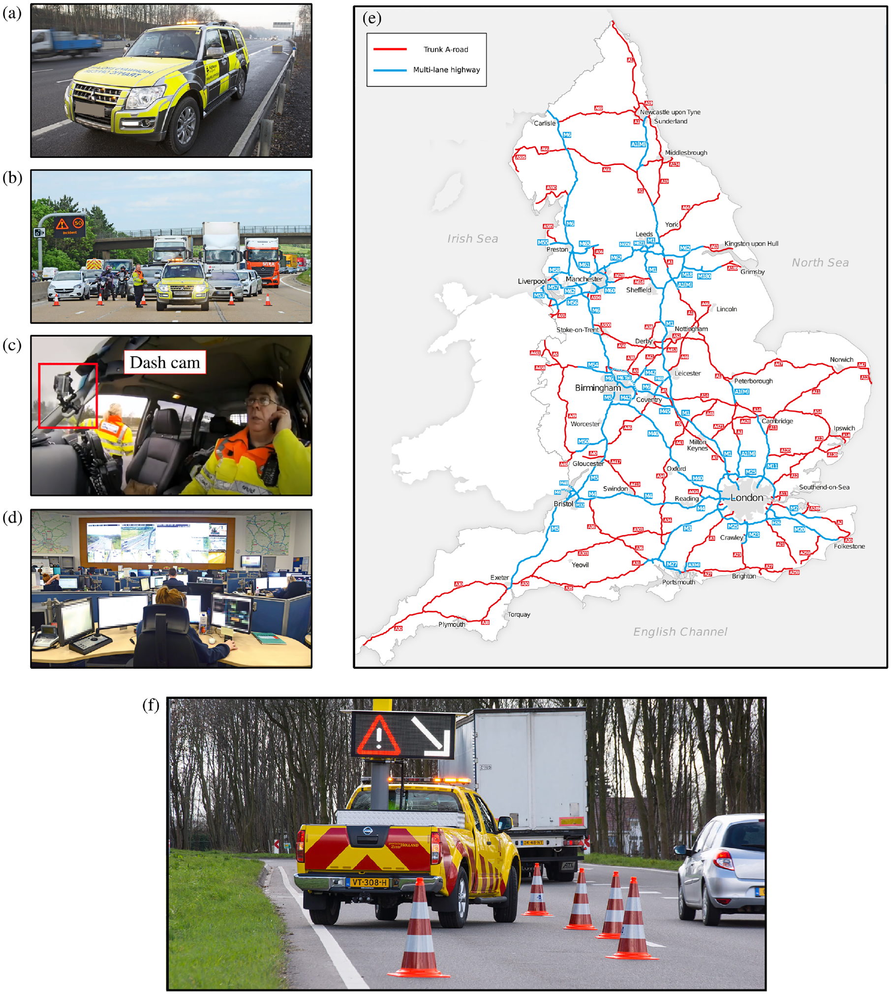
(a) Highways England traffic officers and (f) Weginspecteurs, respectively, patrol along the strategic road network in (e) England, UK and the Dutch highway network. (c) Each traffic officer vehicle is equipped with a dashboard camera, shown in panel. Traffic officers are assigned to (b) attend and manage traffic incidents by (d) regional control center operators.

In the work presented in this paper, we consider a case study of a dedicated TO fleet, who are likely to have relatively relaxed operational constraints compared with their police counterparts. To investigate the feasibility of the proposed TO-based TAM capability, a simulation was developed in which the TOs patrol along the highway and respond to dynamically generated incidents. Two distinct patrol regimes were considered, one that aimed to minimize the fleet’s incident response time and one that aimed to maximize the fleet’s coverage for asset management. By considering the incident response times and coverage achieved by each regime, we aimed to determine the feasibility of deploying the TO fleet for TAM.

Background and Literature Review

Traffic Officer Fleets

TOs are usually formed from a police subunit. For example, the Autobahnpolizei patrol and manage incidents across the German autobahns ( 15 ), the Highway Patrol units (known as state troopers or state police in some states) are deployed on U.S. highways ( 16 ), and the Garda National Roads Policing Bureau ( 17 ) and Polizia Stradale ( 18 ) respectively operate in Ireland and Italy. Alongside managing traffic incidents, such TOs enforce highway laws, for example, apprehend drink drivers and issue speeding fines.

In contrast, dedicated TO fleets, where we see the opportunity, are not as common as those formed from a police subunit; only two (HE and RWS) out of 16 highway agencies across Europe interviewed by Steenbruggen et al. employ a dedicated TO fleet ( 19 ).

While on patrol, HE TOs, shown in Figure 1, either drive along designated patrol routes (typically the busier sections of the SRN) looking for incidents, or they remain stationary in waiting areas. TOs are instructed by operators in regional control centers (RCCs) to respond to incidents via a radio communications system installed in each vehicle.

Although the fleet is not part of the UK emergency services, HE TOs have several extra powers, derived under the Traffic Management Act of 2004 ( 20 ), to quickly and safely clear incidents. For example, an HE TO may stop a vehicle, close highway lanes, and place temporary traffic signs. Furthermore, HE TOs are trained in first aid and CPR (i.e., cardiopulmonary resuscitation) and can provide medical assistance at the roadside ( 21 ). A TO is often first to arrive at an incident and usually takes lead command, unless there is loss of life, when they fall under the command of the emergency services.

Similarly, the Weginspecteurs patrol and respond to traffic incidents across 5,200 km of highway in the Netherlands. Although the Weginspecteur fleet is separate from the police, some TOs in the Netherlands are enrolled as “Extraordinary Investigation Officers” that may compile official reports against drivers for several driving offenses, including ignoring red crosses on variable message signs (VMSs; indicating a lane closure) or driving on the hard shoulder. The Weginspecteur vehicles are fitted with a notable piece of equipment; a large vehicle-mounted VMS to give direct instruction to highway users without relying on a roadside or gantry-mounted VMS.

Vehicle Routing Problems

Designing optimal vehicle routes is a widely studied operations research question known as the vehicle routing problem (VRP). The VRP was first considered by Dantzig and Ramser who developed a method to route a fleet of homogeneous fixed-capacity petrol trucks from a central depot to a series of delivery sites before returning back to the depot ( 22 ). Their method determines a set of shortest paths (one for each truck) along a transportation network defined as a graph of edges (road links) between demand nodes (delivery sites).

There are several VRP variations for specific transportation logistic problems. One popular extension is the VRP with time windows ( 23 ), in which nodes must be serviced within a given time window, to model deliveries to a store that must arrive within its opening hours, for example.

Standard VRPs assume that the demand is static and known before the vehicles begin their routes. However, in most real-world scenarios, the demand is dynamic (hail-and-ride taxi trip requests, for example) and vehicle routes are adjusted during operation (i.e., not at the depot); this extension is known as the dynamic VRP (DVRP).

In a recent review provided by Pillac et al., the DVRP is categorized into two classes; deterministic and stochastic ( 24 ). In the first class of problem, the demand is revealed over time and an optimal solution may only be obtained for the current state. Typically, the deterministic demand problem is solved by periodically invoking a standard VRP (with the demand considered static at that time point) and correspondingly updating the vehicle routes.

The second class of problems consider demand with known statistics (computed from historical data, for example). To solve this stochastic demand problem, an ensemble of hypothetical future demand scenarios is sampled from the known demand distributions, and then solved as a set of static VRPs. Routes that are averaged across the entire ensemble are then chosen.

When assigning a TO to an incident, a control center operator considers the position of the entire fleet and dispatches a TO to minimize the incident response time, that is, the time for the TO to arrive at the incident. Such centralized vehicle dispatching systems (VDSs) are a specialization of the DVRP (with the additional constraint that demand should be serviced as soon as possible) and are found in several demand-driven transportation systems such as hail-and-ride taxis ( 25 ) and emergency repair vehicles ( 26 ).

Both a deterministic and stochastic VDS for a personal rapid transit system are considered by Lees-Miller and Wilson ( 27 ). The deterministic method assigns a vehicle as trips are requested in sequence, whereas the stochastic method moves idle vehicles to stations to service future (sampled) demand. On two test networks the stochastic method achieves up to a 96% reduction in passenger waiting time compared against its deterministic counterpart.

The DVRP becomes complex for large transportation systems, such as highway networks, and rerouting a vehicle multiple times throughout one journey may be unpractical and place a heavy burden on the driver. Furthermore, standard DVRP-based approaches may not be appropriate for vehicles with complicated operational constraints (with time, fuel, or mileage limits, for example) such as a TO or police officer. Instead, complicated transportation problems are often solved through simulations that may incorporate rich application-specific objectives.

The police patrol routing problem (PPRP), concerned with designing patrol routes to minimize the police’s response time to crime while maximally covering a patrol area to deter criminals, is often considered via simulation. The PPRP has a strong analogy with our TO problem—both aim to maximally cover an area (to deter criminals or capture asset data) while minimizing response time (to crime or traffic incidents).

The GAPatrol system developed by Reis et al. is one simulation-based approach to the PPRP ( 28 ). The authors developed a multiagent simulation, based in the Fortaleza area of Brazil, in which a group of criminals randomly try to commit crimes at predetermined targets while avoiding a fleet of police officers. Their genetic algorithm-based method identifies a set of locations for each police vehicle to visit in sequence that minimizes the amount of crime committed in the simulation. A similar simulation is presented by Melo et al., however, in their work they consider various “physical reorganizing” strategies, namely, how police officers drive between crime hot spots ( 29 ). A short-routing strategy, in which police officers drive along the shortest route between hot spots, minimized the amount of crime.

Mobile Sensing for a Secondary Purpose and Maximal Coverage Systems

Mobile systems used for a secondary sensing purpose, such as the system proposed here, are less widely deployed than those designed for a specific application, such as the specialized annual survey vehicles. One example is the pothole patrol system ( 30 ) that uses data from accelerometers installed in taxis across the city of Boston. The primary function of the taxis is not changed—they pick up and drop off passengers as usual. However, by aggregating data collected from the entire fleet, the system is able to automatically detect potholes across the city. Similarly, taxi fleets have also been considered as citywide VANET-based (vehicle ad hoc network) communications and traffic estimation systems ( 31 , 32 ).

The objective of routing agents to maximally cover an area is another widely studied problem. In the pioneering work of Machado et al., the architectures and system considerations for maximal coverage multiagent systems are tested within a simulation ( 33 ). A geographical area is deconstructed into a graph of nodes and edges, and the concept of node “idleness” is introduced, that is, the time between successive node visits from an agent. Several subsequent works have continued to adopt the terminology of site or target idleness ( 34 , 35 ). In research by Machado et al. the agents try to minimize the total node idleness, and thus maximally cover the graph ( 33 ). Various routing strategies, including a greedy algorithm in which each agent only considers their immediately neighboring nodes, and more complex strategies in which agents consider a larger neighborhood of nodes are tested. Various communication styles are also tested, including decentralized methods by which agents leave environmental “flags” at the nodes for other agents to sense, centralized communication with a control center, and communication via agent interaction. Our problem differs in that the TOs consider the idleness of the highway sections, rather than nodes. However, many of the topics covered are relevant considerations when deploying our TOs for TAM.

Data Sources and Preparation

We will now focus our study into the HE TO fleet on the SRN in England, for which there is comprehensive data that we will now describe. See Table 1.

Table 1.

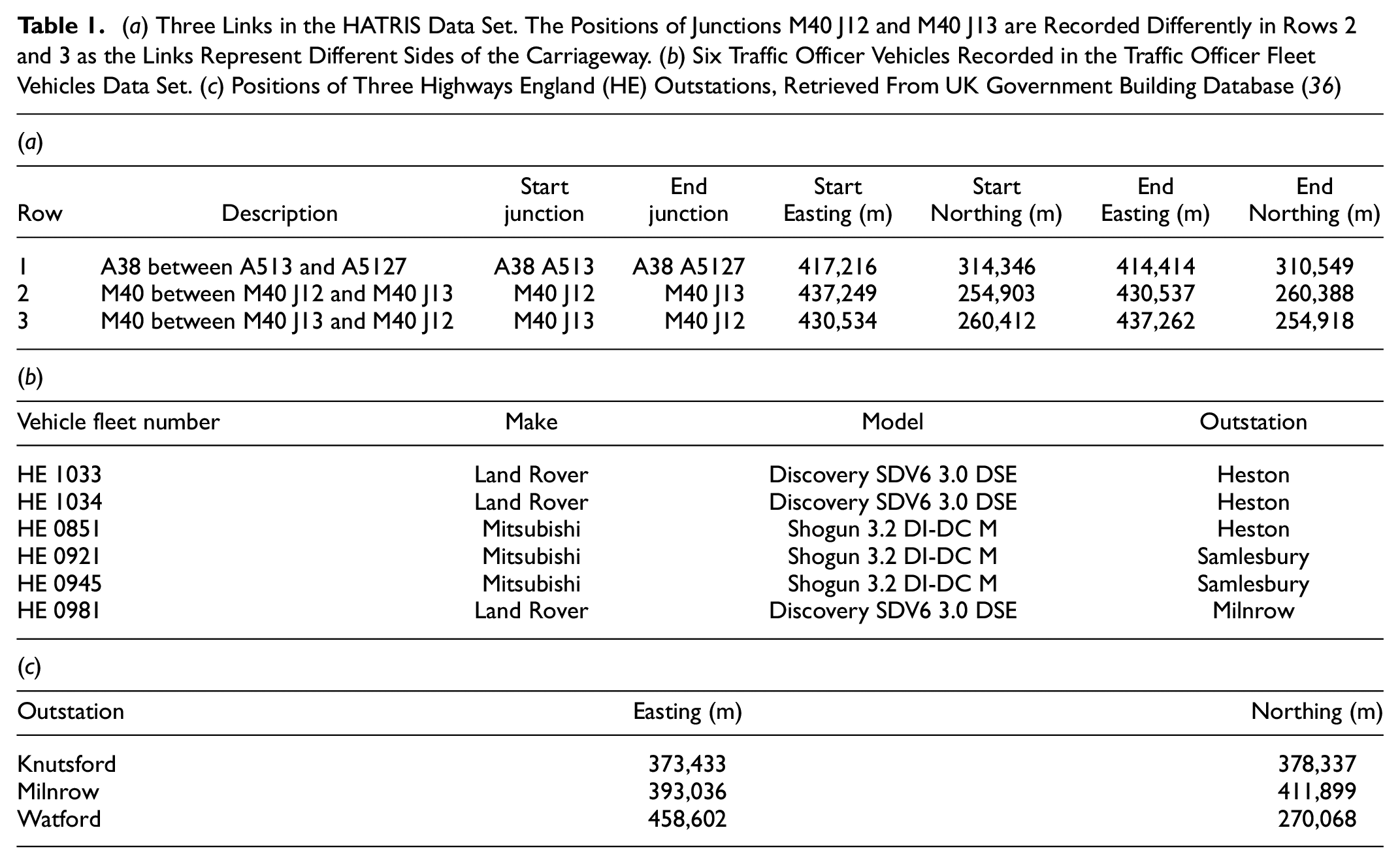
(a) Three Links in the HATRIS Data Set. The Positions of Junctions M40 J12 and M40 J13 are Recorded Differently in Rows 2 and 3 as the Links Represent Different Sides of the Carriageway. (b) Six Traffic Officer Vehicles Recorded in the Traffic Officer Fleet Vehicles Data Set. (c) Positions of Three Highways England (HE) Outstations, Retrieved From UK Government Building Database ( 36 )

(a)
Row	Description	Start junction	End junction	Start Easting (m)	Start Northing (m)	End Easting (m)	End Northing (m)
1	A38 between A513 and A5127	A38 A513	A38 A5127	417,216	314,346	414,414	310,549
2	M40 between M40 J12 and M40 J13	M40 J12	M40 J13	437,249	254,903	430,537	260,388
3	M40 between M40 J13 and M40 J12	M40 J13	M40 J12	430,534	260,412	437,262	254,918

(b)
Vehicle fleet number	Make	Model	Outstation
HE 1033	Land Rover	Discovery SDV6 3.0 DSE	Heston
HE 1034	Land Rover	Discovery SDV6 3.0 DSE	Heston
HE 0851	Mitsubishi	Shogun 3.2 DI-DC M	Heston
HE 0921	Mitsubishi	Shogun 3.2 DI-DC M	Samlesbury
HE 0945	Mitsubishi	Shogun 3.2 DI-DC M	Samlesbury
HE 0981	Land Rover	Discovery SDV6 3.0 DSE	Milnrow

(c)
Outstation	Easting (m)	Northing (m)
Knutsford	373,433	378,337
Milnrow	393,036	411,899
Watford	458,602	270,068

Traffic Officers

Each vehicle in the HE TO fleet is recorded in the traffic officer fleet vehicles (TOFV) data set published by HE in 2018 ( 37 ). For each vehicle, the TOFV data set records its vehicle fleet identifier, make, and model, and the outstation from which the vehicle begins and ends its patrol. In total, the TOFV data set consists of 234 vehicles that patrol from 32 outstations across the SRN.

Outstations

The name of each of the 32 TO outstations across the SRN is listed on the HE website ( 38 ). To determine the position of each outstation, their addresses were obtained via an online UK government building database ( 36 ) and converted to an Easting–Northing coordinate ( 39 ) to the nearest meter.

Strategic Road Network

The SRN is represented by the Highways Agency (HE’s name before 2014) traffic information service (HATRIS) links ( 40 ) that describe the junction-to-junction sections of the SRN. The links were initially used to report traffic flows between each junction until the service was upgraded in 2016 to provide live traffic information along shorter interjunction highway sections ( 41 ).

For each link, its highway name (e.g., M6) and the start and end junction name (e.g., J1) and position as an Easting–Northing coordinate to the nearest meter are recorded. Junctions along major highways are named by their junction number (e.g., M6 J1), however junctions along smaller highways are defined by the connecting road at the junction. For example, the A38 connects to the A515 (which is not part of the SRN) at Junction A38 A515. In total, 2,510 links are recorded.

Graphical Highway Network Model

The recorded positions for each HATRIS junction with the same name were collected and their pairwise distances computed. Those pairs for which the distance was greater than 4 km were then flagged for manual inspection and cleaning, since it seemed likely that they were in fact different junctions that happened to have the same name (for example, because pairs of “A” roads might happen to meet at several different places).

An abstract graphical highway model ( 42 ) of the SRN was then constructed from the cleaned HATRIS links and junctions. The junctions provide the graph’s nodes and each HATRIS link represents a directed edge between those nodes. The driven distance for each edge was then modeled crudely by the straight-line distance between its nodes, based on their coordinates. An improved edge distance might be obtained via a mapping service (e.g., OpenStreetMap [43]) in which distances along curved highway sections may be computed. However, we have left such refinement of the graphical highway network model for future work.

Unfortunately, the HATRIS data do not provide unambiguous junction coordinates: see Table 1a, Rows 2 and 3, which represent the opposing directions of the same dual carriageway section. Because of the lateral physical scale, different coordinates are recorded for the junction position for each side of the carriageway. Our approach was thus simply to take the average of all of the coordinates provided for a given junction.

The resulting graph (Figure 2) consists of 1,108 nodes and 2,376 directed edges, with a total length of 13,048 km. HE report a total network length of 13,760 km ( 44 ); the small difference can be accounted for by our neglection of link curvature.

Figure 2.

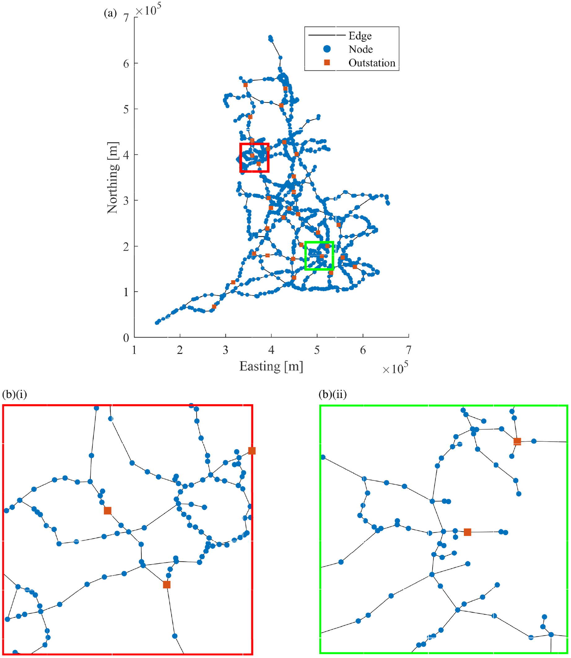
(a) The strategic road network (SRN) graph constructed from the HATRIS links and (b) two zoomed areas. For illustration purposes, each edge in this figure represents two directed edges (one for each direction of travel). The nodes closest to each outstation are depicted with orange squares.

Concepts of Operation

We now proceed to describe and simulate the proposed operational mode of the TOs. We will use the term FTO (future traffic officer) to distinguish between the new concepts of operation that we propose, and the current real-world practice.

Multilane highways usually have a central reservation and TOs can thus only reroute at junctions. Thus, we describe their operation in relation to a node-to-node routing methodology on the graphical model of the highway developed in the previous section. Note that as each junction is collapsed onto a single node, neither its size nor drive-through structure is modeled (these generalizations remain for future work). As an FTO reaches a node, it was assumed that they may instantaneously choose which of the connecting edges to patrol (and capture asset data) along next. However, junctions are small compared with the length of highway between them, and maximizing the fleet’s coverage on the SRN (for asset management) can be well approximated by considering the edge coverage only.

On reaching a node, we supposed that each FTO would make one of the following decisions:

Continue on the same highway;

Join a new highway;

Turn around and drive along the same highway in the opposite direction; or potentially,

Stop for a rest period, albeit remaining available during this time for incident response.

The key idea was that different patrol regimes (that prioritize either incident response or asset management) would influence this routing decision.

In notation: the state of FTO, $k$ , is fully described by the node it is driving to, and the time it will arrive (and simultaneously depart from) there, respectively denoted by $n [k]$ and $a [k]$ . The edge from node $i$ to $j$ has intervisit time (idleness), $v (i, j)$ , and driven distance, $d (i, j)$ (recall that this is modeled by the node-to-node straight-line distance). The distance matrix, $D$ describes the pairwise node shortest path length, and the trip time matrix is given by $T = D / s$ , where we suppose that $s = 100$ km/h is the constant FTO speed.

The real-world TO, who may encounter congested traffic conditions, is unlikely to drive at a constant speed throughout their patrol. However, in the absence of intrajunction, granular (e.g., collected every minute) traffic speed data across the entire SRN, we assumed a constant TO speed in this first work. Moreover, none of the patrol regimes described in the following section depend directly on the TO’s speed, which may thus be viewed as a separate module of the simulation to be improved in future versions of the simulator.

Traffic Officer Patrol Regimes

We analyzed three patrol regimes:

Response (R1),

Coverage (R2), or

Random (R3).

The idea is that R1 aims to minimize the fleet’s collective incident response time, whereas R2 aims to maximize the fleet’s coverage for asset management. In R3, FTOs select their next edge at random, and this will act as a base case, which R1 and R2 must outperform.

Under R1 (Figure 3a), FTO $k$ considers a neighborhood $N$ of close nodes, within a driven distance $δ_{n}$ of node $n [k]$ , and a set $F$ of close FTOs, within a driven distance $δ_{f}$ of node $n [k]$ . The idea is that FTOs continuously attempt to collectively minimize their drive time to any node within their near neighborhood, in case an incident should occur there in the near future. This is achieved in a distributed way by each FTO selecting their next edge, $e^{*}$ , according to

e^{*} = \underset{e}{\arg \min} \sum_{n \in N} {\bar{r}}_{n},

(1)

where

{\bar{r}}_{n} = w_{n} min ({r_{e} (k, n) \cap r (f, n) : f \in F})

(2)

is the weighted minimum incident response time (WMIRT), and

r_{e} (k, n) = T (n [k], n_{e}) + T (n_{e}, n)

(3)

where $n_{e}$ denotes the destination node of edge $e$ , is the response time of FTO $k$ to node $n$ if it chooses to patrol along edge $e$ . The response time of FTO $f$ to node $n$ is denoted by $r (f, n)$ . Note $w_{n}$ is a weight attached to node $n$ that models its relative frequency in experiencing incidents.

Figure 3.

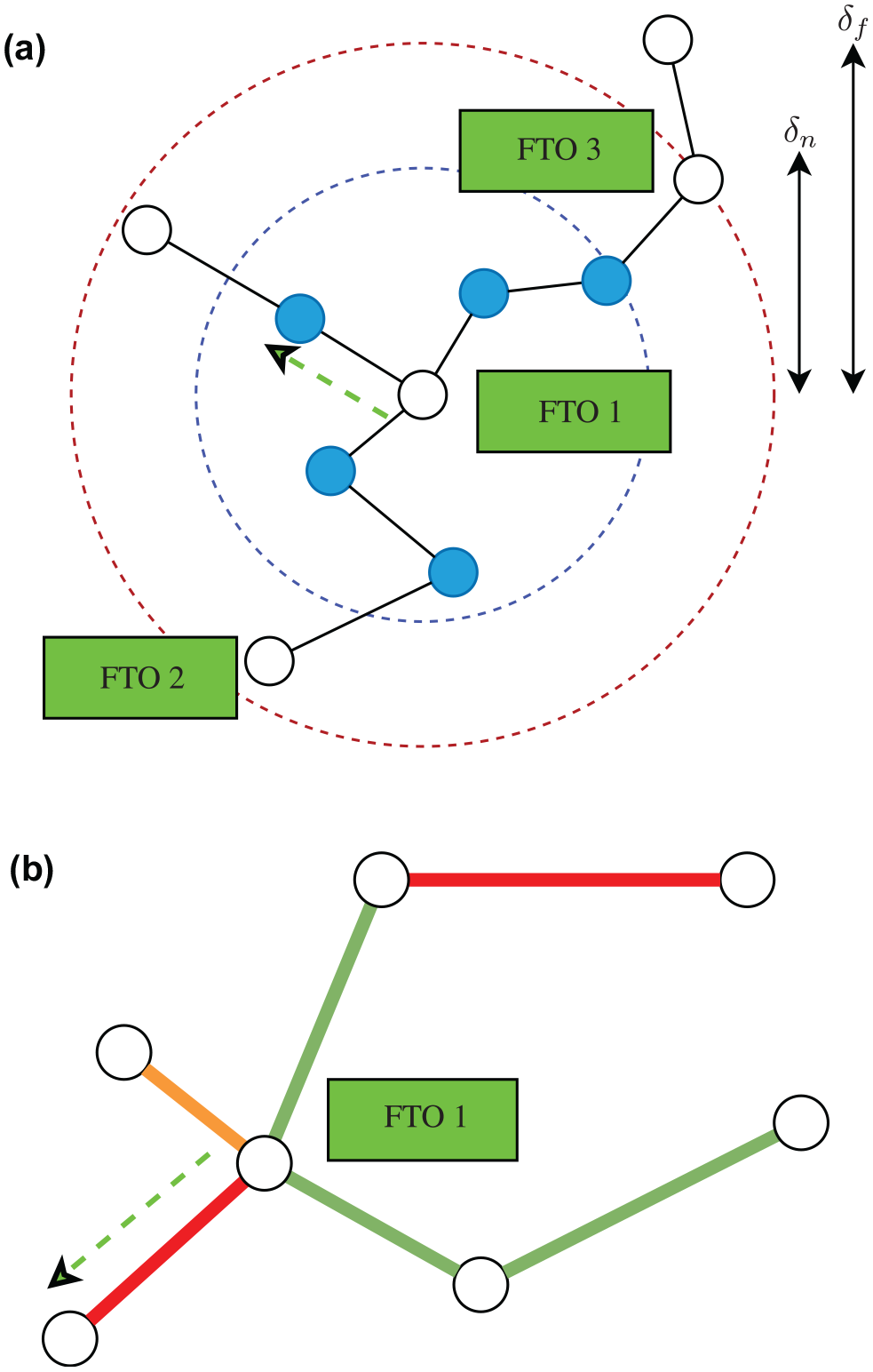
(a) Under R1 future traffic officer (FTO) 1 selects the edge to minimize the total weighted minimum response time to a nearby node neighborhood (blue), from either itself, FTO 2, or FTO 3. (b) Under R2 FTO 1 selects the edge with the largest intervisit time (red).

In contrast, in R2 (see Figure 3b), FTO $k$ selects the connecting edge with the largest intervisit time, that is,

e^{*} = \underset{e}{\arg \max} [v (n [k], n_{e})] .

(4)

In R3, the edge, $e^{*}$ , is chosen uniformly at random from the allowed options. Once FTO $k$ has chosen which edge $e^{*}$ to patrol along, their state is updated according to $n [k] = n_{e^{*}}$ and $a [k] = a [k] + T (n [k], n_{e^{*}})$ , and the intervisit of the edge is updated such that $v (n [k], n_{e^{*}}) = 0$ minutes.

Incident Response Mechanism

From time to time, incidents will occur and the FTOs will break off from their usual patrolling pattern. We suppose that the Bell and Wong Nearest Neighbor (BWNN) heuristic ( 25 ) is employed to assign the nearest FTO to the incident and thus minimize the response time. In notation, given an incident at time, $t$ , along an edge from node $i$ to node $j$ , BWNN assigns a single FTO, $k^{*}$ , by

k^{*} = \arg min_{k} [r (k, i)] .

(5)

Here,

r (k, i) = max (0, a [k] - t) + T (n [k], i) + t_{inc}^{i}

(6)

is the time for FTO $k$ to drive to node $i$ , plus the time taken to drive from node $i$ along the edge to the incident, denoted $t_{inc}^{i}$ . Correspondingly, $t_{inc}^{j}$ denotes the time to drive from the incident to the edge’s destination node.

We suppose that asset monitoring continues while the selected FTO drives to the incident, and thus the intervisit times of the edges along the shortest path from node $n [k^{*}]$ to node $i$ , and the edge from node $i$ to node $j$ , are set to zero as the FTO passes them. Moreover, we suppose that the assigned FTO is unavailable to respond to further incidents before clearing its current assignment. (Of course, one might consider much more sophisticated operations in which, for example, a multivehicle collision requires that multiple FTOs are deployed and taken from other less urgent assignments—this is beyond our current scope.)

Once the incident is cleared, we assume that the FTO, $k^{*}$ , drives to node $j$ , and thus $n [k^{*}] = j$ and

a [k^{*}] = t + r (k^{*}, i) + t_{TTC} + t_{inc}^{j},

(7)

and then resumes their usual patrolling regime. Here, $t_{TTC}$ and here models the incident’s time-to-clear (TTC) ( 45 ).

Simulation Methodology

Initialization and Time Stepping

At the beginning of the simulation, the intervisit time of each edge is set to 0 min; essentially, assets across the entire highway network begin in a perfect state (as if they have just been visited) and now require monitoring throughout the new patrol. Of course, in reality, each asset’s condition will depend on several factors, such as its material properties and age, for example. However, the initial edge start intervisit times proposed here (i.e., 0 min) provide a consistent initialization to run and compare multiple simulations (under each patrol regime) against.

Inspired by the day–night patrol pattern employed by HE and RWS ( 11 , 46 ), each simulated FTO begins a 12-h patrol shift at $t = 0$ min from the node closest to its outstation. Each FTO must return to this node by the end of the shift and is thus constrained by an operational radius that shrinks throughout the simulation. However, we allow an FTO to leave their operational area to respond to an incident.

While on patrol, HE TOs drive for half of their shift and rest at junctions or parking areas for the other half (HE, personal communication). To model this, our simulated FTOs repeatedly drive for 1 h and then rest at a node for 1 h. The first rest time of each FTO is randomly assigned within the first hour of the simulation to ensure that the entire FTO fleet is not resting at the same time. All simulated FTOs patrol under the same regime throughout the 12-h patrol.

A simulation time step, $Δ t = 1$ min, is chosen and in each time step the update rules are applied to each simulated FTO in sequence. At time step $m$ , provided $m Δ t < a [k]$ , FTO $k$ will proceed along its current edge, provided it is not called to an incident. The node decision logic is then applied when $m Δ t \geq a [k]$ , and the excess time, $m Δ t - a [k]$ is subtracted from the arrival time at its next node.

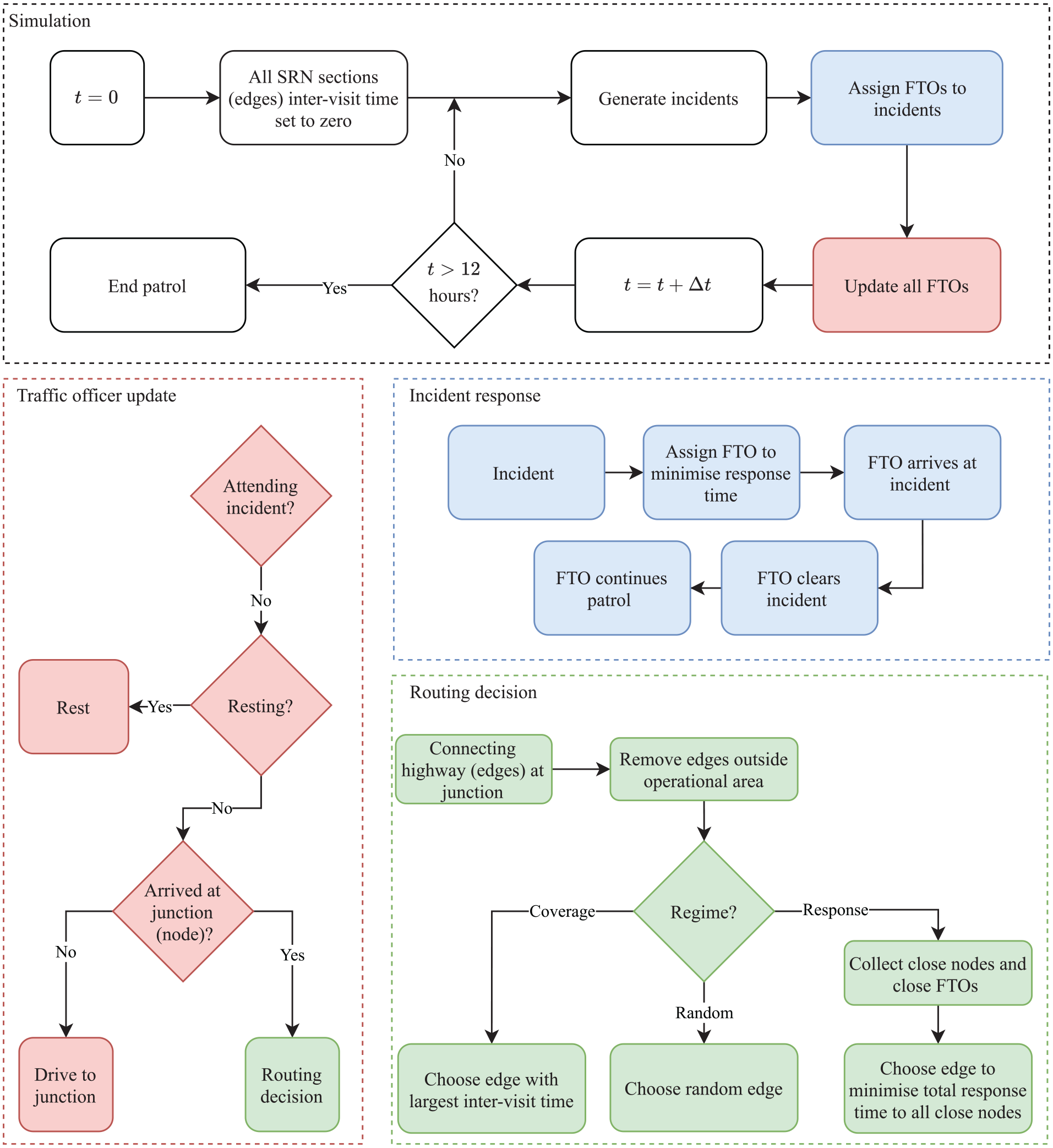
We experimented with varying values of $Δ t$ , however the simulation was found to be robust (i.e., overall, the incident response times and edge intervisit times were unchanged) when the time step was refined. A top-level simulation architecture is provided in Figure 4.

Figure 4.

Simulation architecture. The future traffic officers (FTOs) patrol for a 12-h shift and respond to incidents as they are generated (blue). On reaching a node, provided they are not resting, each FTO chooses which edge to patrol along next via the routing decision process (green), which is influenced by the FTO’s patrol regime.

Incident Model

Vehicle incidents on highways are often modeled by a Poisson process in space and time ( 47 – 49 ) that models each incident as an independent event. Furthermore, the rate at which a given edge suffers incidents is proportional to its length ( 49 , 50 ).

In any time step, the probability of there being one event on an edge, from node $i$ to node $j$ , is approximately $λ d (i, j) Δ t$ . Since this scales with small $Δ t$ , we took the usual approach and supposed that the probability of more than one event on a given edge in one time step would be zero. Each incident was randomly positioned along the edge and was given HE’s target TTC of t_TTC = 60 min ( 51 ). Again, in the absence of TTC distribution data across the SRN (previous works have calibrated TTC distributions with historical incident data across highway networks in Michigan and Los Angeles [52, 53], for example), we assumed a constant TTC (rather than sampling from a known distribution) in this initial model and refinements remain for future work.

In 2015, HE TOs attended 215,568 incidents, equal to 0.41 incidents per minute ( 54 ). Dividing this quantity by the total length of the SRN yields an incident rate $λ = 3.14 \times 10^{- 5}$ incidents per kilometer per minute.

Determination of Response Regime Parameters and Node Weightings

Under R1, each FTO considers the position of other nearby FTOs, to minimize the total WMIRT to a nearby node neighborhood (see Equations 1 and 2). As the number of incidents on an edge is proportional to its driven distance, and each incident is randomly positioned along the edge, we modeled the weight, $w_{n}$ , of node $n$ by the total driven distance of its outgoing edges.

FTOs patrolling under R1 emerge into a kind of formation in which each FTO patrols close to a response node; namely, a node from which the total WMIRT to all nodes in the neighborhood is minimized.

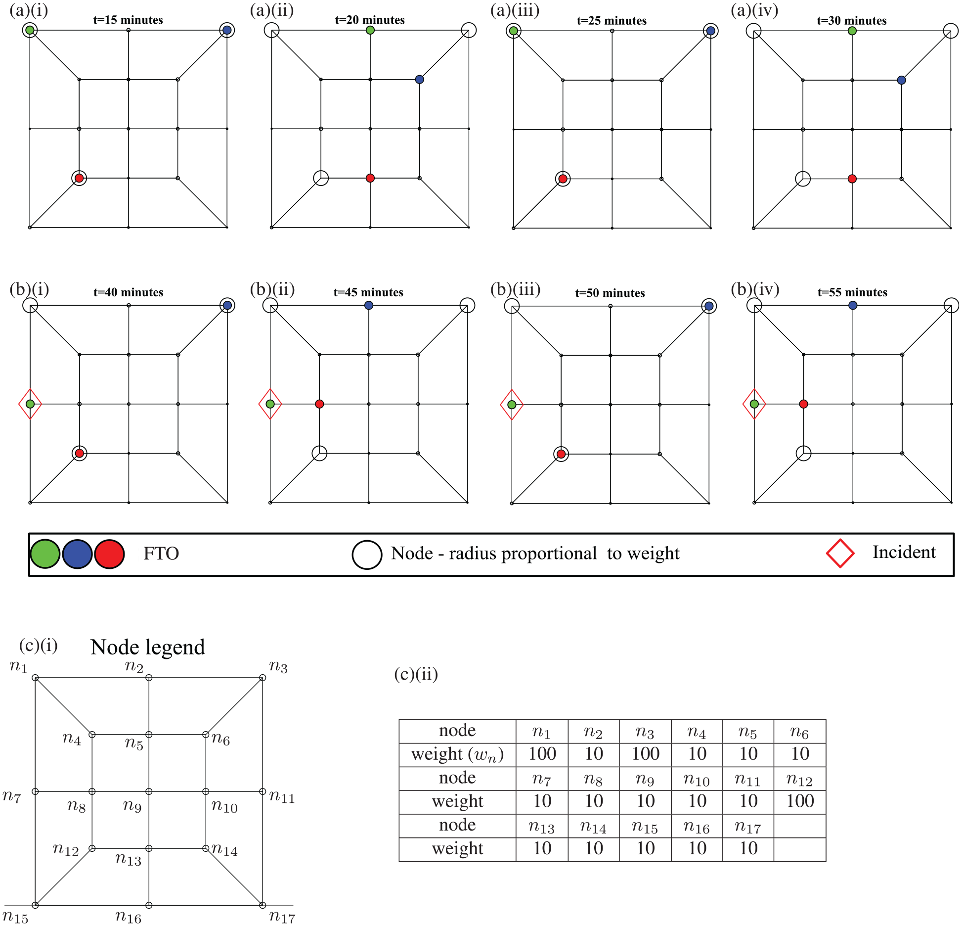
When an FTO is assigned to an incident, they leave their response node and break the formation, then, the remaining unassigned FTOs emerge into a new formation. This reformation process is demonstrated in Figure 5 with a small fleet of three FTOs on a gridlike test graph, with 17 nodes and 28 edges each with length 10 km. For this test case, $δ_{n}$ is set such that each FTO’s node neighborhood is the entire graph, and $δ_{f}$ is set such that each FTO may always communicate with the other two.

Figure 5.

Three future traffic officers (FTOs) on a test network under R1. Nodes $n_{1}$ , $n_{3}$ , and $n_{12}$ have weight 100, whereas the rest have weight 10 (see node legend and weights in the [c] panels). At the beginning of their patrol (a) the FTOs emerge into an initial formation. (b) At t = 40 min the green FTO responds to an incident, and the two unassigned FTOs arrange themselves into a new formation.

Three nodes in the test graph were given an increased weight of 100 whereas all other nodes had weight 10, and thus, the FTOs weight the minimum response time to these three nodes more heavily. Note that in this test case scenario, the weights were assigned independently of the edge length.

Intuitively, optimal R1 parameters will distribute the FTOs to response nodes across the SRN graph, so that an FTO may respond quickly to any incident. For the SRN graph considered in this paper, parameter values of δ_n = 80 km and δ_f = 80 kmwere found to distribute the FTOs (into desirable emergent formations) across the entire graph.

Simulation Metrics and Analysis

The incident response times and edge intervisit times were compared over an ensemble of 50 simulations under R1, R2, and R3 (150 in total). Four patrol routes from the ensemble are illustrated in Figure 6. Specifically, at simulation time, $t$ , we considered the ensemble-average incident response time (AIRT) and edge intervisit time (AIVT), respectively computed by

AIRT (t) = \frac{1}{| N_{inc} |} \sum_{n \in N_{inc}} r (k^{*}, n)

(8)

and

AIVT (t) = \frac{1}{| E |} \sum_{(i, j) \in E} v (i, j) .

(9)

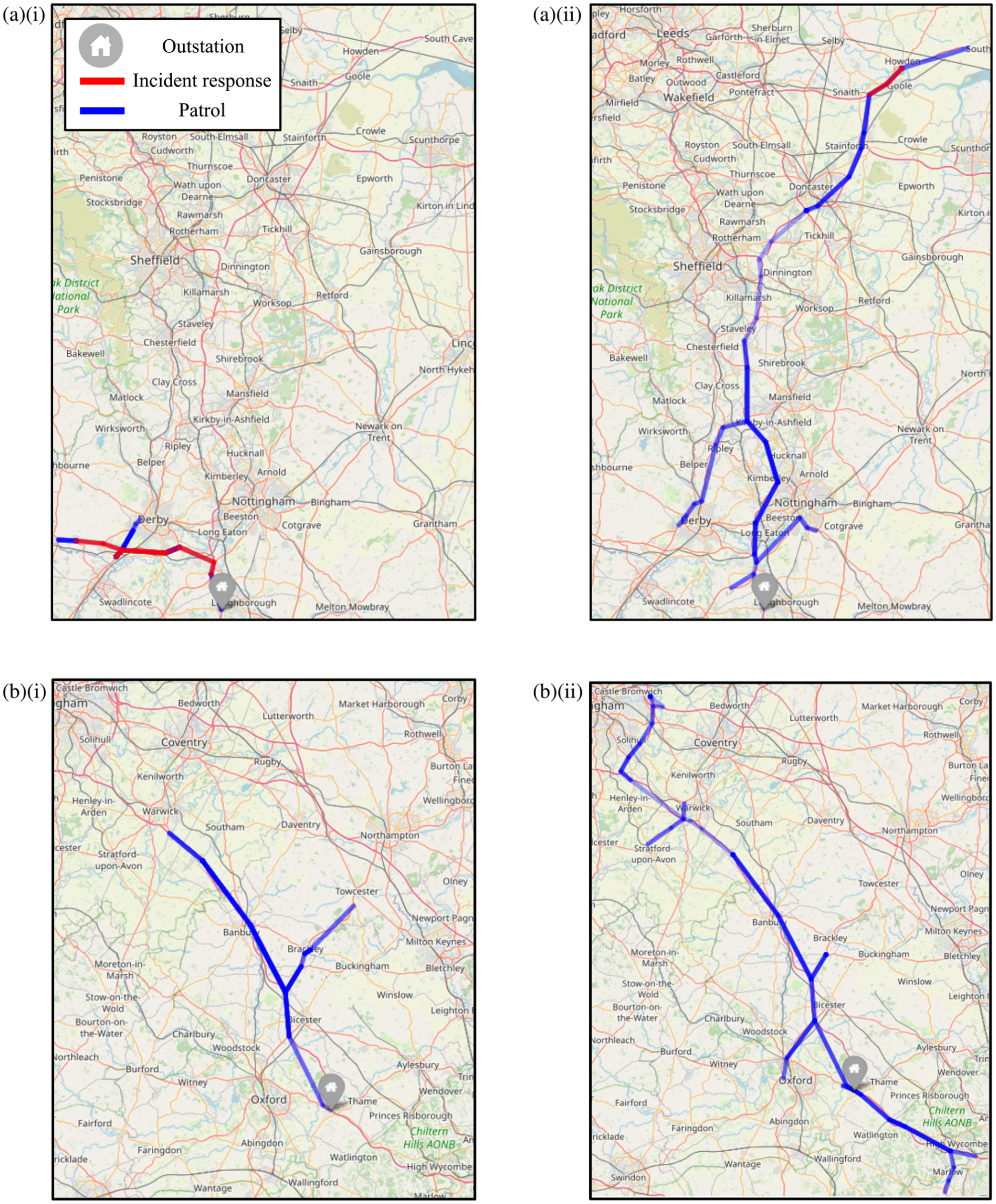
Here, N_inc denotes the start node of those edges where an incident occurs at time t (and is attended by FTO $k^{*}$ ), and nodes $i$ and $j$ respectively denote the start and end nodes of each edge in the set of SRN graph edges E.

Figure 6.

Future traffic officer (FTO) patrol routes from the (a) Shepshed and (b) Milton Common outstations. The (i) and (ii) panels respectively correspond to patrols under R1 and R2. Blue sections of highway indicate the FTO’s usual patrolling pattern, whereas red indicates incident response: a darker color illustrates where the FTO has regularly patrolled. All panels were generated via the OpenStreetMap mapping service ( 43 ).

AIVT is a suitable metric to consider for those assets that require immediate management (and thus continuous monitoring), such as debris on the highway surface. However, a daily asset data capture was specified by HE as a suitable monitoring frequency for assets whose condition might rapidly change but do not require immediate management, such as a broken streetlight for example (HE, personal communication). Therefore, in addition to the AIVT, we also computed the ensemble-average percentage of edges that were visited at least once by an FTO (APV) during the 12-h patrol. Specifically, at simulation time $t$ , the APV is computed by

APV (t) = 100 \times \frac{1}{| E |} \sum_{(i, j) \in E} V (i, j),

(10)

where

V (i, j) = {\begin{matrix} 1 & if v (i, j) < t, \\ 0 & otherwise . \end{matrix}

(11)

Simulation Run-In and Return Period

The ensemble AIVT and AIRT at each simulation time step are shown in Figure 7. The simulations exhibited a run-in period during the first 150 min of the patrol as the FTOs departed from their outstations and patrolled on a small proportion of the SRN graph. The FTOs returned to their outstations during a return period (t > 650 min). Consequently, under R2, the AIVT increased as each FTO was restricted by their operational radius. On the other hand, under R1, the AIVT decreased as the FTOs broke their emergent formations. The AIRT increased under all regimes during both the run-in and return periods.

Figure 7.

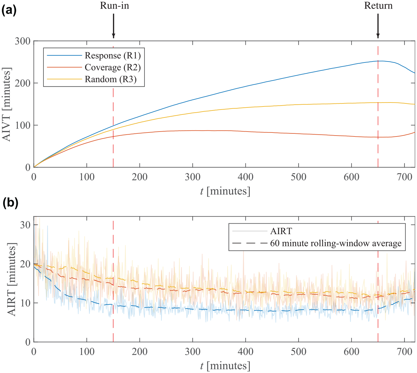
(a) Average edge intervisit time (AIVT) and (b) average incident response time (AIRT) along with a 60 min rolling-window average under each regime. The simulations exhibit a run-in period (t < 150 min) and a return period (t > 650 min) as the future traffic officers (FTOs) leave and return to their outstations.

To assess the regimes while avoiding the impact of the run-in and return periods, we computed and compared the time-averaged AIRT (TAIRT) and AIVT (TAIVT) in the time window $150 \leq t_{w} \leq 650$ min, such that,

TAIRT = \frac{1}{| t_{w} |} \sum_{t_{w}} AIRT (t_{w})

(12)

and

TAIVT = \frac{1}{| t_{w} |} \sum_{t_{w}} AIVT (t_{w}) .

(13)

Here, $| t_{w} |$ denotes the number of time steps in the time window (500 for $Δ t = 1$ min). Similarly, we considered the APV at the end of the time window (APVW),

APVW = APV (650 \min);

(14)

essentially, this is the percentage of edges visited by at least one FTO before the return period.

Simulation Results

The TAIRT, TAIVT, and APVW under each regime are given in Table 2. Overall, R2 decreased the TAIVT by 106.46 min and the APVW by 15% compared with R1, whereas the TAIRT only increased by 3.93 min. The ensemble distributions for the incident response time, and the edge intervisit time at t = 650 min are provided in Figure 8.

Table 2.

TAIRT, TAIVT, and APVW Achieved by an FTO Fleet of 234 Vehicles. The Difference Row Shows the Difference Between R2 and R1. Overall, R2 Reduces the TAIVT by 106.46 Min and Increases the APV by 15%, Whereas, the TAIRT is Only Increased by 3.93 Min

Regime	TAIRT (min)	TAIVT (min)	APVW ( $%$ )
Response (R1)	8.52	186.74	83
Coverage (R2)	12.45	80.28	98
Difference	3.93	−106.46	15
Random (R3)	13.41	135.16	93

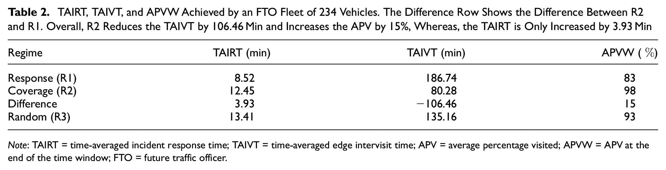
Note: TAIRT = time-averaged incident response time; TAIVT = time-averaged edge intervisit time; APV = average percentage visited; APVW = APV at the end of the time window; FTO = future traffic officer.

Figure 8.

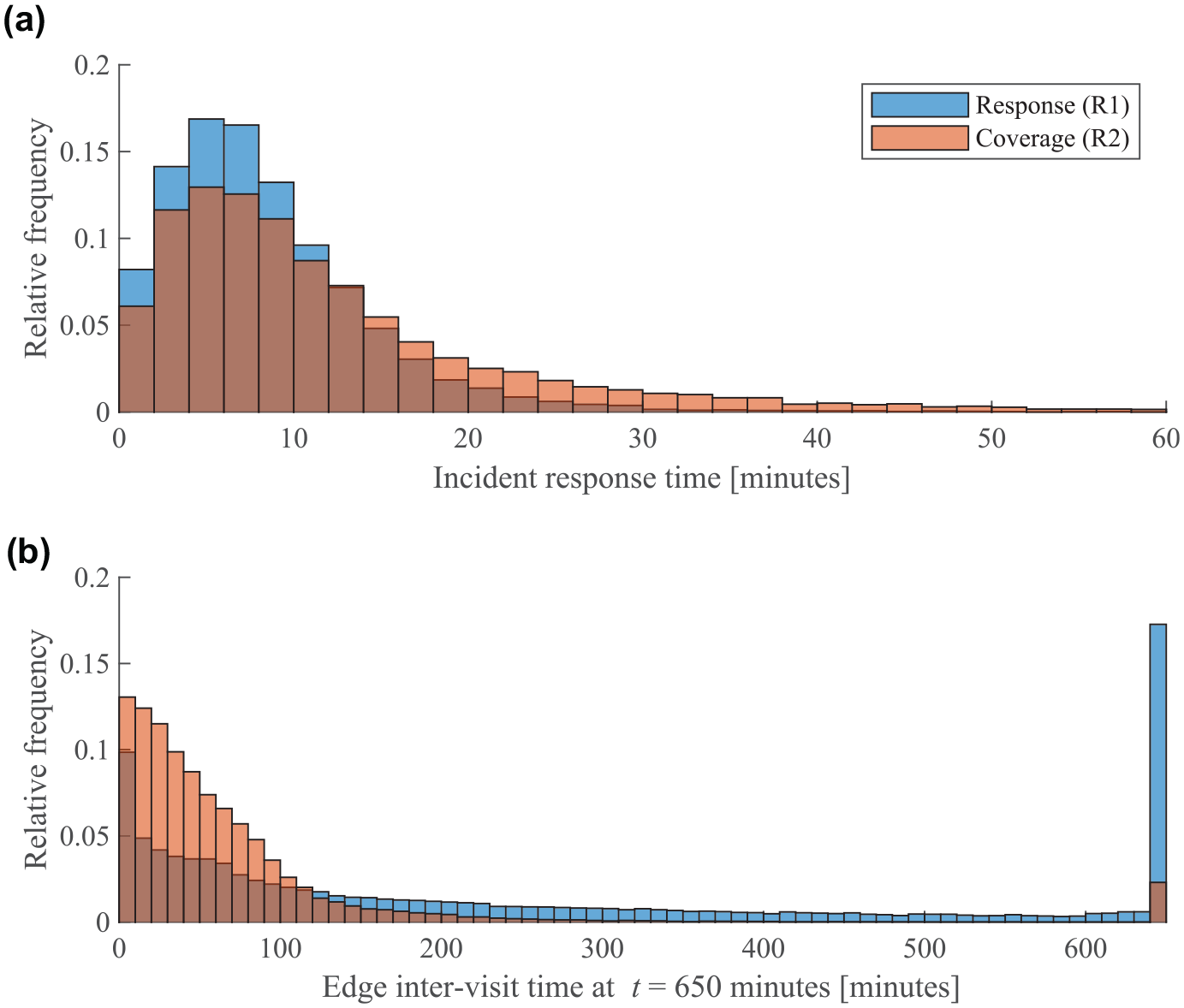
(a) Ensemble incident response times and (b) edge intervisit time distributions at t = 650 min under R1 and R2. The incident response mechanism (Bell and Wong nearest neighbor [BWNN]) is identical under both regimes and thus the response time distributions have a similar profile. Under R1, the future traffic officers (FTOs) frequently visit edges close to response nodes, thus, there are an anomalously large number of intervisit times from 0 to 10 min, and a large proportion of edges that are not visited at all.

The incident response mechanism (BWNN) was identical under all patrol regimes and thus the incident response time distributions had a similar profile for both R1 and R2. In contrast, R1’s intervisit time distribution exhibited a relatively heavy tail compared with R2, and 17% of edges were not visited at all during the patrol. In addition, an anomalously large number of intervisit times from 0 to 10 min were exhibited under R1, because those edges connecting to response nodes were visited more regularly.

Varying Fleet Sizes

Figure 9 shows the TAIRT, TAIVT, and APVW achieved by each regime for varying fleet sizes (averaged across 30 simulations per fleet size). When the fleet size was small, the number of incidents overwhelmed the fleet and a queue of incidents for each FTO to attend built. Consequently, the FTO patrol was identical under all regimes; each FTO attended and cleared an incident, and then attended the next and so on. As a result, all regimes achieved an asymptotically large TAIRT, and small TAIVT and APVW.

Figure 9.

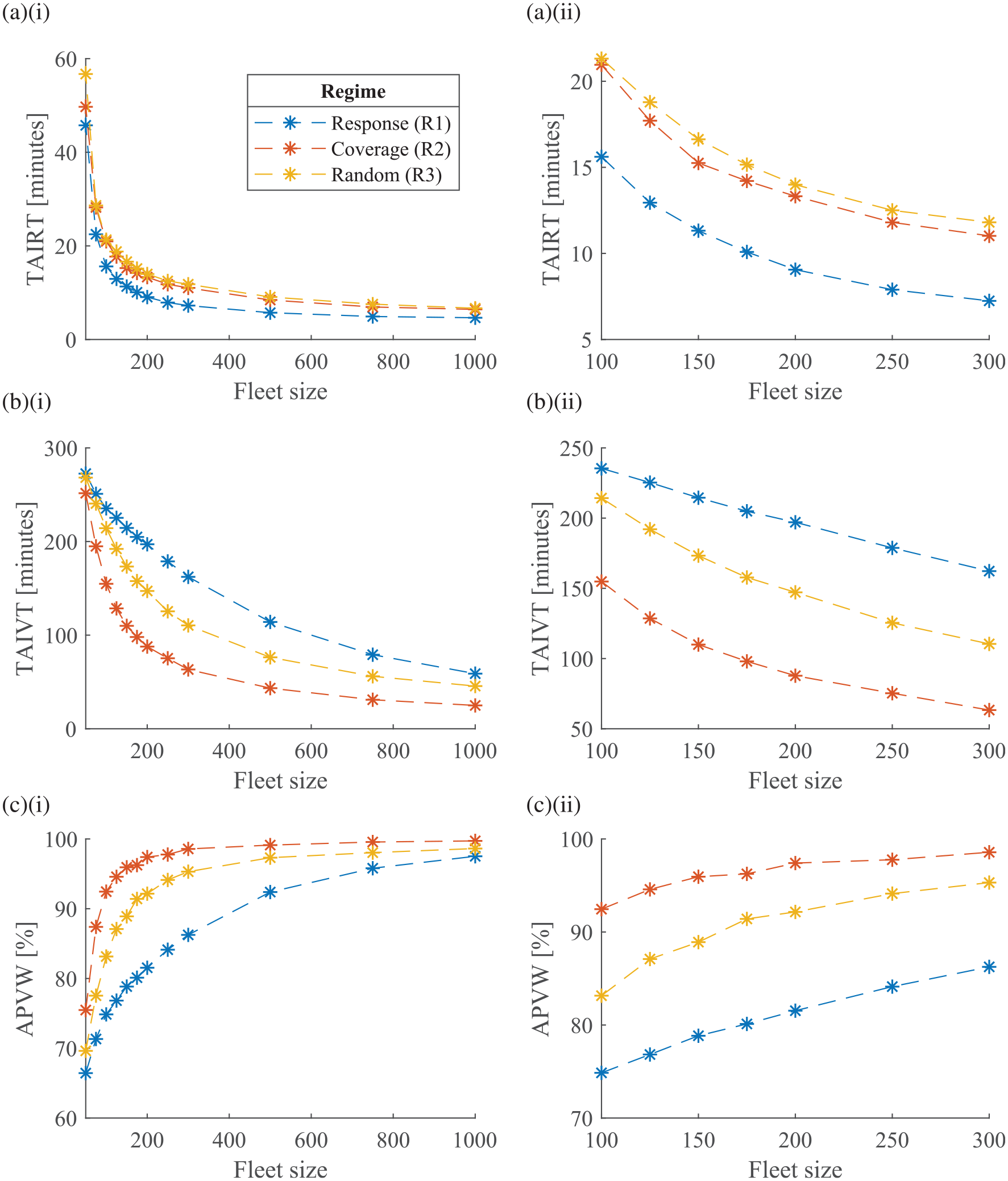
Panels (a) to (c) respectively show the TAIRT, TAIVT, and APVW for varying fleet sizes. The (i) panels show each metric across a wide range of fleet sizes whereas the (ii) panels are cropped to show more realistic fleet sizes.

At the other extreme, for large fleet sizes, the number of FTOs approximated the number of nodes in the graph (1,108). In this case, the fleet was equally well distributed under either regime and the metrics tended toward an asymptotic value. The key result shown in Table 2 is reproduced for all realistic fleet sizes—the FTO fleet could be deployed to efficiently collect asset data across the SRN, while only increasing the fleet’s incident response time by a few minutes.

Discussion

The TAIRT achieved by R2 was only a 0.96-min improvement on R3 (random)—this result is unsurprising as neither regime tried to position the fleet for fast incident response. However, R2 still achieved a TAIRT well under HE’s current AIRT of 17 min, and only 2.45 min over their target response time of 10 min ( 55 ).

R1 reduced the TAIRT by 3.93 min (compared against R2) but only minimized the intervisit times of edges close to response nodes or along the shortest path to an incident. Consequently, the TAIVT was significantly larger under R1, compared with R2 and R3. Furthermore, on average, 17% of edges were not visited at all under R1, whereas only 2% of edges were not visited under R2. The key result, that R2 significantly reduced the TAIVT and APVW but only increased the TAIRT by a few minutes, was reproduced for all realistic fleet sizes (see Figure 9), and thus, our simulations showed the potential to use TO fleets for asset management.

In this work, we have considered a base-case regime in which each FTO chooses an edge at random (R3). Of course, there are other regimes that may result in longer incident response times and reduced coverage—every FTO remaining at their outstation, for example. However, R3 employed the same node-to-node routing methodology as that in R1 and R2, and thus seems an appropriate base case.

The increase in incident response times (IRTs) versus the increase in network coverage (for TAM) under R2 requires careful consideration from agency decision makers who wish to employ our proposed concepts of operation—some agencies may not tolerate any increase in IRTs. However, a hybrid approach, in which TO fleets patrol under a mixture of regimes, might provide a more flexible operational framework with which to consider the IRT–network coverage tradeoff.

Figure 10 shows the TAIRT and TAIVT achieved by the HE TO fleet (224 vehicles) when patrolling under a mixture of R1 and R2: the bottom axis indicates the percentage of TOs patrolling under R2 (PFR2, the remaining TOs patrol under R1). Each PFR2 result was averaged over 20 simulations, and the TOs patrolling under R2 were randomly assigned for each new patrol. The results showed that, for example, PFR2 = 30% decreased the TAIVT by around 80 min (compared with PFR2 = 0%), whereas the TAIRT only increased by around 1 min—an increase in IRT that we consider to be “in the noise” and very likely to be acceptable from a policy point of view.

Figure 10.

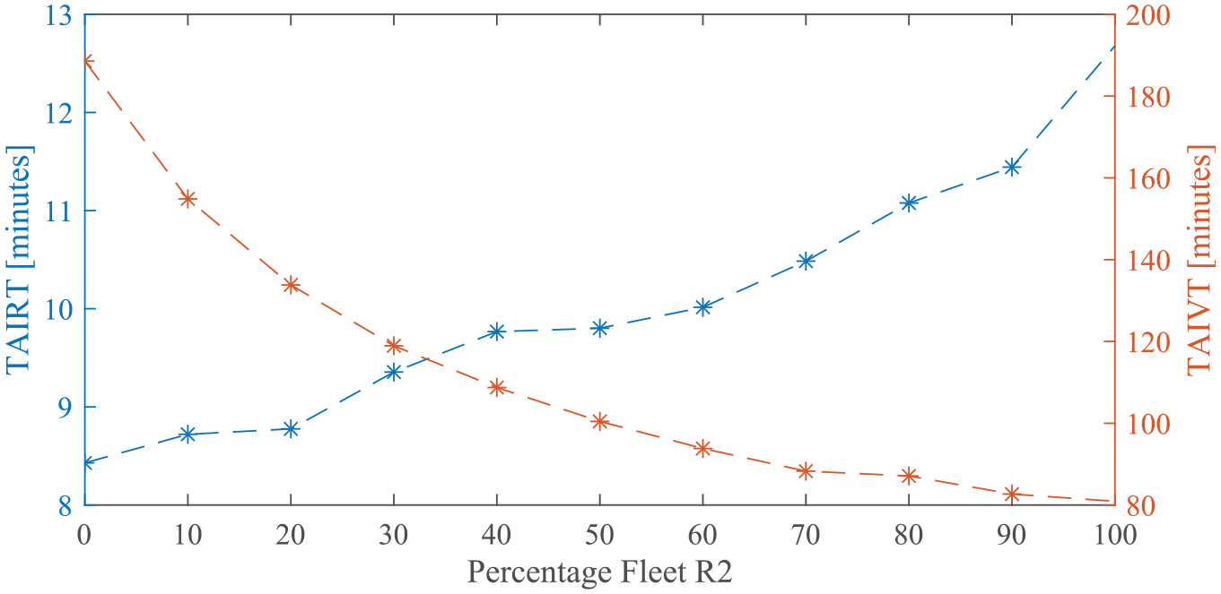
The TAIRT (blue) and TAIVT (red) achieved for a hybrid fleet (fleet size 224 vehicles). The bottom axis indicates the percentage of the fleet that patrol under R2, the remaining vehicles patrol under R1.

Future Simulation Improvements

The simulation has several simplifications, and future refinements should aim to further reflect the behavioral details of real-world TO patrols. For example, the simulated FTOs drove at a constant speed and we did not consider the effect of traffic congestion. Therefore, historical traffic data might be incorporated to reflect realistic driving conditions. In addition, the FTOs presently make an instantaneous routing decision at a node without changing their speed. Although this is reasonably realistic for TOs who choose to remain on the same highway, TOs who merge onto a different highway may slow down on a slip road or stop at a traffic-light controlled junction and thus incur a delay.

Future work should also improve the graphical highway network model on which the FTOs patrol in the simulation. Specifically, each edge distance should be modeled by the true driven distance between its start and end nodes (currently modeled by the node-to-node straight-line distance), and the model should capture junction size and drive-through structure.

Presently, we model the number of incidents on an edge as being proportional to its driven distance, with a constant of proportionality that is common to the entire network. However, an improved incident model might be calibrated with historical data concerning the number of incidents attended by TOs on each highway section. Although public road safety data sets exist that record the number of vehicle crashes and collisions across the SRN ( 56 ), TOs respond to several other types of incidents (breakdowns and removing abandoned vehicles, for example). Therefore, efforts should be made to liaise with highway agencies to determine the number of incidents attended by TOs at a section-by-section level. In addition, a more realistic incident model might also consider incidents with varying severity, thus with different TTCs that potentially require multiple TOs to attend. Such an incident model might require a more sophisticated incident response mechanism than the BWNN heuristic employed in this study.

There are several other possible operational constraints on the TO patrols that were not considered in our simulations, such as maximum mileage constraints. In addition, the FTOs in our simulations were all assumed to patrol under the same regime. In reality, TOs may have varying roles; for example, only some of the RWS Weginspecteurs may compile official incident reports. Therefore, future work might incorporate nonhomogeneous FTO fleets, using different patrol regimes.

R1 is designed for fast response to incidents that the RCC has been alerted to (e.g., via CCTV cameras), which then assigns the nearest TO. However, TOs patrolling under R2 may provide a faster response to minor incidents that are unknown to the RCC (e.g., in a CCTV blind spot or not reported by the public), which are not modeled in this paper. Such incidents are only discovered when TOs drive past them—an event promoted by maximizing the fleet’s coverage for TAM. Therefore, future simulations should consider mixtures of known and unknown incidents and whether combinations of different patrol regimes result in reduced IRTs overall.

Implementation of an Operational System

Our proposed concepts of operation assume that the SRN and FTO vehicles are equipped with the necessary communications infrastructure for the FTOs to patrol under each regime. When an FTO makes a routing decision (under either R1 or R2) they require real-time data; R2 requires the edge intervisit times, and R1 requires knowledge of the nearby FTOs and nodes around each FTO. Through dialogue with HE, it is understood that each RCC already captures live telemetry data for HE TO vehicles via an installed GPS-enabled device (HE, personal communication). Therefore, the data required by either regime can be computed in real-time (the intervisit times would be updated as a TO drives along a highway section) with the current technology.

To implement an operational system, a highway agency must decide how to compute and communicate the navigation instructions to each TO. This may be achieved in one of two ways:

The routing decision for each TO is computed in the RCC and then communicated back to the TO, either by radio or a connected (vehicle to RCC) navigation system; or,

The required data are sent back to the TO vehicle and a routing decision is computed by a small device installed in the vehicle.

Although each HE TO vehicle is already equipped with a dash cam, and thus may readily capture digital imagery data, future work must consider where and how the collected data would be analyzed in a deployed capability. There are seemingly three available options; the data may be analyzed either

In the TO vehicle,

At the roadside, or

At a central facility.

Option 1 would require a small computing device within the TO vehicle; data would then be sent directly from the dash cam to the device for analysis. The analysis would be fully automated, so that the TOs may continue to patrol as usual. Alternatively, miniaturized computers (e.g., a Raspberry Pi [ 57 ]) could be equipped with a camera, and thus might replace the dash cam completely. Then, for example, the computer vision-based TAM system developed by Strain et al. could be run in real-time during the TO patrol ( 5 ).

Option 2 would require installation of additional highway infrastructure, whereby a TO vehicle may wirelessly upload the collected asset data (via a connected device in the vehicle) to a computer installed on the roadside (i.e., edge computing technology [ 58 ]), where it is then automatically analyzed. Option 3 would instead transmit the data from the roadside to a central computer in an agency facility, accessible to an agency analyst and thus the data maybe analyzed manually or automatically. The results of the automatic analysis performed by Option 2 may be provided to an analyst via transmission from the roadside infrastructure to a central computer, whereas the results from Option 1 must first be uploaded to the roadside infrastructure.

Conclusion

In this paper, patrol routing strategies were proposed and simulated to consider whether a fleet of TOs could be used for TAM alongside their primary role of incident management. A case study of the HE TO fleet on the SRN in England, UK, was considered to investigate, as a proof-of-concept, whether data from dash cams installed in TO vehicles might be used to frequently capture asset data across an entire highway network.

Junction-to-junction links in the HATRIS data set were used to build a graphical model of the SRN. A simulator was built to deploy the HE TO fleet who responded to dynamically generated incidents. In the absence of data (e.g., incident TTC distribution and granular traffic speed data) across the entire SRN, the simulation made several assumptions and simplifications, including constant TO speed, an incident response mechanism that assigns the single nearest TO to each incident, and a constant incident TTC; thus the simulation presents several potential avenues for future refinements. Nonetheless, our simulation provided an initial (simplified) model with which we were able to investigate the principle focus of this paper: can TOs capture asset data alongside incident response?

Within the simulation, TOs patrolled under one of three regimes that influenced their routing decisions at each node (junction). The regimes considered were response, coverage, and random. The first aimed to minimize the fleet’s incident response time and act as a best case to compare with the other regimes’ IRTs. The second aimed to maximize the fleet’s coverage for asset management. The third regime, in which TOs make random routing decisions, acted as a base case.

To determine the feasibility of the proposed patrol routes, the IRTs and the edge intervisit times were computed. Overall, our simulations showed that the TOs (with varying fleet sizes) were able to monitor assets across the SRN while only increasing the incident response time by a few minutes.

We have demonstrated that TOs could be used for frequent asset data capture, alongside their primary role of incident response. To employ our proposed patrol routing strategies in operation, the increase in incident response time must be weighed up by decision makers. That said, in 2019, only 18% of accidents on major SRN highways (i.e., those highways with an “M” prefix) were categorized as “fatal” or “serious” ( 56 ), and thus, the majority of incidents that TOs attend (which also include breakdowns and other minor issues) are not time-critical. Highway agencies also need to consider the cost of the required sensor and communications infrastructure. However, note that for the HE TO fleet considered in this paper, the required sensing capability (the dash cams) and much of the communication infrastructure (e.g., radio and telemetry data sent to a regional control center) is already in place.

Footnotes

Acknowledgements

The authors acknowledge the support provided by Jacobs, Highways England, and the Engineering and Physical Sciences Research Council that have made the work presented in this paper possible.

Author Contributions

The authors confirm contributions to the paper as follows: study conception and design: T. Strain, R. E. Wilson, R. Littleworth; data collection T. Strain, R. E. Wilson, R. Littleworth; analysis and interpretation of results: T. Strain, R. E. Wilson, R. Littleworth; draft manuscript preparation: T. Strain, R. E. Wilson, R. Littleworth. All authors reviewed the results and approved the final version of the manuscript.

Declaration of Conflicting Interests

The authors declared no potential conflicts of interest with respect to the research, authorship, and/or publication of this article.

Funding

The authors disclosed receipt of the following financial support for the research, authorship, and/or publication of this article: This work was supported by a National Productivity Investment Fund (Award number 2107418) with contributions from Jacobs.

ORCID iDs

Tom Strain

Roger Littleworth

References

Highways England. Customer Service and Operations. Careers, 2020. https://careers.highwaysengland.co.uk/jobs-you-can-do/customer-service-and-operations. Accessed October 29, 2020.

U.S. Department of Transportation. Asset Management. Federal Highway Administration, 2021. https://www.fhwa.dot.gov/asset. Accessed March 1, 2021.

World Highways. IBI’s Routemapper Charts New Territory With Highways England. 2016. https://www.worldhighways.com/wh12/feature/ibis-routemapper-charts-new-territory-highways-england. Accessed May 10, 2021.

Browne

Life After SCANNER in Bristol. Highways Magazine, 2020. www.highwaysmagazine.co.uk/Life-after-SCANNER-in-Bristol/5465. Accessed May 10, 2021.

Strain

Wilson

R. E.

Littleworth

Computer Vision for Rapid Updating of the Highway Asset Inventory. Transportation Research Record: Journal of the Transportation Research Board, 2020. 2674: 245–255.

Golparvar-Fard

Balali

de la Garza

J. M.

Segmentation and Recognition of Highway Assets Using Image-Based 3D Point Clouds and Semantic Texton Forests. Journal of Computing in Civil Engineering, Vol. 29, 2015, p. 04014023.

Incident Management. The Highways Authority. 2021. https://www.incidentmanagement.nl/over+im/organisatie/default.aspx. Accessed June 9, 2021.

Pollitt

Highways Agency Puts Traffic Officers in the Driving Seat: Two Training Programs Help Patrols to Cut Motorway Congestion. Human Resource Management International Digest, Vol. 17, 2009, pp. 20–22. https://doi.org/10.1108/09670730910974314.

Highways England. Traffic Officer Manual. 2020. https://www.whatdotheyknow.com/request/341964/response/841566/attach/5/TO%20Manual%20Work%20Instructions%2008.07.16docx.pdf?cookie_passthrough=1. Accessed March 22, 2021.

10.

Highways England. Out With the Traffic Officers of Highways England – And What They do for Us. Linkedin, 2020. https://www.linkedin.com/pulse/out-traffic-officers-highways-england-what-do-us-simon-montague. Accessed March 22, 2021.

11.

Auto Express. What do Highways England Traffic Officers do all Day?2019. https://www.autoexpress.co.uk/107988/what-do-highways-england-trafficofficers-do-all-day-pictures. Accessed March 22, 2021.

12.

Bogatov

The Motorway Life in the Fast Lane, 3 The Need for Speed. 2016. https://www.youtube.com/watch?

13.

Highways England. Highways England Strategic Road Network Initial Report. 2017. https://assets.publishing.service.gov.uk/government/uploads/system/uploads/attachment_data/file/666857/Strategic_Road_Network_Initial_Report_Overview.pdf. Accessed March 3, 2021.

14.

Ebo Van Weel. Autodrip Nominated for Intertraffic Innovation Award 2016. 2016. https://www.ebovanweel.com/en/autodrip-nominated-for-intertraffic-innovation-award-2016. Accessed June 30, 2021.

15.

Polizei Brandenburg. Autobahnpolizei. 2021. https://polizei.brandenburg.de/liste/autobahnpolizei/62080. Accessed June 9, 2021.

16.

American Association of State Troopers. Highway Patrol/State Police Websites. 2020. https://www.statetroopers.org/useful-links/highway-patrol-state-police-websites. Accessed March 1, 2021.

17.

An Garda Síochána. Roads Policing. 2020. https://www.garda.ie/en/roads-policing/. Accessed March 22, 2021.

18.

Polizia di Stato. Le attivit`a della Stradale. 2021. https://www.poliziadistato.it/articolo/le-attivita-della-stradale. Accessed June 9, 2021.

19.

Steenbruggen

Kusters

Broekhuizen

Best Practice in European Traffic Incident Management. Procedia-Social and Behavioral Sciences, Vol. 48, 2012, pp. 297–310.

20.

Legislation.gov.uk. Traffic Management Act2004, c.18. 2004. https://www.legislation.gov.uk/ukpga/2004/18/contents?pt1-pb2-l1g4. Accessed March 22, 2021.

21.

New Civil Engineer. Motorway Traffic Officers Equipped to Deal With Cardiac Arrest. 2020. https://www.newcivilengineer.com/latest/motorway-traffic-officers-equipped-to-deal-with-cardiac-arrest-16-03-2020/. Accessed March 1, 2021.

22.

Dantzig

G. B.

Ramser

J. H.

The Truck Dispatching Problem. Management Science, Vol. 6, 1959, pp. 80–91.

23.

El-Sherbeny

N. A.

Vehicle Routing With Time Windows: An Overview of Exact, Heuristic and Metaheuristic Methods. Journal of King Saud University - Science, Vol. 22, 2010, pp. 123–131. https://doi.org/10.1016/j.jksus.2010.03.002.

24.

Pillac

Gendreau

Guéret

Medaglia

A. L.

A Review of Dynamic Vehicle Routing Problems. European Journal of Operational Research, Vol. 225, No. 1, 2013, pp. 1–11. https://doi.org/10.1016/j.ejor.2012.08.015. https://www.sciencedirect.com/science/article/pii/S0377221712006388.

25.

Wong

K. I.

Bell

M. G. H.

The Optimal Dispatching of Taxis Under Congestion: A Rolling Horizon Approach. Journal of Advanced Transportation, Vol. 40, 2006, pp. 203–220.

26.

Weintraub

Aboud

Fernandez

Laporte

Ramirez

An Emergency Vehicle Dispatching System for an Electric Utility in Chile. Journal of the Operational Research Society, Vol. 50, 1999, pp. 690–696. https://doi.org/10.1057/palgrave.jors.2600746.

27.

Lees-Miller

J. D.

Wilson

R. E.

Sampling of Redistribution of Empty Vehicles for Personal Rapid Transit. Transportation Research Record: Journal of the Transportation Research Board, 2011. 2216: 174–181.

28.

Reis

Melo

Coelho

A. L.

Furtado

Towards Optimal Police Patrol Routes With Genetic Algorithms. Proc., 4th International Conference on Intelligence and Security Informatics (ISI), San Diego, CA, 2006, pp. 485–491.

29.

Melo

Belchior

Furtado

Analyzing Police Patrol Routes With the Simulation of the Physical Reorganization of Agents. Proc., International Workshop on Multi-Agent Systems and Agent-Based Simulation, Utrecht, The Netherlands, 2005, pp. 99–114.

30.

Eriksson

Girod

Hull

Newton

Madden

Balakrishnan

The Pothole Patrol: Using a Mobile Sensor Network for Road Surface Monitoring. Proc., 6th International Conference on Mobile Systems, Applications, and Services, Breckenridge, CO, 2008, pp. 29–39.

31.

Carnelli

P. E.

Sooriyabandara

Wilson

R. E.

Large-Scale VANET Simulations and Performance Analysis Using Real Taxi Trace and City Map Data. Proc., 2018 IEEE Vehicular Networking Conference (VNC), Taipei, Taiwan, IEEE, New York, 2018, pp. 1–8. https://doi.org/10.1109/VNC.2018.8628352.

32.

Aslam

Lim

Pan

Rus

City-Scale Traffic Estimation From a Roving Sensor Network. Proc., 10th ACM Conference on Embedded Network Sensor Systems, Toronto, Ontario, Canada, 2012, pp. 141–154.

33.

Machado

Ramalho

Zucker

J.-D.

Drogoul

Multi-Agent Patrolling: An Empirical Analysis of Alternative Architectures. In Multi-Agent-Based Simulation II ( Simão Sichman

Bousquet

Davidsson

eds.), Springer, Berlin, Heidelberg, 2003, pp. 155–170.

34.

Agmon

Urieli

Stone

Multiagent Patrol Generalized to Complex Environmental Conditions. Proc., AAAI Conference on Artificial Intelligence, Vol. 25, San Francisco, CA, 2011.

35.

Iocchi

Marchetti

Nardi

Multi-Robot Patrolling With Coordinated Behaviours in Realistic Environments. Proc., 2011 IEEE/RSJ International Conference on Intelligent Robots and Systems (IROS), San Francisco, CA, IEEE, New York, 2011, pp. 2796–2801. https://doi.org/10.1109/IROS.2011.6094844.

36.

Government Buildings. UK Government Property and Land Database. 2021. https://governmentbuildings.co.uk. Accessed July 10, 2021.

37.

Highways England. Traffic Officer Fleet Vehicles. GOV.UK, 2020. https://assets.publishing.service.gov.uk/government/uploads/system/uploads/attachment_data/file/741217/FOI-765216_-_HE__Fleet__Vehicles_-_TO_Vehicles.csv/preview. Accessed October 30, 2020.

38.

Highways England. Where We’re Based. Careers, 2020. https://careers.highwaysengland.co.uk/how-we-work/where-we-re-based. Accessed November 6, 2020.

39.

Director General of the Ordnance Survey UK. A Brief Description of the National Grid and Reference System. His Majesty’s Stationery Office (HMSO), Richmond, UK, 1946.

40.

Highways England. Highways Agency Network Journey Time and Traffic Flow Data. GOV.UK, 2018. https://data.gov.uk/dataset/dc18f7d5-2669-490f-b2b5-77f27ec133ad/highways-agency-network-journey-time-and-traffic-flow-data. Accessed October 30, 2020.

41.

Highways England. Highways England Network Journey Time and Traffic Flow Data. GOV.UK, 2016. https://data.gov.uk/dataset/9562c512-4a0b-45ee-b6ad-afc0f99b841f/highways-england-network-journey-time-and-traffic-flow-data. Accessed October 30, 2020.

42.

Derrible

Kennedy

Applications of Graph Theory and Network Science to Transit Network Design. Transport Reviews, Vol. 31, No. 4, 2011, pp. 495–519. https://doi.org/10.1080/01441647.2010.543709.

43.

OpenStreetMap. Welcome to OpenStreetMap!2021. https://www.openstreetmap.org. Accessed June 10, 2021.

44.

Highways England. Our Roads. 2020. https://highwaysengland.co.uk/about-us/our-roads. Accessed October 30, 2020.

45.

Hall

R. W.

Incident Dispatching, Clearance and Delay. Transportation Research Part A: Policy and Practice, Vol. 36, No. 1, 2002, pp. 1–16.

46.

Rijkwaterstaat, Road Traffic Controller, 2022. https://werkenbij.rijkswaterstaat.nl/vakgebieden/weginspecteur/wegverkeersleider. Accessed June 21, 2022.

47.

Jovanis

P. P.

Chang

H.-L.

Modeling the Relationship of Accidents to Miles Traveled. Transportation Research Record: Journal of the Transportation Research Board, 1986. 1068: 42–51.

48.

Lord

Washington

S. P.

Ivan

J. N.

Poisson, Poisson-Gamma and Zero-Inflated Regression Models of Motor Vehicle Crashes: Balancing Statistical Fit and Theory. Accident Analysis and Prevention, Vol. 37, 2005, pp. 35–46. https://doi.org/10.1016/j.aap.2004.02.004.

49.

Caliendo

Guida

Parisi

A Crash-Prediction Model for Multilane Roads. Accident Analysis and Prevention, Vol. 39, 2007, pp. 657–670. https://doi.org/10.1016/j.aap.2006.10.012.

50.

Wang

Quddus

M. A.

Ison

S. G.

Impact of Traffic Congestion on Road Accidents: A Spatial Analysis of the M25 Motorway in England. Accident Analysis and Prevention, Vol. 41, 2009, pp. 798–808.

51.

Office of Road and Rail. Annual Assessment of Highways England’s Performance. ORR, 2019. https://assets.publishing.service.gov.uk/government/uploads/system/uploads/attachment_data/file/818764/annual-assessment-of-highways-englands-performance-2019-print.pdf. Accessed March 4, 2021.

52.

Ghosh

Savolainen

P. T.

Gates

T. J.

Examination of Factors Affecting Freeway Incident Clearance Times: A Comparison of the Generalized F Model and Several Alternative Nested Models. Journal of Advanced Transportation, Vol. 48, No. 6, 2014, pp. 471–485.

53.

Giuliano

Incident Characteristics, Frequency, and Duration on a High Volume Urban Freeway. Transportation Research Part A: General, Vol. 23, No. 5, 1989, pp. 387–396.

54.

Autocar. Highways Traffic-Officers - Meet the People Behind the Nicknames. 2020. https://www.autocar.co.uk/car-news/new-cars/highways-trafficofficers-meet-people-behind-nicknames. Accessed January 26, 2021.

55.

Highways England. Smart Motorways Stocktake: First Year Progress Report 2021. 2021. https://highwaysengland.co.uk/media/bb4lpkcp/smart-motorways-stocktake-first-year-progress-report-2021.pdf. Accessed June 10, 2021.

56.

Department for Transport. Road Safety Data. GOV.UK, 2020. https://data.gov.uk/dataset/cb7ae6f0-4be6-4935-9277-47e5ce24a11f/road-safety-data. Accessed March 28, 2021.

57.

Raspberry Pi Foundation. Teach, Learn, and Make With Raspberry Pi. 2022. https://www.raspberrypi.org/. Accessed January 21, 2022.

58.

Liang

Hatcher

W. G.

Lin

Yang

A Survey on the Edge Computing for the Internet of Things. IEEE Access, Vol. 6, 2018, pp. 6900–6919. https://doi.org/10.1109/ACCESS.2017.2778504.

Patrol Regimes for Traffic Officers in Transportation Asset Monitoring

Abstract

Keywords

Background and Literature Review

Traffic Officer Fleets

Vehicle Routing Problems

Mobile Sensing for a Secondary Purpose and Maximal Coverage Systems

Data Sources and Preparation

Traffic Officers

Outstations

Strategic Road Network

Graphical Highway Network Model

Concepts of Operation

Traffic Officer Patrol Regimes

Incident Response Mechanism

Simulation Methodology

Initialization and Time Stepping

Incident Model

Determination of Response Regime Parameters and Node Weightings

Simulation Metrics and Analysis

Simulation Run-In and Return Period

Simulation Results

Varying Fleet Sizes

Discussion

Future Simulation Improvements

Implementation of an Operational System

Conclusion

Footnotes

Acknowledgements

Author Contributions

Declaration of Conflicting Interests

Funding

ORCID iDs

References