Calibration of a Mechanistic-Empirical Cracking Model Using Network-Level Field Data

Abstract

At the core of a mechanistic-empirical (M-E) pavement design method is a collection of performance models that each predicts the development of a specific pavement distress, such as fatigue cracking and surface rutting. Each model has both mechanistic and empirical parts. The empirical parts need to be calibrated to remove bias and increase prediction accuracy. This process has traditionally been conducted with small numbers of field sections for which materials may or may not have been sampled and tested. This paper presents a new calibration approach that uses network-level field data and statewide distributions of material properties, without having to sample and test every individual calibration section. The calibration of the fatigue and reflection cracking models for CalME, the M-E design software developed for the California Department of Transportation, is used as an example to illustrate the new approach. The new approach works by correlating the statistical distributions of M-E design inputs with the statistical distribution of pavement performance, both at the network level. The uncertainties affecting pavement performance are divided into those specific to a given project (within-project variability) and those that vary between projects (between-project variability). This distinction allows a clear definition of design reliability. The results showed that the new approach can overcome some of the network-level data limitations and provides a reasonable calibration ready for routine pavement design.

At the core of a mechanistic-empirical (M-E) pavement design method is a collection of models that each predicts the development of a specific pavement distress. For example, the Pavement ME Design (PMED) program includes the following models for new flexible pavements: asphalt concrete (AC) top-down fatigue cracking, AC bottom-up fatigue cracking, AC thermal cracking, AC permanent deformation, pavement permanent deformation, and roughness (International Roughness Index [IRI]) ( 1 ). These models are typically referred to as performance models ( 2 ), which provide the results needed to determine whether a given pavement design is adequate against the distresses of interest.

Each performance model has three key components: a response submodel that estimates the critical mechanical response such as stress and strain that drives the damage related to the distress under consideration; a damage submodel that estimates the accumulation of said damage; and a transfer function that correlates the damage to the distress. Whereas the response submodels are typically based on rigorous mathematics and mechanics, the damage submodels and transfer functions are simplifications of complicated pavement behaviors and usually resort to empirical parameters to account for knowledge deficiencies and model imperfections. The response submodel is the mechanistic part of an M-E performance model, whereas the damage submodel and the transfer function together is the empirical part.

The empirical part of the performance models requires calibration to eliminate any bias and minimize the residual errors between observed or measured results from the real world ( 3 ). The residual errors are also used for reliability calculations that account for uncertainty of the models and calibration. In most M-E methods, including the PMED, uncertainty in design inputs is not explicitly accounted for. Uncertainty of design inputs differs between design-bid-build and design-build project delivery methods.

For PMED, the calibration is a two-step process: a global calibration using national data followed by a local calibration. Both calibrations can result in changes to damage submodels and transfer functions (2–5). There are also other local calibration efforts that only involve optimizing empirical parameters in the transfer functions ( 6 , 7 ).

Traditionally, calibrations of M-E performance models have been conducted with small numbers of field sections from which materials may or may not have been sampled ( 3 , 5–7). Although these calibrations have been shown to work reasonably well ( 7 ) or very well ( 5 ), some questions remain open:

• Is it necessary to sample and test the material for each of the sections included in the calibration dataset?

• How to account for the constant changes in materials and construction practices? As pointed out in one study ( 7 ), “new materials and new construction and rehabilitation technologies are emerging every year, if not every day. All of these will drive local calibration as a dynamic process.”

• How to account for the different levels of input between calibration and design? As suggested in one study ( 5 ), the design should use Level 1 (i.e., with detailed laboratory characterization of materials) inputs as much as possible as the calibration was done using Level 1 inputs. Does this mean the calibration needs to be conducted separately for each of the input levels?

• How to properly account for design reliability?

These questions prompted the authors to seek and develop an alternative approach for the calibration of M-E design methods for the California Department of Transportation (Caltrans), which uses CalME ( 8 ) for flexible-surfaced pavements and PMED for rigid pavements. This approach has been successfully applied to both CalME and PMED; this paper covers CalME only.

Similar to PMED, CalME calibration is also a two-step process but each covers a different part: calibration of the damage submodel followed by calibration of the transfer function. The damage submodels have been calibrated using data from well-controlled, well-instrumented datasets from accelerated pavement test sections ( 9 , 10 ). This paper covers the calibration of transfer functions only, referred to hereafter as field calibration.

The network-level data used in this paper come from the Caltrans pavement management system (PMS). These data have undergone rigorous quality control but are by no means perfect. Although these data have limitations (lack of material test data, inaccuracy in traffic volume, and irregularities in observation interval), they offer orders of magnitude more performance data than small numbers of test sections and are the key to a “big data” type of calibration approach.

This paper provides a detailed explanation of the alternative M-E calibration approach and uses the cracking model in CalME as an example of how it works. The paper also suggests some areas for improvement of this approach. More details can be found in the report ( 11 ) that this paper summarizes.

Alternative Approach for Calibration of Transfer Function

The alternative calibration approach starts with the assumption that the M-E performance model under consideration accurately describes the pavement behavior under calibration. In addition, the inputs to the model for each pavement section are assumed to have random variations from different sources that can be modeled. With these assumptions, Monte Carlo simulations can be used to determine the expected distribution of pavement performance, from which a way to identify transfer function parameters was found.

Damage Submodel for Asphalt Concrete Fatigue Cracking

The CalME AC fatigue cracking model uses a multi-layer elastic program ( 12 ) as the response submodel. In CalME, only traffic-related fatigue damage is considered. Details of the model can be found in the report ( 11 ). The key part of the model is the following equation for estimating fatigue life MNp:

$$M{N}_p=A\times {\left(\frac{\epsilon }{{\epsilon }_{\mathrm{ref}}}\right)}^{\beta }\times {\left(\frac{E}{E_{\mathrm{ref}}}\right)}^{\beta /2}$$

where

$\epsilon$ is the bending strain at the bottom of the asphalt layer, negative for tensile,

E is the mix stiffness,

$\epsilon$ _ref  = −200 microstrain (−200 $\times {10}^{-6}$  in./in.) is the reference bending strain,

E_ref = 3,000 MPa (435 kips per square inch [ksi]) is the reference stiffness, and

A and β are material dependent model parameters.

Transfer Function for Asphalt Concrete Fatigue Cracking

Once the fatigue damage is determined, the percent of wheel path cracked, denoted as CRK, is assumed to relate to the fatigue damage through the following transfer function:

$$\mathrm{CRK}=\frac{100}{1+{\left(\frac{\omega }{{\omega }_{50}}\right)}^{\beta }}$$

where $\omega$ is the calculated fatigue damage, and ${\omega }_{50}$ and $\beta$ are model parameters to be determined through field calibration. ${\omega }_{50}$ represents the fatigue damage corresponding to 50% wheel path cracking.

Each parameter may depend on additional factors such as pavement structure type, climate condition, hot mix asphalt (HMA) layer thickness. Note that ${\omega }_{50}$ depends on the physical meaning of the fatigue damage predicated by the model used and it can be any value between 0 and 1.0.

The assumed transfer function represents an s-shaped curve that seems to match observed cracking progression in the field. The mid-portion slope of the s-shaped curve is controlled by $\beta$ . Accordingly, $\beta$ is called the shape parameter, and it is always negative, with a higher absolute value suggesting steeper ascent.

Within-Project and Between-Project Variability

There are two contributors to variations in project performances: within-project variability (WPV) and between-projects variability (BPV). WPV occurs within a given project and comes from variation of the subgrade, and variability of construction using the given set of materials that a contractor brings to the project. BPV is the uncertainty in a design-bid-build project in relation to which contractor will win and the specific materials they will deliver. More discussion of WPV and BPV can be found in Wu et al. ( 11 ).

Project-Level Performance and Calibration

In this section, Monte Carlo simulations are run at the project level using WPV in a simple example to demonstrate the process. This example is greatly simplified from the way traffic and materials are characterized in CalME. The Monte Carlo simulations are done using a script written in Matlab that implements the fatigue cracking model.

Simple Project Example

The pavement in the project is assumed to have three layers with 120 mm (0.4 ft) of AC over 300 mm (1.0 ft) of aggregate base (AB) over subgrade. The AB and subgrade layers have constant stiffnesses of 300 MPa (43.5 ksi) and 50 MPa (7.25 ksi), respectively. The AC layer is viscoelastic, but the loading temperature and loading frequency are assumed to be constant at 20°C (68°F) and 10 Hz for this example (stiffness master curves are used in CalME). The statewide median AC mix with PG 64 binder from the CalME standard materials library is used for the AC layer.

Traffic is applied with standard equivalent single axles (i.e., 80 kN [18 kips] single axles with dual tires) for this example (axle load spectra are used in CalME).

The WPV for the project is assumed to come from only two sources in this example: the initial stiffness of the AC layer, denoted as E, and the fatigue model parameter A for the AC layer. Both E and A are assumed to follow lognormal distributions. Specifically, E has a mean value of 3,000 MPa (435 ksi) and a standard deviation of 600 MPa (87.0 ksi) (i.e., E∼LN[3000, 600], where LN[P₁,P₂] indicates a random variable following lognormal distribution with mean P₁ and standard deviation P₂). Parameter A has a mean value of 150 and a standard deviation of 60 (i.e., A∼LN[150,60]).

To conduct a Monte Carlo experiment, a project is divided into many segments (5,000 was found to be statistically stable) and each segment has a constant pair of values for (E, A) determined by random sampling from the respective distribution. The transfer function parameters used were ${\omega }_{50}=0.10$ and $\beta =-5.0$ , respectively.

Monte Carlo Simulation Results and Observations

Figure 1 shows the cracking histories for the different segments within the project and the overall average and median. Each of the individual curves is a transformed version of the transfer function because the fatigue damage is a monotonic function of the traffic applied in this case. The significant difference between different segments illustrates the effect of WPV (i.e., the variability of $(E,A)$ for this example project).

Figure 1.

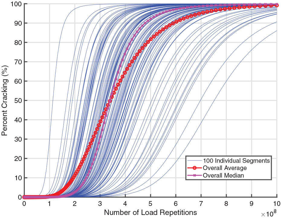
Cracking histories for individual segments (only showing 100 out of 5,000 segments used) and the project overall average and median.

The overall average shown in Figure 1 is the performance data typically collected in pavement condition surveys. Figure 1 indicates that the shape of the cracking history curve for individual segments is very different from the shape of the overall average curve: the overall average curve is much flatter than the curves for individual segments.

Figure 1 also shows the overall median performance, which was determined by finding the median of percent cracking among all segments at any given time. Unlike the overall average, the overall median has the same shape as the individual segments. This is because pavement performance is a monotonic function of different inputs. This general trend is hereafter referred to as the monotonic property of pavement systems.

It can be deduced that increasing the fatigue model parameter A always leads to longer pavement cracking life if all other inputs are equal. The effect of stiffness depends on the pavement structure, primarily AC thickness, and in this example increasing stiffness leads to lower cracking life (at some point as the AC thickness is increased, this reverses and greater stiffness results in longer life). The interaction of A and E for a given material is not yet considered in this example.

Figure 1 shows a striking feature: the overall average and overall median reach 50% simultaneously, which is not a coincidence. Specifically, the overall average is essentially the cumulative distribution function (CDF) of cracking life for the project. The number of load repetitions to 50% cracking on the overall average curve therefore is the median cracking life of the project, which only depends on the median of $(E,A)$ because of the monotonic property. Because the overall average converges to the overall median as the WPV decreases to zero, the overall median is technically a special case of the overall average and, therefore, must go through the same point at 50% cracking. This feature can be used to determine ${\omega }_{50}$ .

Effects of Different Within-Project Variability

The effect of WPV on the expected pavement performance is illustrated in Figure 2. Although all going through the same $N_{50}$ (number of load repetitions to 50% cracking), the overall average cracking curves change shape with the amount of WPV. The higher the WPV, the more spread out the pavement performance is, as indicated by the flatter slope of the middle portion of the overall average cracking curves. In other words, the slope of the mid-portion of each overall average cracking curves provides an upper bound estimate of the shaper parameter $\beta$ of transfer function.

Figure 2.

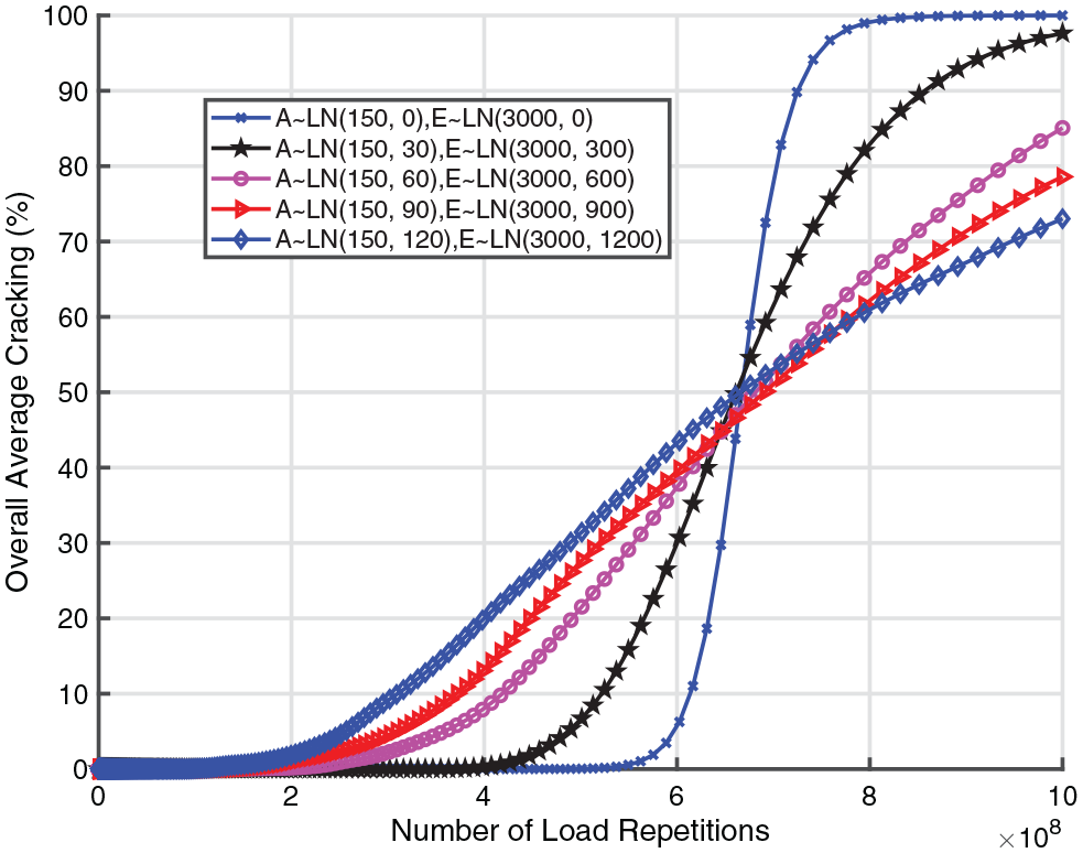
Overall average cracking histories for projects with different standard deviations for inputs.

Project-Level Observations and Calibration Procedure

In summary, the time to reach 50% cracking (i.e., $t_{50}$ ) for each segment only depends on the median values of M-E inputs, whereas the shape of the overall average cracking history curve reflects the amount of WPV, which is a function of the variability of the M-E inputs. If the statistical distributions of all the M-E inputs for a given project are known, the transfer function can be identified through the following steps:

• The damage corresponding to $t_{50}$ , denoted as ${\omega }_{50}$ in the transfer function, can be calculated using the project median M-E inputs.

• The shape parameter $\beta$ of the transfer function, can be back-calculated by running Monte Carlo simulations and finding the best match between the simulated overall average cracking curve and the observed one using WPV of the M-E inputs.

Statewide Network-Level Performance and Calibration

The Monte Carlo simulations are conducted at the statewide network level by building a network of simple projects similar to the one used above.

Simple Network Example

At the network level, the median values of $(E,A)$ for individual projects are expected to follow their own layer of random distributions, especially if the network is large enough to have multiple sources of materials. In this section, the expected network-level performance is again illustrated by running Monte Carlo simulations. The following simplifying assumptions are used to produce a simple network example for this paper:

• The median value of $E$ for projects in the network is randomly chosen between 3,000 MPa (435 ksi) and 7,000 MPa (1,015 ksi) at 500 MPa (72.5 ksi) intervals (i.e., nine values in total).

• The coefficient of the standard deviation of $E$ in each project is fixed at 0.2 for all projects.

• The median value of $A$ is randomly chosen between 75 and 300 for all projects in the network, uniformly distributed in log space with eight intervals in between (i.e., nine values in total).

• The coefficient of the standard deviation of $A$ in each project is fixed at 0.4 for all projects.

Note that the specific values selected here should not affect the generality of the findings derived from this example. The assumed CDFs for E and A are shown in Figures 3 and 4, respectively.

Figure 3.

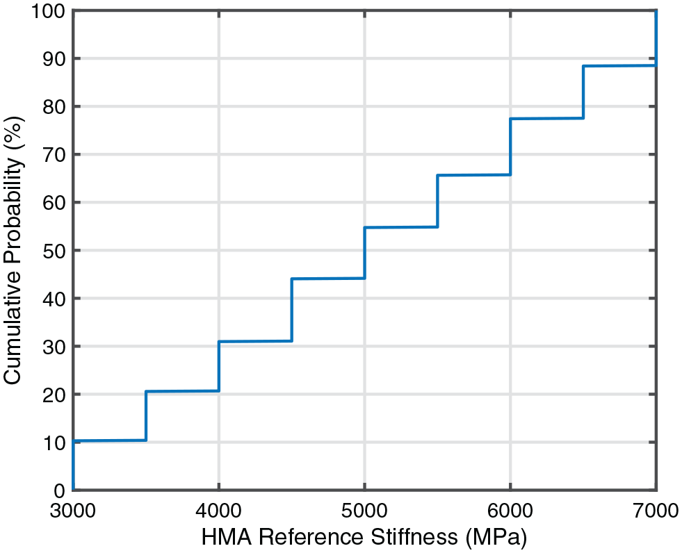
Cumulative distribution function of the median value of E for projects in the network.

Figure 4.

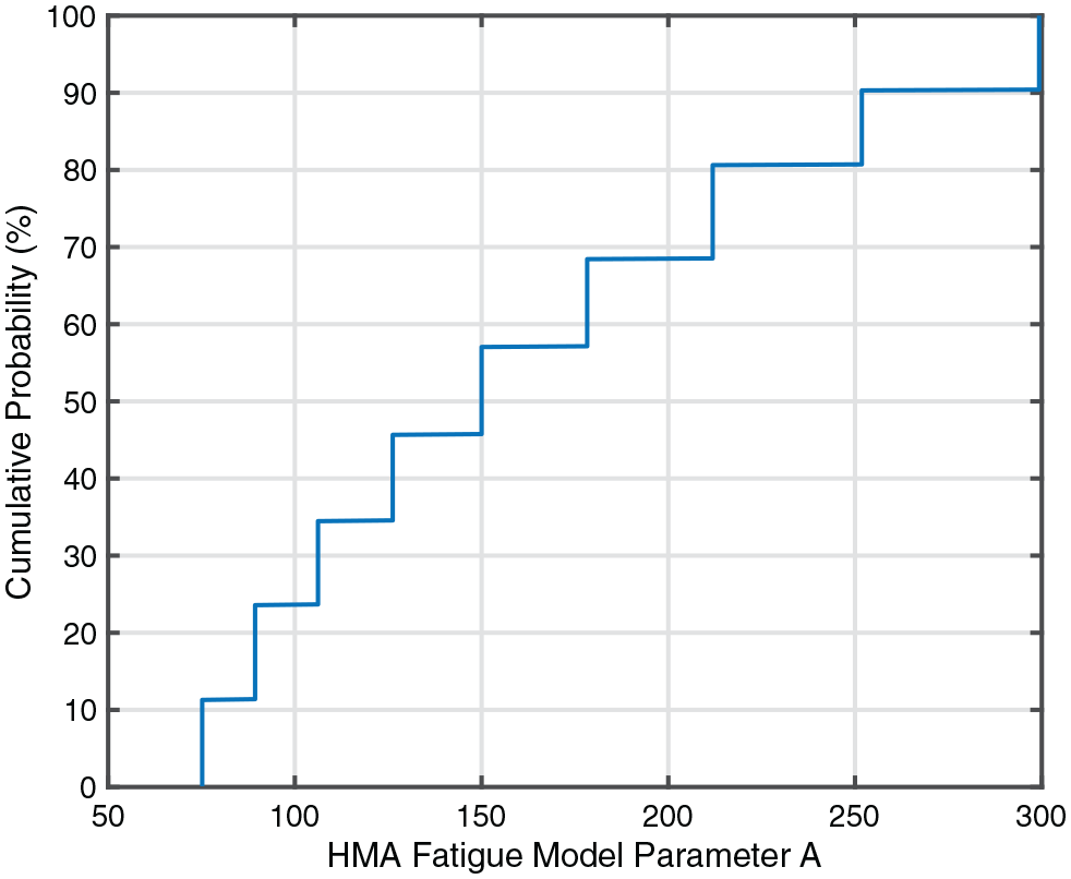
Cumulative distribution function of the median value of fatigue model parameter A for projects in the network.

Monte Carlo Simulation Results and Observations

Figure 5 shows the simulated overall average cracking histories for 1,000 individual projects in the example network and the one for a project with the network median inputs (NMI), which in this case are 5,000 MPa (725 ksi) for $E$ and 150 for $A$ .

Figure 5.

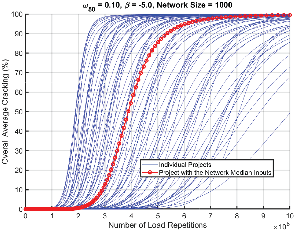
Overall average cracking histories for individual projects in the network and for the project with the median inputs.

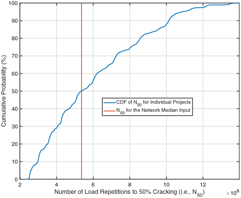
For every project in Figure 5, there is a corresponding $N_{50}$ that reflects the median value of $(E,A)$ for the given project. As expected, and illustrated in the figure, the performance of the project with NMI is somewhere in the middle among all projects in the network. The $N_{50}$ of the project with NMI is the same as the network median $N_{50}$ , with minor differences likely as a result of rounding errors in Monte Carlo simulations, as illustrated in Figure 6.

Figure 6.

Cracking performance of individual projects and the project with the network median input.

As mentioned above, ${\omega }_{50}$ was set to 0.10 in Monte Carlo simulations here. This value must be estimated without knowing the actual value of $(E,A)$ for each individual project for field calibration. The following are known, however:

• $N_{50}$ of each individual project (or an estimate based on extrapolation of cracking history)

• NMI of the given network

The hypothesis that the fatigue damage in the AC layer for the project with NMI is equal to the true ${\omega }_{50}$ after applying load repetitions equal to the median $N_{50}$ of the network was tested with multiple rounds of network-level Monte Carlo simulations. The relative error in estimated ${\omega }_{50}$ is shown in Figure 7, which shows that the error in estimated ${\omega }_{50}$ ranges from 1 to 6 percent and although not always, generally decreases with the increase in network size, especially after the network size exceeds 400 to 800. It is therefore concluded that this hypothesis is true and provides a reasonable way to estimate ${\omega }_{50}$ from network-level data.

Figure 7.

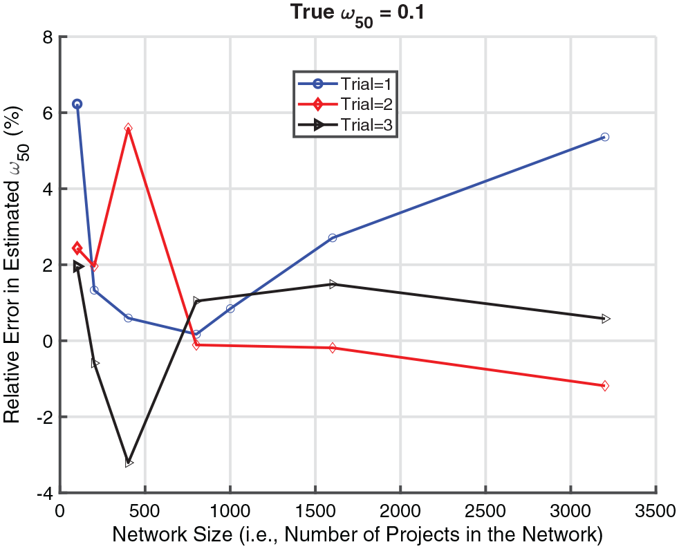
Effect of network size on the relative error in estimated ${\mathit{\omega }}_{50}$ .

The variability between different projects (i.e., the BPV) in relation to the M-E inputs in the network can be evaluated by reviewing the distribution of the following normalizing factor:

$$c_n=\frac{N_{50}}{{\tilde{N}}_{50}}$$

where ${\tilde{N}}_{50}$ is the network median of $N_{50}$ . Note that in actual calibration, the time to 50% cracking ( $t_{50}$ ) is more practical than $N_{50}$ , so the alternative definition should be used when considering a smaller set of data for which the traffic volume is roughly the same:

$$c_n=\frac{t_{50}}{{\tilde{t}}_{50}}$$

Figure 8 shows the CDF function of $c_n$ for this simulated network. For easier reference, $c_n$ is hereafter referred to as the relative performance factor (RPF). As expected, the 50^th percentile of $c_n$ is exactly 1.0. This chart provides a way to account for the BPV if one were to use NMI to design pavements. For example, the 5th percentile of $c_n$ is approximately 0.5 according to Figure 8, which means that one can achieve 95% reliability in relation to BPV by multiplying the $N_{50}$ predicted using NMI by 0.5 as the pavement design $N_{50}$ .

Figure 8.

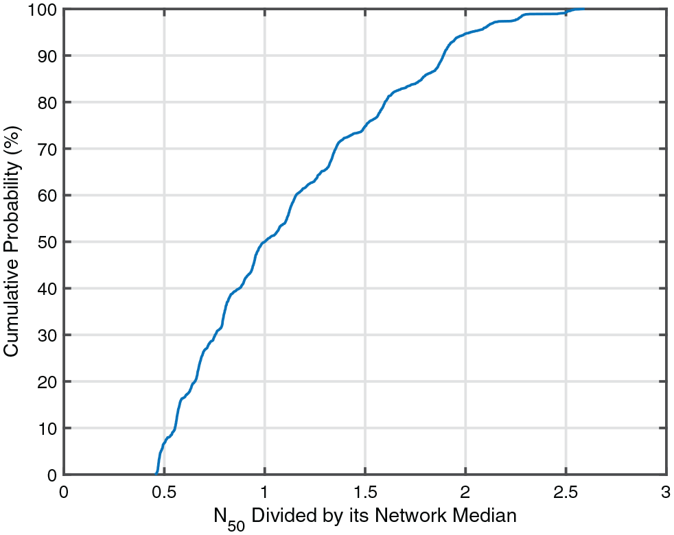
Cumulative distribution function of the normalizing factor.

Network-Level Calibration Procedure

Based on the observations from the example network-level Monte Carlo simulations, the transfer function can be identified with the following steps using the network-level data:

1. Review M-E inputs for the statewide network and determine the NMI, and the typical standard deviations.

2. Determine $t_{50}$ , and $\beta$ as the slope of the observed cracking history curve at $t_{50}$ for each project within the network.

3. Determine the observed network median $t_{50}$ using the results from Step 2.

4. Simulate the pavement with NMI but without any WPV to determine the damage in the HMA layer corresponding to the network median $t_{50}$ determined in Step 3 to obtain the estimated (i.e., calibrated) ${\omega }_{50}$ for the transfer function.

5. Review the slopes determined in Step 2 and select the proper percentile of the slope for use in design ( ${\beta }_{\mathrm{design}}$ ) considering the desired reliability level. A steeper slope corresponds to low WPV, which means better construction quality control. The lowest slope provides a preliminary estimate of the shape parameter $\beta$ of the transfer function.

6. The design WPV can be back-calculated by running Monte Carlo simulations sampling from the distributions of a selected set of critical inputs and matching the slope of ${\beta }_{\mathrm{design}}$ selected in Step 5.

7. Calculate the normalizing factor $c_n$ for each project, then find the percentiles corresponding to different desired reliability levels for design. These percentiles can be used as multipliers on design life estimated using NMI to account for different design reliabilities accounting for BPV.

The highway network may need to be sub-divided into calibration cells based on structure type (new pavements, AC overlay over old cracked flexible pavements, etc.), AC layer thickness, traffic level, climate zone, and so forth. The procedure outline above can then be applied to each of the calibration cells. The calibration results can then be grouped and simplified for use in the actual design.

Performance Data

Network-level performance data were extracted from the Caltrans PMS for the field calibration. The dataset was divided into short lane-by-lane segments with uniform construction histories, traffic, and climate. With its associated performance time history, each of these uniform segments served as a basic unit for field calibration and are hereafter referred to as “virtual projects.” The data being used for calibration of asphalt pavements are summarized in Table 1, and are grouped by structure types. Each structure type is called a sub-network.

Table 1.

Pavement Management System Performance Data for Calibration

Abbreviation	Pavement type	Number of virtual projects	Lane-km (lane-mile)	Observation period
N-AB	New asphalt pavement with aggregate base	8,350	1,711 (1,063)	1978–2014
N-CB	New asphalt pavement with cemented bases	1,366	259 (161)	1978–2014
R-FP	Asphalt overlays on old flexible pavements	253,841	55,846 (34,703)	1978–2014
R-RP	Asphalt overlays on old concrete pavements	7,877	2,255 (1,401)	1978–2014
R-PDR-EA	Rehabilitation of flexible pavements using partial-depth reclamation with engineering emulsion	6,717	1,435 (892)	1978–2018
R-FDR-FA	Rehabilitation of flexible pavements using full-depth reclamation with foam asphalt	1,431	280 (174)	1978–2018
R-FDR-C	Rehabilitation of flexible pavements using full-depth reclamation with cement	19	10 (6)	1978–2020

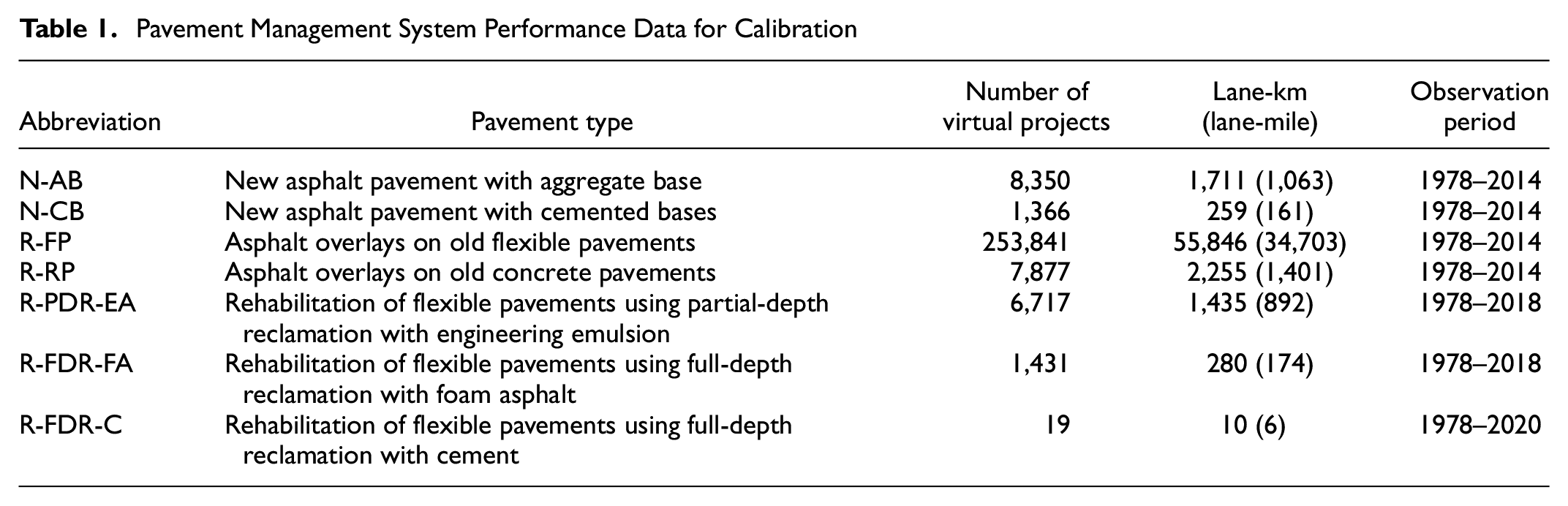
Note that for some sub-networks, reflective cracking is more dominant than fatigue cracking. The CalME model for reflective cracking are explained in Wu et al. ( 13 ). Surface cracking is the combination of fatigue and reflective cracking. It can be seen the number of projects and the segment lengths are orders of magnitude larger than those possible using traditional calibration approaches.

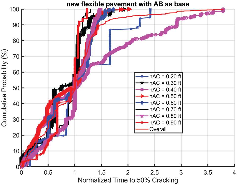
Determination of Time to 50% Cracking

Pavements usually have undergone some maintenance or rehabilitation before reaching 50% cracking. It is therefore necessary to introduce a procedure to provide a reasonable estimate of the time to 50% cracking (i.e., $t_{50}$ ). After some trial and error, it was found that $t_{50}$ of virtual projects can be determined reasonably well by fitting and extrapolating the observations for each virtual project using the following rules:

• The correlation between time in years and percent wheel path cracked has the same functional form as the transfer function.

• The observed time history needs to be constrained with two data points: 0% cracking at year zero and 99% cracking at year 50.

The constraint at year 50 is arbitrary but is believed to be reasonable as a flexible pavement is not expected to last more than 50 years in the performance dataset used where projects have 10- or 20-year design lives. Figures 9 and 10 show two examples of the extrapolation: one with extensive observed cracking and the other showing no cracking during any observations of its performance data.

Figure 9.

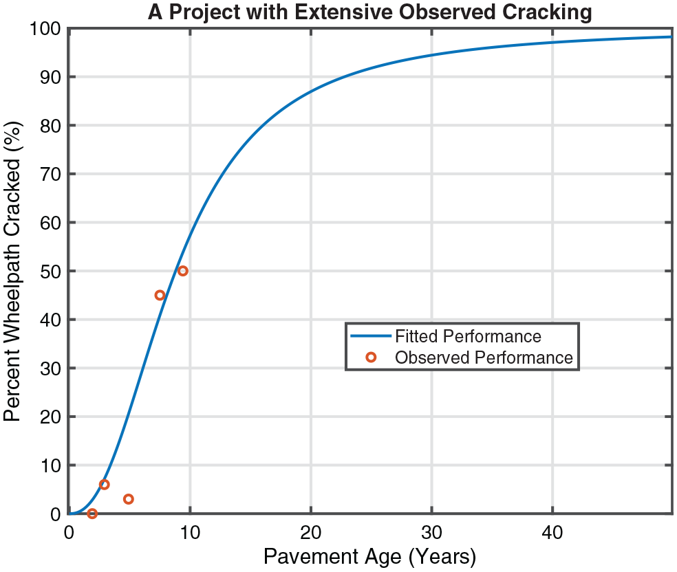
A project with extensive observed cracking and an extrapolated $t_{50}$ of 8.8 years.

Figure 10.

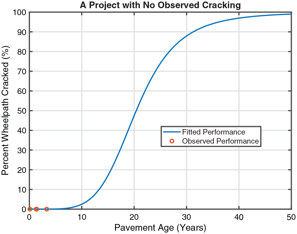
A project with zero observed cracking and an extrapolated $t_{50}$ of 20.4 years.

Limitations of the Data

Not all variables that are important to pavement performance are recorded in the Caltrans PMS database. The following are some of the limitations:

• For new flexible pavements: there are no data for the subgrade type.

• For rehabilitation projects: there are no data for the existing underlying structure other than the milling depth.

• There are no records for the performance-related mechanical properties of the AC and other layers (such as fatigue resistance of the AC layer, stiffness of the AB layer) of the materials used.

These were handled by using NMI to represent typical scenarios, with the uncertainties accounted for as part of the BPV.

In addition, the data are not uniformly distributed across critical variables such as total AC thickness, climate, and traffic volume.

Calibration and Results

Not all details of the calibrations can be included in this paper because of length limitations. A discussion of the NMI is first presented, followed by the calibration steps and results for the N-AB sub-network defined in Table 1, as an example for the other structure types. As mentioned earlier, more details can be found in the report ( 11 ).

Network Median Input

As explained earlier, the new calibration approach needs to estimate the NMI for the critical variables that are not recorded, such as the layer materials and bonding conditions.

Surface Layer Material and Bonding Condition

The AC surface materials on the Caltrans highway network have changed over the last 30 years with changes in mix design procedures and use of rubberized binder, among other things. The following is a summary of Caltrans HMA practices that were incorporated into the simulations for projects constructed in different time periods:

• Before 2000: Before implementation of HMA QC/QA specifications. Data show that average air-void contents were about 11%, and that a high percentage of multi-lift paving had poor bonding from lack of multi-lift paving tack coat requirements ( 14 ).

• 2000 to 2015: After QC/QA specification implementation and better tack coat requirements. Data showed that the average air-void contents were about 7% ( 14 ) and better bonding was seen. There was rubberized mix usage on most surfaces, with a 0.20 ft (60 mm) maximum thickness, and HMA underneath.

• 2015 to present: Change to Superpave mix design method, with generally increased binder contents and better fatigue performance ( 15 ).

It was decided to use a weighted average performance of these historical mixes from the Caltrans/UCPRC database to represent the asphalt layer behavior, in relation to the NMI for AC properties for each time period.

Non-Surface Layer Materials

No mechanical properties for aggregate bases, cement-treated bases and subgrade are recorded in the PMS database. The typical material properties for these non-surface layers in the historical Caltrans network were determined based on a combination of historical deflection and laboratory testing data and engineering judgment.

N-AB: New Flexible Pavements with Aggregate Base

Sensitivity of CalME Fatigue Cracking Model

A sensitivity study (see Wu et al. [ 11 ]) suggests that overall, the critical variables for this structure type include surface type, traffic volume, asphalt-bound-layer bonding condition, and AC thickness. Relatively speaking, the cracking performance is not sensitive enough to base thickness, subgrade type, or climate zone to consider in the calibration of the transfer function, although these variables do need to be considered in project design.

Calibration Cells

Based on the sensitivity study, the PMS data was divided into calibration cells based on AC thickness and truck traffic volume. Then, the NMI and the value of ${\omega }_{50}$ were determined for each combination of AC thickness and truck traffic volume that had PMS data.

Determination of Network-Level Critical Damage ${\mathrm{\omega }}_{50}$

Once the ${\omega }_{50}$ was calculated for each calibration cell, the plan was to then review the correlation between ${\omega }_{50}$ and traffic volume as well as surface layer thickness to identify any trends. However, this approach was found to lead to unreasonably high sensitivity between ${\omega }_{50}$ and traffic volume. Considering known uncertainties in relation to past traffic data, endemic to all M-E calibration methods, more importance was placed on AC thickness.

The initial step was to pool the PMS data for the same surface layer thickness regardless of the recorded traffic volume. This allowed identification of a trend line for the correlation between calibrated ${\omega }_{50}$ and AC thickness by adjusting the traffic volume for each AC thickness. The distribution of the resulting traffic volume estimates was then reviewed for consistency with the recorded values. This process is further illustrated in Figure 11.

Figure 11.

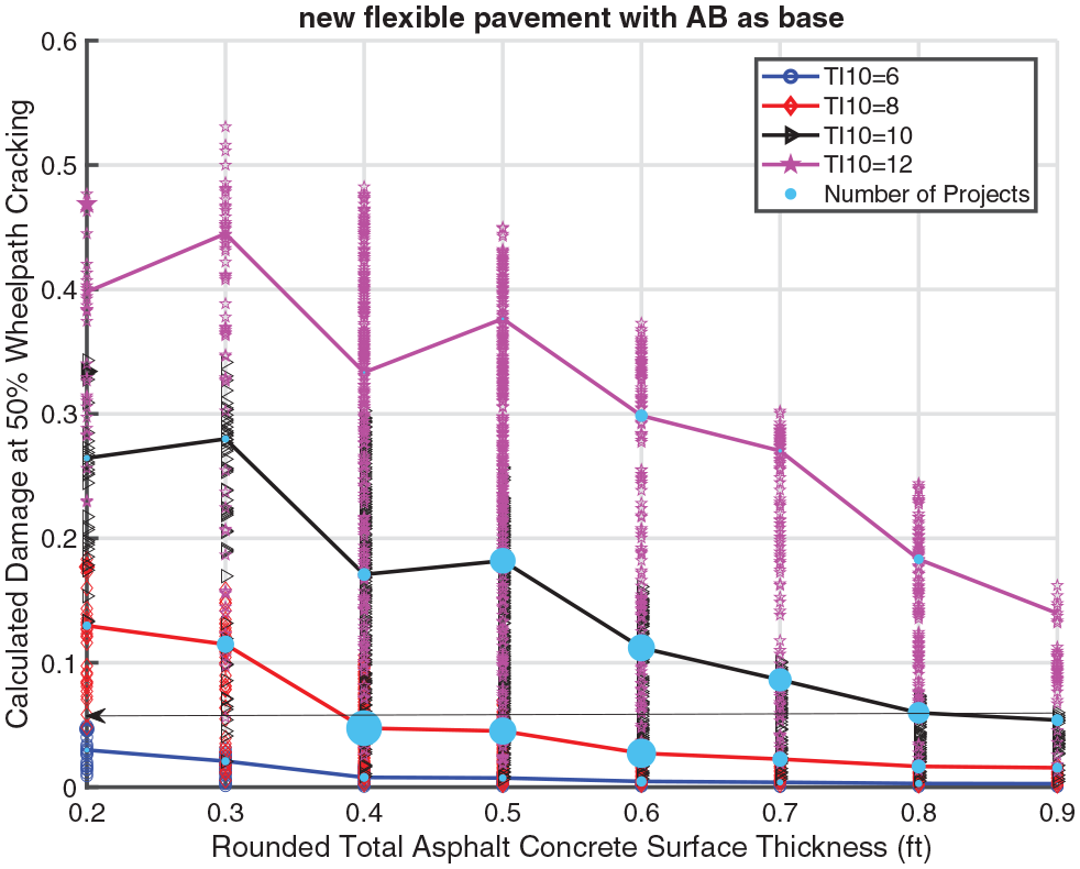
Determination of critical damage ${\mathit{\omega }}_{50}$ (i.e., the damage corresponding to 50% cracking), TI10 is a function of the estimated equivalent single axle loads applied in 10 years.

As shown in Figure 11, the values of ${\omega }_{50}$ (y-axis) were determined for each AC thickness and each assumed traffic volume (indicated by TI10). The size of the large solid circles indicates the amount of data with recorded TI10 that matches the assumed value. If the recorded TI10 values were accurate, the ${\omega }_{50}$ for each AC thickness with the largest solid circles should be used. Given that TI10 were only approximates, the calibrated ${\omega }_{50}$ was only required to approximately pass through the solid circles. For this calibration, a constant value of 0.06 was selected for ${\omega }_{50}$ , as indicated by the arrow in the plot, because it was approximately near the center of gravity of the circles. This process can be mathematically done by a weighted averaging process.

Selection of Shape Parameter $\mathrm{\beta }$

The distribution of the observed shape parameters for this calibration is shown in Figure 12, in which the CDFs are grouped by total AC layer thickness. The shape parameter $\beta$ is determined by reviewing the distribution of the observed shape parameter ${\beta }_{\mathrm{observed}}$ . Based on Figure 12, the most extreme values of the observed shape parameter ${\beta }_{\mathrm{observed}}$ is approximately −30. This value was selected for the transfer as a starting point to assess the contributions of the variability of mechanistic inputs to WPV.

Figure 12.

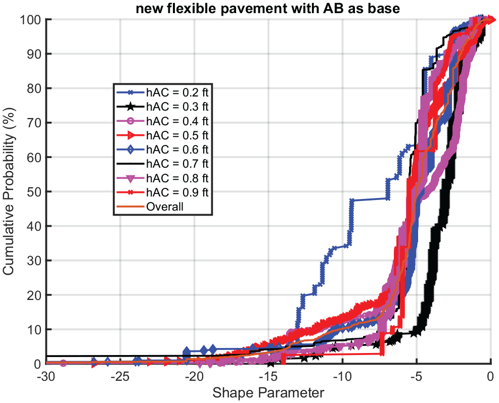
Distribution of observed shape parameter ${\mathit{\beta }}_{\mathrm{observed}}$ for each asphalt concrete (AC) surface thickness.

Determination of Within-Project Variability

As shown in Figure 12, the observed shape parameter ${\beta }_{\mathrm{observed}}$ has a wide range of values between −30 and 0. It was decided to use its median value, which is about −5.0, to represent the WPV.

The next step is to back-calculate the variance of selected M-E inputs that would result in the observed shape parameter. In CalME, WPV with respect to wheel path cracking performance is accounted for by sampling from the distributions of these three sets of variables for each layer:

• Thicknesses

• Stiffnesses

• Fatigue resistance

Distributions for each of these were available from previous research. A batch of Monte Carlo simulations was run with different combinations of asphalt layer thickness, stiffness, and fatigue parameter A variabilities (variances of other layers were found to be insignificant) to evaluate whether the resulting equivalent shape factors were similar to the median observed shape parameter. Multiple combinations were found to meet the criterion. One of the combinations included variances similar to the typical variances previously found in the literature and was selected to represent the WPV for use in design:

• Thickness: follows a normal distribution with a coefficient of variance of 0.07

• Stiffness: follows a lognormal distribution with a standard deviation factor (SDF, defined as $e^{\mathrm{cov}\left(\ln \left(x\right)\right)}$ for random variable x) of 1.20

• Fatigue model parameter A: follows a lognormal distribution with an SDF value of 1.35

Accounting for Between-Project Variability

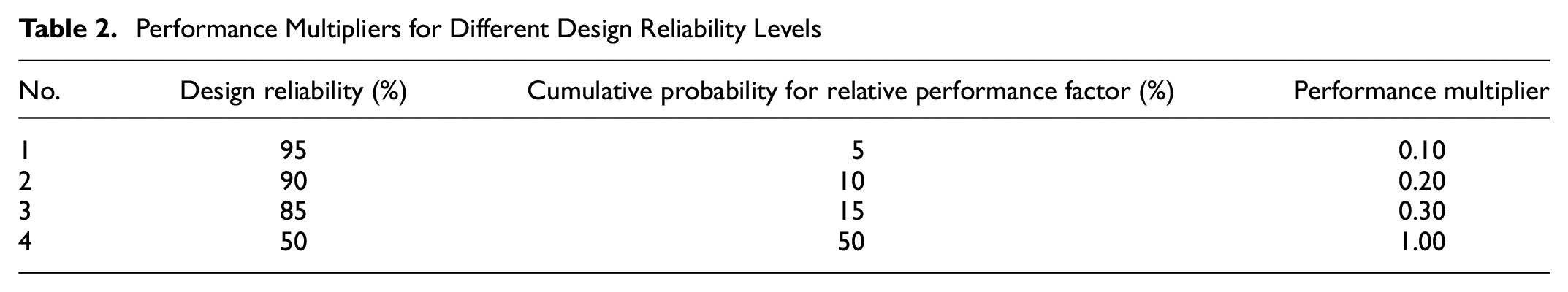
The cumulative distribution functions of the RPF for the N-AB sub-network are shown in Figure 13, which shows that the CDF functions of RPF for different AC surface thicknesses are generally similar. Therefore, it is believed that the overall CDF function can be used to account for the BPV.

Figure 13.

Distribution of relative performance factor for each asphalt concrete (AC) surface thickness.

The figure shows that the CDF function is roughly a straight line between (0, 0) and (1.0, 50%). Based on this observation, various performance multipliers were determined to account for BPV for different desired levels of design reliability. They are listed in Table 2. Note that these multipliers are applied to the $t_{50}$ predicted by CalME using the design NMI for each material to arrive at the design life for the given reliability level.

Table 2.

Performance Multipliers for Different Design Reliability Levels

No.	Design reliability (%)	Cumulative probability for relative performance factor (%)	Performance multiplier
1	95	5	0.10
2	90	10	0.20
3	85	15	0.30
4	50	50	1.00

Summary of the Calibration Results

A summary of the field calibration results is listed in Table 3. The WPVs for all sub-networks were found to be the same as those for the N-AB sub-network.

Table 3.

Summary of Calibration Results for Different Sub-Networks

Abbreviation	Critical damage ${\mathit{\omega }}_{50}$	Shape parameter $\mathit{\beta }$	Performance modifier for 95% reliability
N-AB	0.06	−30.0	0.10
N-CB	$0.0007·e^{0.0188*\mathrm{hAC}\_\mathrm{mm}}$ minimum 0.01, maximum 0.10	−90.0	0.23
R-FP	0.11	−90.0	0.20
R-RP	0.03	−90.0	0.20
R-PDR-EA	0.03	−30.0	0.10
R-FDR-FA	0.06	−30.0	0.32
R-FDR-C	0.03	−90.0	0.20

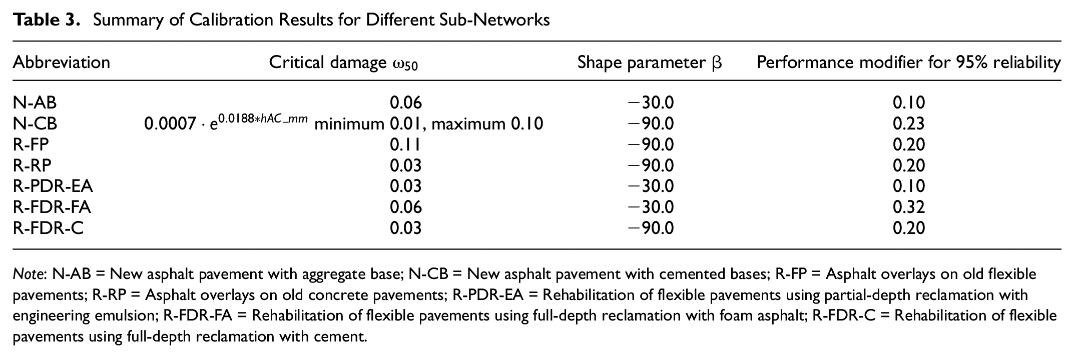
Note: N-AB = New asphalt pavement with aggregate base; N-CB = New asphalt pavement with cemented bases; R-FP = Asphalt overlays on old flexible pavements; R-RP = Asphalt overlays on old concrete pavements; R-PDR-EA = Rehabilitation of flexible pavements using partial-depth reclamation with engineering emulsion; R-FDR-FA = Rehabilitation of flexible pavements using full-depth reclamation with foam asphalt; R-FDR-C = Rehabilitation of flexible pavements using full-depth reclamation with cement.

Design With the Calibrated Model

To use the field-calibrated models for pavement design, a different set of statewide NMI for current materials, as opposed to historical periods, is needed to represent the condition of the pavements under design. These design NMI were determined by reviewing testing results from materials meeting current Caltrans specifications and practices. The underlying assumptions for using the field-calibrated models are that the transfer functions, and the BPVs and WPVs remain the same.

With the new approach for field calibration, CalME can accommodate the use of performance-related specifications (PRS) for AC mixes. This is achieved by using a larger performance modifier to account for the smaller BPV in PRS performance (BPV cannot be completely removed even with PRS).

Comparison With Empirical Design Results

As a check of reasonableness, the pavement designs produced by the calibrated fatigue cracking model were compared with the corresponding empirical designs.

The comparison showed that the two methods produce the same minimum HMA thickness when the design traffic volume is no higher about 1.0 million equivalent single axle loads (ESALs). CalME requires a greater HMA thickness as the design traffic increases than the empirical method. The difference increases as the design traffic volume increases. For example, for approximately 75 million design ESALs CalME with 95% design reliability and a new pavement designed for 5% wheel path cracking at the design life, requires 300 mm (1 ft) of HMA whereas the R-value method requires 225 mm (0.75 ft). This difference appears reasonable, considering unknown reliability of the R-value method, and that it was calibrated with a maximum of about 10 million ESALs.

Comparisons with the Pavement ME method are underway; space limitations do not permit their inclusion in this paper.

Summary and Conclusions

In this paper, a new approach for calibration of the transfer functions of M-E performance models and reliability calculations for design is proposed using “big data” from a PMS. The new approach is developed based on insights gained from simulated project- and network-level pavement performance data using the Monte Carlo method. In the new calibration approach, all M-E inputs are considered random variables with their own statistical distributions, separated into within-project and between-projects (i.e., within a network) variability.

The new approach can use network-level data from PMSs without requiring sampling and testing of materials from each project in the network. Instead, it requires knowledge of the statistical distributions of M-E design inputs over the network. The new approach also provides a basis for incorporating reliability in design for design-bid-build projects where the specific materials properties are not known at time of design, and where typical construction variability for a given material is known. The approach also considers differences between material input levels for historical projects used for calibration and materials used in current design.

The new approach is illustrated through the calibration of the cracking model for CalME, which is an M-E design method developed for the California Department of Transportation. The detailed steps, results, and considerations needed for the calibration are explained. The calibrated version of CalME is then compared against the empirical design method used by Caltrans. CalME was found to produce reasonable designs after calibration.

It is believed that the new field calibration approach is a breakthrough in M-E design development theory in relation to better integrating pavement design and management and understanding and accounting for sources of variability in calibration and design, although there are details that will certainly require further improvement, for example, how to handle an imperfect model.

Although not done as part of this study, it would be helpful to conduct field calibrations using both the proposed new approach and the approach outlined by AASHTO ( 4 ) and compare the results when data are available.