Sage Journals: Discover world-class research

Abstract

In-vehicle infotainment systems can increase cognitive load and impair driving performance. These effects can be alleviated through interfaces that can assess cognitive load and adapt accordingly. Eye-tracking and physiological measures that are sensitive to cognitive load, such as pupil diameter, gaze dispersion, heart rate (HR), and galvanic skin response (GSR), can enable cognitive load estimation. The advancement in cost-effective and nonintrusive sensors in wearable devices provides an opportunity to enhance driver state detection by fusing eye-tracking and physiological measures. As a preliminary investigation of the added benefits of utilizing physiological data along with eye-tracking data in driver cognitive load detection, this paper explores the performance of several machine learning models in classifying three levels of cognitive load imposed on 33 drivers in a driving simulator study: no external load, lower difficulty 1-back task, and higher difficulty 2-back task. We built five machine learning models, including k-nearest neighbor, support vector machine, feedforward neural network, recurrent neural network, and random forest (RF) on (1) eye-tracking data only, (2) HR and GSR, (3) eye-tracking and HR, (4) eye-tracking and GSR, and (5) eye-tracking, HR, and GSR. Although physiological data provided 1%–15% lower classification accuracies compared with eye-tracking data, adding physiological data to eye-tracking data increased model accuracies, with an RF classifier achieving 97.8% accuracy. GSR led to a larger boost in accuracy (29.3%) over HR (17.9%), with the combination of the two factors boosting accuracy by 34.5%. Overall, utilizing both physiological and eye-tracking measures shows promise for driver state detection applications.

Keywords

cognitive load estimation machine learning heart rate Galvanic skin response eye measures

Factors such as road environment (i.e., high traffic conditions), bad weather, and the usage of in-vehicle technologies (e.g., cellphones and infotainment systems) can increase the cognitive load experienced by drivers. Both simulator and on-road studies have shown that high cognitive load can impair driving performance and visual scanning behaviors (1, 2). Real-time assessment of cognitive load can enable vehicle manufacturers to provide preventative warnings and develop adaptive interfaces that can support drivers, for example, by actively limiting functionality on menu interfaces ( 3 ) and automatically filtering information when high levels of cognitive load is detected ( 4 ). Automated vehicle systems can also utilize cognitive load estimates to intelligently transfer vehicle control to the driver ( 5 ).

As summarized in Table 1, a variety of measures were found to be responsive to varying levels of external cognitive load experienced by drivers, including: (i) eye-tracking measures, such as pupil diameter (2, 6), blink rate ( 7 ), and standard deviation (SD) of horizontal gaze position (7, 8); (ii) physiological measures, such as heart rate (HR) (8 –10), galvanic skin response (GSR) (8, 9), and electroencephalography (EEG) (11, 12); (iii) driving performance measures, such as vehicle speed ( 8 ); and (iv) subjective measures, such as NASA-Task Load Index (NASA-TLX) ( 1 ).

Table 1.

Example Cognitive Load Measurements

Measure	Trend with increased cognitive taskload
Eye-tracking
Pupil diameter	↑ (2, 6)
Blink	Rate ↑ ( 7 )
Gaze position	Periphery/mirror/instrument check rate ↓ ( 1 )
	SD of horizontal position ↓ (7, 8)
	SD of vertical position ↓ ( 7 )
Physiological
HR	HR ↑ (8 –10)
	HR variability ↓ ( 10 )
GSR	↑ (8, 9)
EEG	Power of alpha band ↓ (11, 12)
	P300 latency ↑ ( 13 )
Respiration	Rate ↑ ( 9 )
Performance-based
Vehicle speed	Average ↑ ( 9 ) ↓ ( 8 )
	SD ↑ ( 9 ) ↓ ( 8 )
Steering wheel	Reversal rate ↑ ( 8 )
Subjective
NASA-TLX	↑ ( 1 )

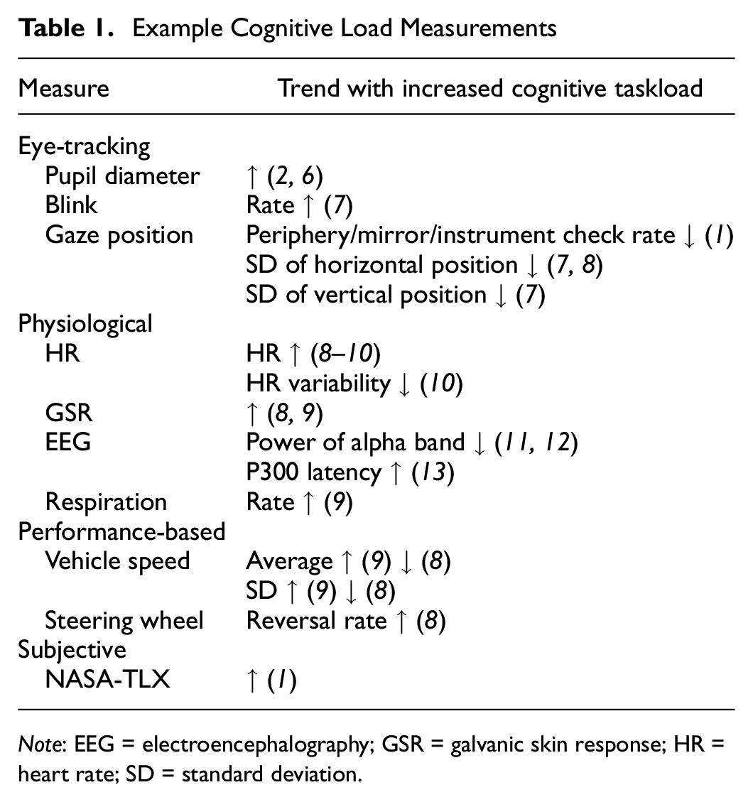
Note: EEG = electroencephalography; GSR = galvanic skin response; HR = heart rate; SD = standard deviation.

It is widely acknowledged that no single measure alone can provide sufficient information to estimate cognitive load (9, 11). Indeed, multiple measures have been combined in previous research to estimate the cognitive load experienced by drivers. For example, Solovey et al. ( 14 ) reached 89% accuracy in classifying 2 levels of cognitive load (no-task versus an auditory recall 2-back task) using driving performance, GSR, and HR data collected in an on-road study. Liang et al. ( 15 ) reached 81.1% accuracy in identifying 2 levels of cognitive load (no-task versus an auditory stock ticker task) using driving performance and eye-tracking data collected in a simulator study. In general, driving performance measures used in these earlier studies (e.g., speed and lane position) are highly sensitive to traffic conditions and may require additional driving context-assessment to improve their utility in driver state detection ( 16 ). This need for additional information can be a barrier for the use of driving performance measures in driver state detection.

The fusion of eye-tracking and physiological measures seems to be more promising for real-time assessment of driver cognitive load, yet research is lacking in this area. Eye-tracking measures have been adopted in several production cars for detecting visual distraction (e.g., Cadillac [ 17 ]) and drowsiness (e.g., Khan and Lee [ 18 ]). They have not yet been adopted for cognitive load detection, although pupil diameter (e.g., Recarte and Nunes [2, 6]), blink rate (e.g., Liang and Lee [ 7 ]), and gaze dispersion (e.g., Liang and Lee [ 7 ], Mehler et al. [ 8 ]) are known to be sensitive to cognitive load variation. Physiological measures, such as HR (e.g., Mehler et al. [8, 9], Brookhuis et al. [ 10 ]) and GSR (e.g., Mehler et al. [8, 9]), also react well to variations in cognitive demand and can now be collected through cost-effective and nonintrusive sensors, for example, in wearable devices such as the Apple Watch ( 19 ) and FitBit ( 20 ). Thus, combining eye-tracking with HR and GSR data is now a feasible solution for in-car applications, yet it is unknown what level of performance enhancement this combination may provide in driver cognitive load detection.

Using a dataset collected in a driving simulator study, this paper investigates the benefits of fusing eye-tracking and physiological data for driver cognitive load classification. It is hypothesized that increasing the number of features in the dataset by fusing different measure types would improve classification performance. In the simulator study, three levels of cognitive load (no external load, 1-back task, and 2-back task) were imposed by an audio-verbal cognitive task, the modified n-back task ( 21 ), while participants drove through an urban environment. A variety of machine learning methods used in earlier studies were explored on this three-class driver state estimation problem, including k-nearest neighbor (KNN, e.g., Solovey et al. [ 14 ]), support vector machine (SVM, e.g., Wang et al. [ 22 ]), feedforward neural network (FNN, e.g., Solovey et al. [ 14 ]), recurrent neural network (RNN, e.g., Shimizu et al. [23]), and random forest (RF, e.g., Barua et al. [ 24 ]). The models were built and compared using the following measures to investigate the benefits of fusing eye-tracking and different physiological data (in particular, HR and GSR):

• eye-tracking data only, including eye closure (i.e., fraction of the iris covered by the upper and lower eye lid), pupil diameter, and gaze rotation angle (i.e., the orientation of the eye gaze with respect to the world coordinate system);

• physiological data only, including HR and GSR;

• eye-tracking data and HR combined;

• eye-tracking data and GSR combined;

• eye-tracking data, HR, and GSR combined.

Data Source

The data utilized in this paper was collected from 33 participants in a driving simulator study originally reported by He et al. (21, 25), which investigated the effects of different levels of external cognitive demand on drivers’ physiological, eye-tracking, and driving performance. In a within subject design, participants completed three counterbalanced conditions (in three drives total): no external task, and two difficulty levels of an external cognitive task (i.e., a secondary task). Eye-tracking measures, including the level of eye closure, pupil diameter, and gaze rotation angle, as well as physiological measures, including Electrocardiography (ECG) and GSR, were collected. In the following, we provide an overview of the experimental methods, but a more detailed description of the methods can be found in He et al. ( 21 ). He et al. ( 26 ) also utilized physiological measures from this dataset for a preliminary machine learning application, but only with relatively simple machine learning models and without using eye-tracking data.

Participants

A total of 33 drivers (18 males and 15 females), recruited through campus and online posts, completed this driving simulator study. Participants were required to drive at least several times per month, to hold a full driver’s license (G license in Ontario, Canada or equivalent) for at least 3 years, and to be under 35 years old (average age: 27.6; SD: 4.45). The compensation was C$12 per hour, and the participants were told that they could receive a bonus of up to C$14 based on their secondary task performance as an incentive for engaging in the secondary task.

Apparatus

The study was conducted on a NADS miniSim™ driving simulator (Figure 1a). This fixed-based simulator has three 42-inch screens, creating a 130° horizontal and 24° vertical field at a 48-inch viewing distance. The center screen displays the left and center parts of the windshield; the right screen displays the rest of the windshield, the rear-view mirror, and the right-side window and mirror, whereas the left screen displays the left-side window and mirror.

Figure 1.

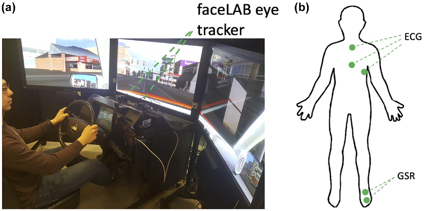
Apparatus: (a) driving simulator, the NADS miniSim and faceLAB 5.0 eye-tracking system and (b) placement of ECG and GSR sensors.

The eye-tracking information was collected at 60 Hz by using the faceLAB 5.0, a dashboard mounted eye-tracker by Seeing Machines. ECG was collected with three solid gel foam electrodes placed on participants’ chest; and GSR was collected with one solid gel foam electrode beneath the bare left foot and the other under the heel (Figure 1b). Both ECG and GSR sensors were from Becker Meditec and the data was collected at 240 Hz using the D-Lab software developed by Ergoneers.

Experimental Tasks

The secondary task used in this study was a modified version of an auditory-verbal n-back task widely used in driving research (e.g., Mehler et al. [8, 9]), and was validated to impose graded levels of cognitive load on drivers (21, 25). The modification was performed to minimize physiological signal interference because of speech. In each n-back task, participants listened to a prerecorded series of 10 letters, separated by approximately 2.5-second intervals, for an overall duration of approximately 25 s. For the 1-back task (lower cognitive load), participants were asked to silently count the number of times two identical letters appeared back-to-back (e.g., PP). For the 2-back task (higher cognitive load), participants were asked to silently count the number of times two identical letters appeared in pairs separated by one letter in between (e.g., DTD). Participants were asked to verbally provide their answer at the end of each n-back task. Figure 2 offers examples of auditory input provided to participants with the target instances highlighted with different colors.

Figure 2.

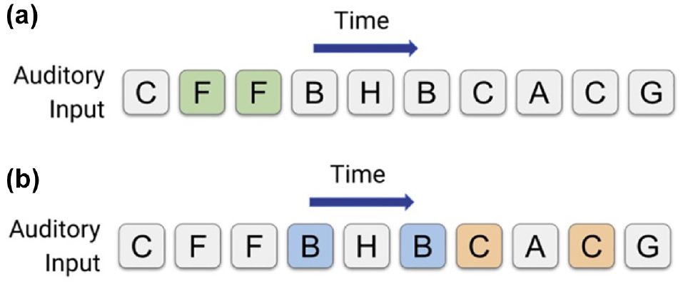
Visualization of the modified n-back task: (a) example 1-back task, the correct answer is “1” and (b) example 2-back task, the correct answer is “2.”

The driving scenarios were designed to involve mainly operational driving, without tactical decisions (e.g., navigation or passing a vehicle). Participants were asked to follow a lead vehicle at a speed of 40 mph (around 64.4 km/h) and a comfortable headway on a 4-lane urban road. In addition to training drives, each participant completed three driving tasks with different levels of the modified n-back task: baseline with no task, lower cognitive load with 1-back task, and higher cognitive load with 2-back task. The order of these three taskload levels was counterbalanced across participants. For machine learning models presented in this paper, data from four n-back tasks (a series of 10 letters for each n-back task) per drive were utilized. Participants had completed another two n-back tasks in each drive, but these corresponded to lead vehicle braking event response, which could affect physiological measures and was deemed to be outside the scope of the current analysis. In each n-back drive, the participants spent 100 s performing the four n-back tasks. This 100-s period for each n-back drive (i.e., 1-back and 2-back) and a corresponding 100-s period for the no-task drive were used in model building, leading to 300 s of data per participant being used in the machine learning models.

Procedures

After verifying their eligibility, participants were asked to sign a consent form. All participants completed a practice drive that was identical to the route used in the three experimental driving tasks. Participants were then provided written and oral instructions on the modified n-back task and practiced it without driving to ensure that they fully understood the secondary task. The eye-tracking system was then calibrated and the physiological sensors were placed on participants. Then, participants completed another practice drive while performing the secondary task. Participants went on to complete the three experimental driving tasks (no-task, 1-back, and 2-back).

Data Processing and Model Training

A three-class classification problem was pursued in our analysis: no-task versus 1-back task versus 2-back task. We fitted KNN, SVM, FNN, RNN, and RF models to different combinations of eye-tracking and physiological data. Overall, five different datasets were created as described in the following section.

Signal Processing and Feature Extraction

Table 2 summarizes our signal processing steps. In total, two physiological features were generated (HR and GSR) along with six eye-tracking features, including eye closure (EC) raw data, blink duration (BD), blink frequency (BF), pupil diameter (PD), eyeball rotation speed (eyeRS), and percentage of time at least 75% of iris is covered by eyelids (PERCLOS). These features were selected based on previous studies, which showed relationships between BF, PD, gaze dispersion and cognitive load, as summarized in Table 1. In place of SD of gaze position and periphery/mirror/instrument check rate reported in Table 1, we used eyeRS, which captures gaze dispersion and can be calculated independently of the driving scene (e.g., extracted through video of driver’s face only). Although no clear relationship has been found between BD and cognitive load (e.g., Tsai et al. [ 27 ]) and PERCLOS is primarily a measure of drowsiness (e.g., Khan and Lee [ 18 ]), we opted to include these features, as they can be readily available from eye closure data. All eye-tracking features were calculated for each eye and were then averaged across the two eyes.

Table 2.

Processing of Eye-Tracking and Physiological Measures to Obtain Machine Learning Features (i.e., Inputs)

Type	Measure	Features	Processing steps
EYE-TRACKINGSampled at 60 Hz	Eye closure (left and right): The fraction of the iris covered by the upper and lower eye lids (0: fully open to 1: fully closed)	4 features at 60 HzEC: eye closure raw dataBD: blink duration (ms)BF: blink frequency (number/second)PERCLOS: % of time at least 75% of iris is covered by upper and lower eyelids	(1) Identify frames with eye closure over 75% and frames with eye fully closed (for left and right eye separately)(2) For each eye, calculate average BD and PERCLOS within a window size of 10 s and step size of 1/60 s (i.e., 60 Hz)(3) For each eye, calculate the interblink intervals (intervals between two eye closures) and convert them into BF within a window size of 10 s and step size of 1/60 s(4) Average each feature across the two eyes
	Pupil diameter (left and right)	1 feature at 60 HzPD: pupil diameter (mm)	(1) Calculate average PD across the two eyes
	Gaze rotation angle (left and right): The orientation change of eyeball with respect to the world coordinate system, horizontally and vertically (rad)	1 feature at 60 HzeyeRS: eyeball rotation speed (rad/sec)	(1) For each eye, calculate the eyeball rotation angle for each data point, that is, the root-sum square of the horizontal and the vertical gaze rotation angles(2) Calculate average eyeRS (sum of eyeball rotation angles over the 10 s time window/10 s) with a window size of 10 s and a step size of 1/60 s(3) Average the feature across the two eyes
PHYSIOLOGICALSampled at 240 Hz	ECG	1 feature at 60 HzHR (/min)	(1) Remove polynomial trend of raw ECG data using the polyval function in MATLAB and identify R-peaks of detrended ECG using the findpeaks function ( 28 )(2) Calculate the average interbeat interval (ibi) with a window size of 5 s with a step size of 1/60 s(3) Convert ibi to HR
PHYSIOLOGICALSampled at 240 Hz	GSR	1 feature at 60 HzGSR (μSiemens)	(1) Calculate the average GSR every 1/60 s (i.e., 60 Hz)

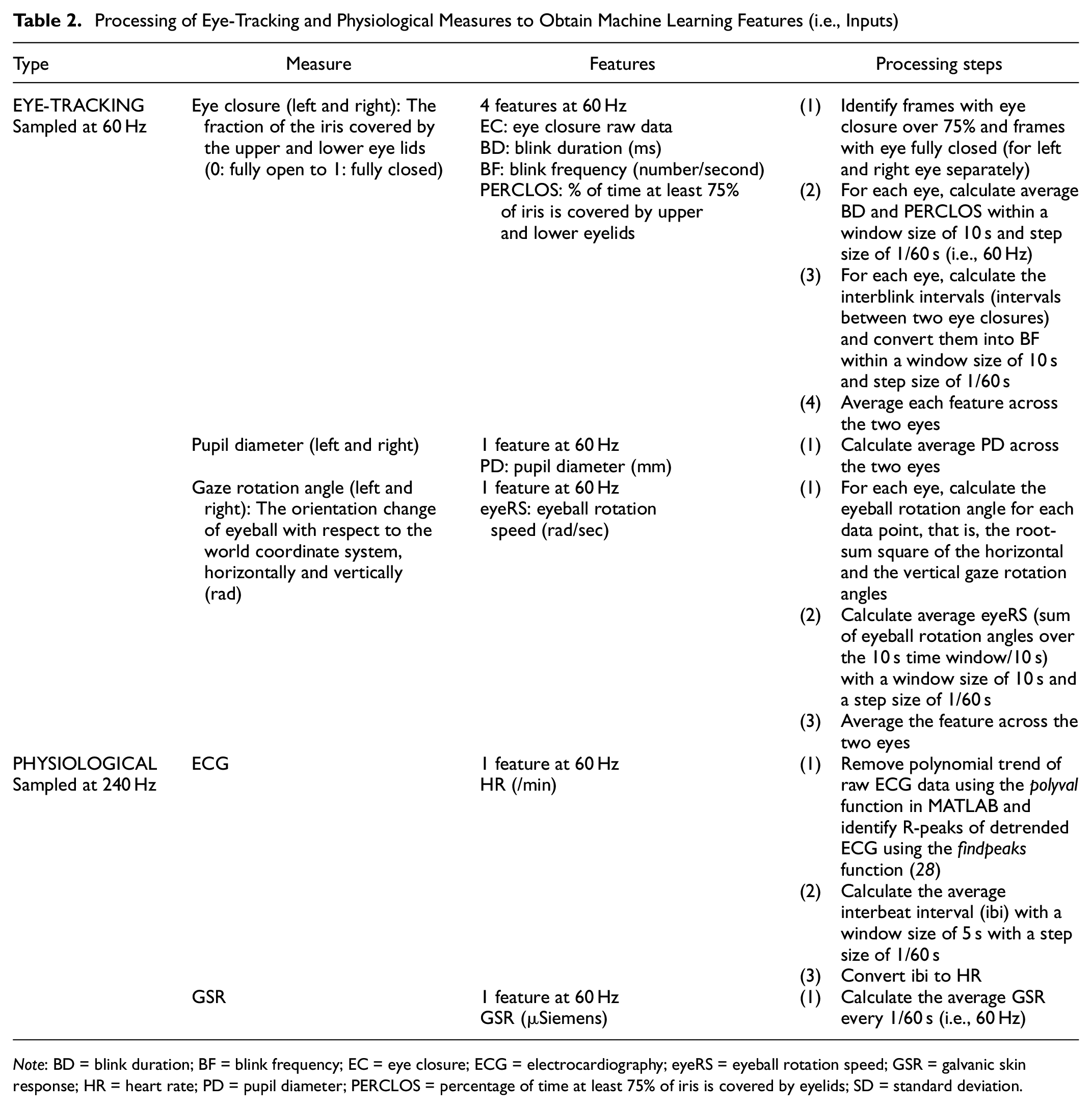
Note: BD = blink duration; BF = blink frequency; EC = eye closure; ECG = electrocardiography; eyeRS = eyeball rotation speed; GSR = galvanic skin response; HR = heart rate; PD = pupil diameter; PERCLOS = percentage of time at least 75% of iris is covered by eyelids; SD = standard deviation.

The measures that were originally sampled at a rate higher than 60 Hz (i.e., physiological measures) were downsampled to 60 Hz in order have equal number of data points across all features. All features, except EC, GSR, and PD, were calculated within a moving window. With a step size of 1/60 s (i.e., 60 Hz), a window size of 10 s was used for the eye-tracking features and a window size of 5 s was used for HR. The ECG data is noisy and, thus, is commonly converted into interbeat interval (ibi) data after R-peak detection (e.g., Solovey et al. [ 14 ]) and a running window procedure is necessary for this conversion. The 5-s window was adopted for HR based on our preliminary work on the same data investigating cognitive load detection ( 26 ). A longer time window was deemed necessary for eye-tracking measures given that, for example, the average blink frequency was recorded to be around 10 times/minute in De Padova et al. ( 29 ) and 24 times/minute in our dataset. Thus, a 10-s window size was chosen to provide a long enough period for reliable eye-tracking data extraction, but not too long compared with the entire data extraction period for each level of cognitive load (100 s), although earlier research used a longer time window for PERCLOS (30 s in Cardone et al. [ 30 ] and 1 min in Rodríguez-Ibáñez et al. [ 31 ]).

All features were extracted at 60 Hz leading to 594,000 rows of data (sampling frequency of 60 Hz × 25 s of data for each n-back task × 4 n-back tasks in each drive × 3 drives per participant × 33 participants). We built five datasets to train and evaluate our machine learning models:

• eyeSet, with eye-tracking features only;

• physioSet, with HR and GSR;

• eyeHRset, with eye-tracking features and HR;

• eyeGSRset, with eye-tracking features and GSR;

• eyePhysioSet, with all features.

Data Partition

As shown in Figure 3, a within-driver data partition approach was adopted, aiming to represent all participants in the training, validation, and test datasets. This data partition was selected over a between-drivers data partition method (which allocates some participants to the test dataset and the remaining to the training dataset), as we did not have a large enough sample to capture individual differences across participants that would be required for a between-drivers data partition. Hyperparameters were tuned using a 10-fold cross-validation on 90% of the data from each cognitive load level from each participant. The last 10% of the data from each level of cognitive load from each participant was used as the test dataset. Ten different splits (see Figure 3) were generated for the 10-fold cross-validation, each for one fold, with the training conducted on 81% of the data and the validation on 9%. A random split of training and test datasets was not appropriate for this data given its temporal nature and the resulting correlation over time.

Figure 3.

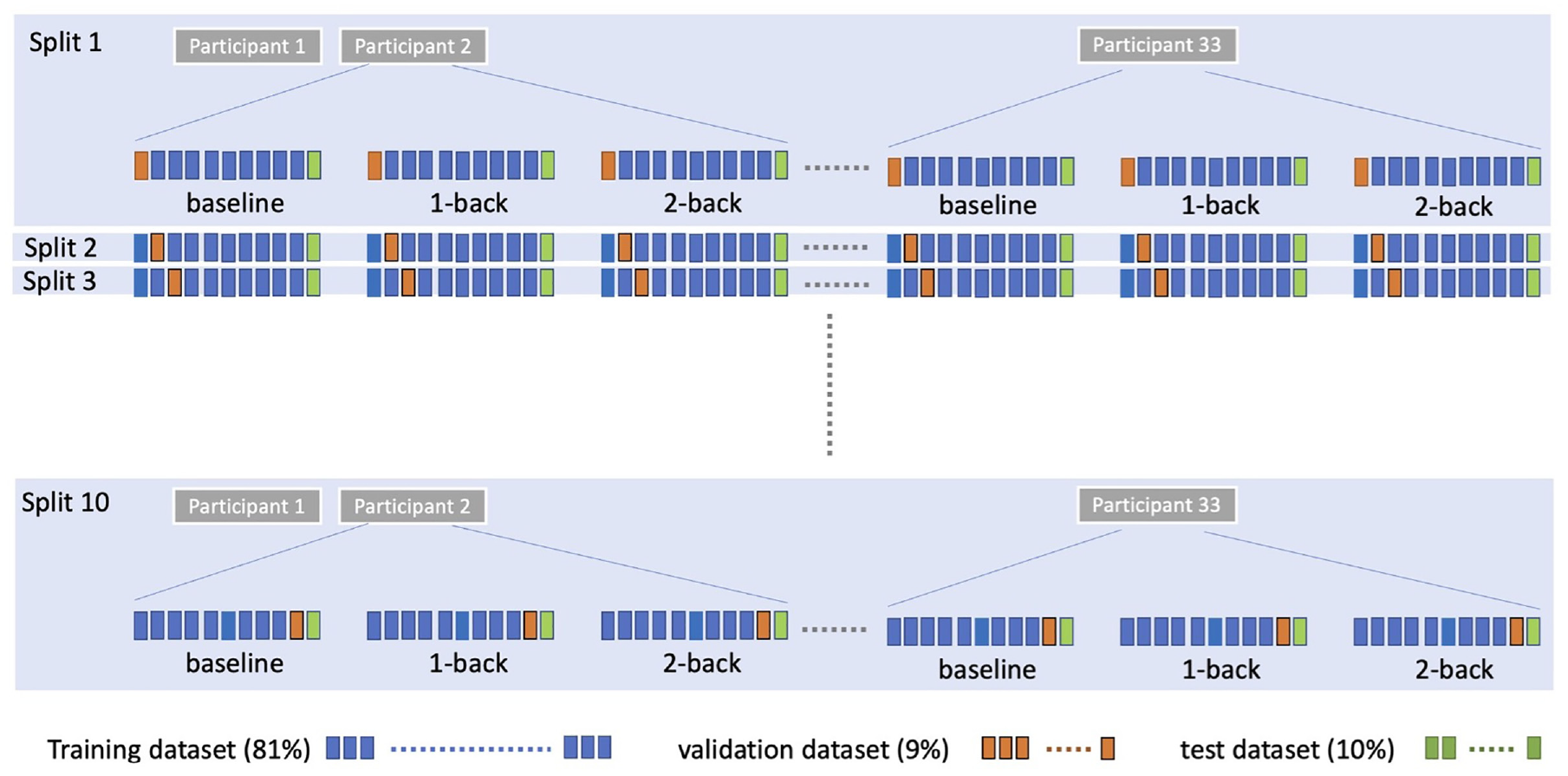
Visualization of data splits for cross-validation and testing. Note that the boxes are arranged to fall on a timeline for each cognitive load level and represent 10 s of data (with 100 s for each level of cognitive load and 300 s in total for each participant). Each blue and orange box represents 9% (i.e., 540 consecutive samples) and each green box represents 10% (i.e., 600 consecutive samples) of the total samples for each cognitive load level for each participant.

Data Preparation

Previous work has shown that individual differences among drivers influence the accuracy of driver state classification when eye-tracking and physiological data are used (32, 33). To minimize this effect, each participant’s data were normalized with respect to their no-task responses in the training dataset as

X_{score} = \frac{X_{raw} - {\bar{X}}_{notask}}{S_{notask}}

(1)

where $X_{score}$ = normalized feature value; $X_{raw}$ = raw feature value; and ${\bar{X}}_{notask}$ and $S_{notask}$ = mean and standard deviation of that feature for the no-task condition in the training dataset.

Further, each feature was also standardized using the scale of the features from the training dataset. Data standardization can control for scale differences across features and has been shown to improve the overall model accuracy in models such as KNN ( 34 ) and neural networks ( 35 ). Feature standardization was performed as in

X_{scaled} = \frac{X_{score} - {\bar{X}}_{training}}{S_{training}}

(2)

where $X_{scaled}$ = standardized feature score; $X_{score}$ = normalized feature score in Equation (1); and ${\bar{X}}_{training}$ and $S_{training}$ = mean and the standard deviation of the feature in the training dataset.

Model Training

All machine learning models were built in Python. Modules from the Scikit-Learn Library ( 36 ) were used to train and test SVM, FNN, KNN, and RF, whereas Keras ( 37 ) was used for RNN. The specific functions used are documented in Table 3. Hyperparameters were tuned through a grid-search approach using cross-validation (i.e., iterating over combinations of parameters and selecting those that resulted in the highest average accuracy on validation datasets). All models were trained on an Apple MacBook Pro (16 in., 2019) with 2.6 GHz 6-Core Intel i7 CPU and 16 GB 2667 MHz DDR4 RAM. Graphical processing units were not used in the training of the neural network models.

Table 3.

Overview of Model Fitting and Hyperparameters Explored. The Best Combinations of Hyperparameters for Each Model are Indicated With the Following Superscripts: ^eeyeSet, ^pphysioSet, ^eheyeHRset, ^egeyeGSRset, ^epeyePhysioSet

Model	Functions and candidate hyperparameters
KNN	Function: KNeighborsClassifier from Scikit-Learn libraryNumber of Neighbors: 1, 2^{[e, p, eh, ep]}, 3, 4^[eg], 5, 6, 7, 8, 9, 10Weight Function: uniform, distance ^{[e, p, eh, eg, ep]}Distance Metric: Euclidean, Manhattan ^{[e, p, eh, eg, ep]}
SVM	Function: svm.SVC from Scikit-Learn libraryKernel (fixed): RBF ^{[e, p, eh, eg, ep]}Regularization Parameter: 50.0^[eh], 100.0^{[e, p, eg, ep]}Kernel Coefficient:1^{[e, p, eh, eg, ep]}, 0.1
FNN	Function: MLPClassifier from Scikit-Learn libraryArchitecture (number of neurons in each hidden layer): 2-8, 8-32, 16-64, 2-4-2, 8-16-8, 32-64-32, 2-4-8-4, 8-16-32-16, 16-32-64-32^{[e, p, eh, eg, ep]}Minibatch Size (fixed): 50^{[e, p, eh, eg, ep]}Activation Function: tanh^{[e, p, eh, eg, ep]}, ReLULearning Rate: constant at 0.001 ^{[eh, eg]}, adaptive (initialized at 0.001) ^{[e, p, ep]}Regularization Rate for L2 Penalty: 0.001, 0.01^{[e, p, eh, eg, ep]}
RNN	Function: Sequential from Keras libraryBatch Size: 32, 64^{[e, p, eh, eg, ep]}, 128Sliding Window (window-overlap): 6-3, 8-4^{[e, p, eh, eg, ep]}, 10-5, 20-10Learning Rate: 0.01, 0.001^{[e, p, ep]}, 0.0001 ^{[eh, eg]}Architecture: • 1^st LSTM layer ○ Dimensionality of the output space: 32-512 ○ Activation function (fixed): tanh^{[e, p, eh, eg, ep]} ○ Whether to return the last state in addition to the output: True ^{[e, p, eh, eg, ep]} • Dropout layer: ○ Drop rate: 0-0.3 • 2^nd LSTM layer ○ Dimensionality of output space: 32-512 ○ Activation function (fixed): tanh^{[e, p, eh, eg, ep]} ○ Whether to return the last state in addition to the output: False ^{[e, p, eh, eg, ep]} • Dropout layer: ○ Input units to drop: optimal value between 0-0.3 • 1^st to n^th (n: 1^{[p, eh]}, 2^[eg], 3^[ep], 4^[e], 5) dense layer, each followed with one dropout layer ○ Dimensionality of output space: 32-512 ○ Activation function: ReLU, tanh, Sigmoid ○ Drop rate: 0-0.3 • Last dense layer: ○ Activation function (fixed): Softmax^{[e, p, eh, eg, ep]}
RF	Function: RandomForestClassifier from Scikit-Learn libraryNumber of Trees in the Forest: 5, 10, 20, 30, 50, 100 ^{[e, p, eh, eg, ep]}Function to Measure the Quality of a Split (fixed): Gini impurity ^{[e, p, eh, eg, ep]}Bootstrap or Not: True ^{[e, p, eh, eg, ep]}, False

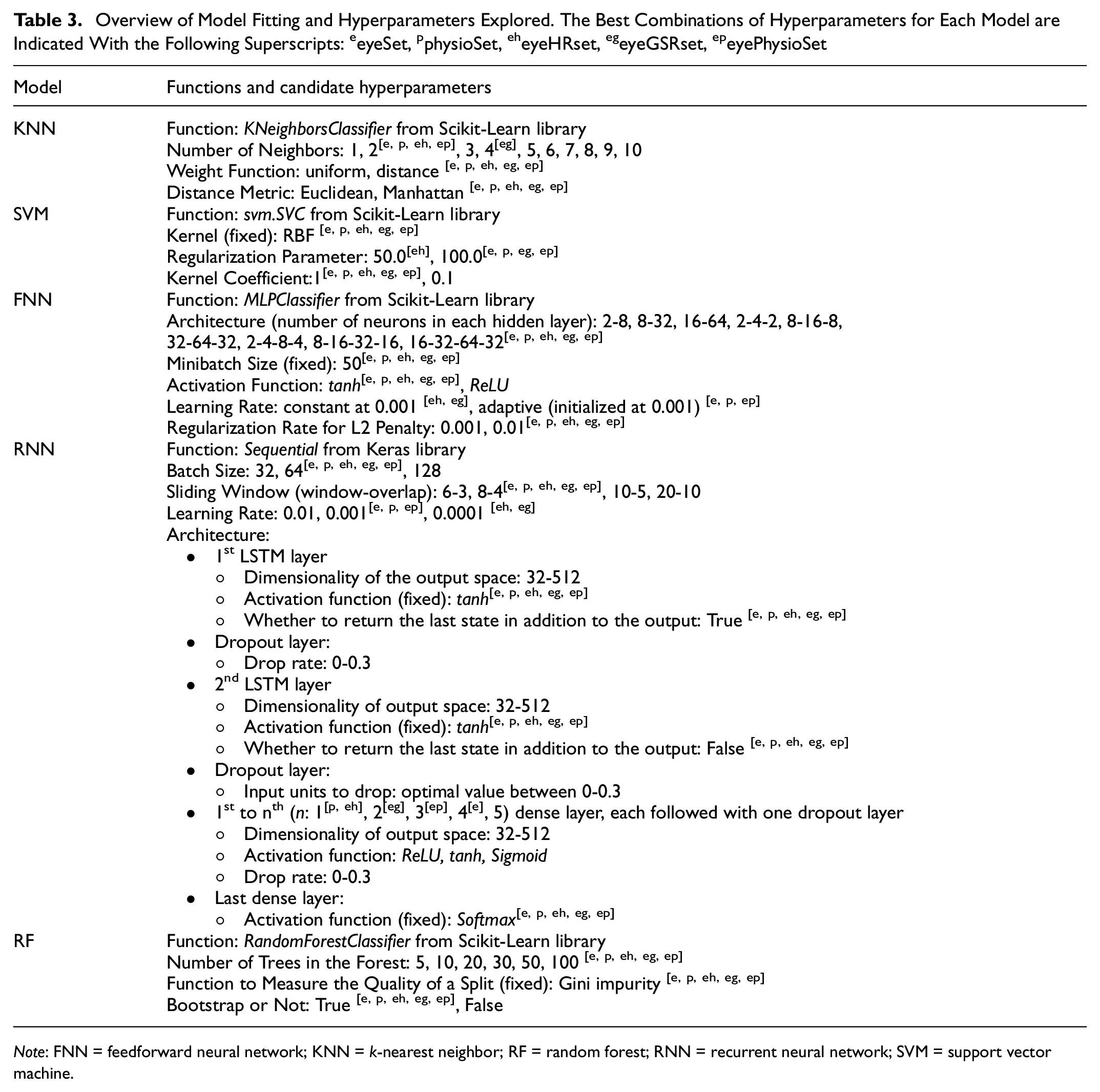
Note: FNN = feedforward neural network; KNN = k-nearest neighbor; RF = random forest; RNN = recurrent neural network; SVM = support vector machine.

Table 3 summarizes the candidate hyperparameters we tested and the best for each dataset and for each machine learning model. For KNN, the number of neighbors specifies the number of training data samples that can vote for the prediction of a given test data point. The weight function dictates how the voting samples are weighted. The distance metric dictates how the distances between the unknown sample and the voting samples are calculated. For SVM, a radial basis function (RBF) kernel was used, as it yielded the best performance in most of the previous attempts in classifying levels of cognitive load with SVM (e.g., Liang et al. [ 15 ], Wang et al. [ 22 ], He et al. [ 26 ]). Two additional hyperparameters were tuned for SVM. The regularization parameter trades off model complexity for training accuracy and the kernel coefficient defines how far the influence of a single training example reaches ( 36 ). For FNN, the activation function defines the (nonlinear) output of the neuron in the network given a set of inputs, the learning rate controls how quickly the model is adapted to the problem and the L2 regularization rate decides how much the model is regularized to reduce the likelihood of overfitting.

Traditional RNNs may suffer from the exploding or vanishing gradient problems, that is, if the input sequence is too long, the RNN model might be unstable (38, 39). A long short-term memory (LSTM) architecture solves this problem by adding three gates to the network (40, 41), and has been found to perform well in time-sequence classification ( 42 ). For this reason, we used LSTM in our RNN architecture. Further, the use of a sliding window has been shown to improve the performance of neural networks for time-series prediction ( 43 ). Thus, we explored several combinations of moving window size and step size. Our RNN consisted of two LSTM layers, each followed by a dropout layer, which prevents the model from overfitting by randomly setting the input units to 0. The dropout rate defines the frequency of the input units being ignored (i.e., set to 0). Then, 1 to 5 layers of fully connected layers were used, each followed by a dropout layer as well. The last fully connected layer outputs the classification of the estimated cognitive load into one of the three classes. For RF, if bootstrap is true, the whole dataset is used to build each tree; otherwise, bootstrap samples are used when building trees, which means a subset of the samples was used for the training of each tree.

Results

Figure 4 shows the classification accuracy on the test dataset for each machine learning model for the different combinations of features. Figure 5 provides confusion matrices on the test dataset. The average accuracies on cross-validation were comparable to the test accuracies and, thus, are not reported; this indicates that overfitting or underfitting are unlikely to have occurred.

Figure 4.

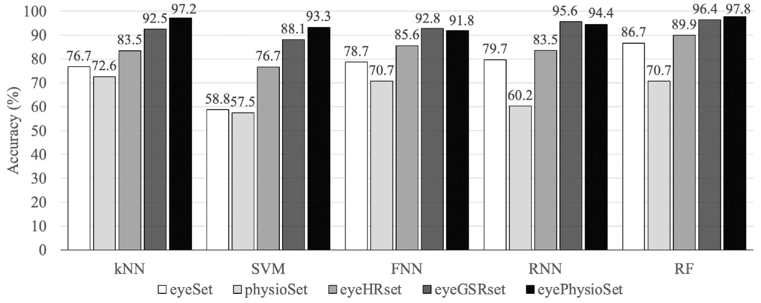
Classification accuracies in identifying three levels of cognitive load on test dataset.

Figure 5.

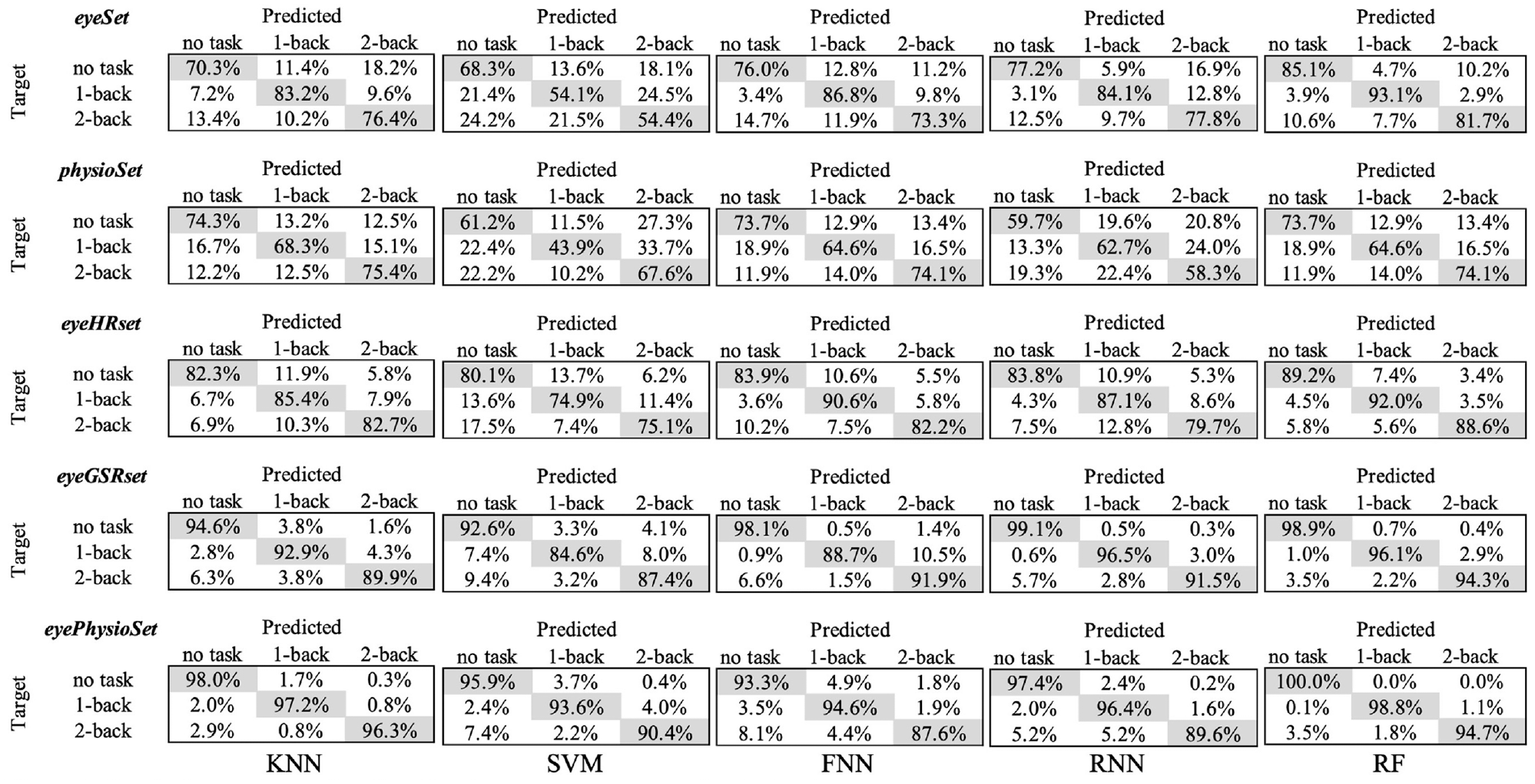
Confusion matrices for classification performance on the test dataset.

It can be observed that RF generated the highest prediction accuracy (97.8%) when all eye-tracking and physiological features were used (eyePhysioSet data). Although using physiological features alone (physioSet) generated worse prediction accuracy (1%–15%) compared with using eye-tracking features alone (eyeSet), adding physiological features in addition to eye-tracking features increased the model prediction accuracies. Among the physiological features, GSR seems to have provided more predictive power compared with HR. When comparisons are made across machine learning models, it can be seen that the discrepancies between different models decreased with the expansion of the feature set. The confusion matrices indicate that different models may be good at identifying different levels of cognitive load, even if the models may be comparable in relation to their overall accuracy. For example, with all features utilized, RF was better at differentiating no task from 1-back task (i.e., lower level of cognitive load) compared with KNN, but KNN was better at differentiating 1-back task from 2-back task (i.e., higher level of cognitive load).

Discussion

This paper revealed the potential for improving cognitive load estimation through combining eye-tracking and physiological measures. Eye-tracking measures are being adopted in production vehicles for distraction (e.g., Cadillac [ 17 ]) and drowsiness (e.g., Khan and Lee [ 18 ]) detection, but also hold promise for cognitive load detection (e.g., Recarte and Nunes [2, 6], Liang and Lee [ 7 ]). Further, physiological measures are also promising for cognitive load detection: earlier studies that used physiological predictors to classify drivers’ cognitive load reported classification accuracies of 85%–96% (14, 22, 26, 44). However, not all physiological measures are suitable for driver state estimation because of the intrusiveness of associated sensors (e.g., EEG). Further, although the fusion of eye-tracking and physiological measures seems to be more promising for real-time assessment of driver cognitive load, research is lacking in this area.

In this paper, two physiological measures that are available in consumer-grade wearable devices, that is HR and GSR, were fused with eye-tracking measures, leading to 97.8% accuracy with a RF model in classifying three levels of cognitive load (no task, lower difficulty 1-back task, and higher difficulty 2-back task). This result is promising when compared with the accuracies reached in previous research that combined driving performance with eye-tracking measures (e.g., 81.1% in Liang et al. [ 15 ]), and also with the accuracies reached in previous research that combined driving performance measures with physiological measures (e.g., 89% in Solovey et al. [ 14 ]), especially considering that our 3-class classification problem is more challenging than the 2-class problems tackled in these earlier studies. GSR contributed more to the performance of the models compared with HR: when HR was added to eye-tracking data, the model accuracies increased from 3.2% (with RF) to 17.9% (with SVM), whereas with HR, the increases ranged from 9.7% (with RF) to 29.3% (with SVM). Although adding both HR and GSR to eye-tracking data yielded the highest accuracies for most models, the benefit of adding HR on top of GSR was relatively small, with changes in model accuracies ranging from −1.2% (with RNN) to 5.2% (with SVM). Collecting and processing more features may come with monetary and computational costs, and if a choice is to be made, GSR may be preferred over HR.

Our findings reveal that, with the increased number of features, the advantage of using a specific machine learning model becomes less obvious. With only eye-tracking measures, RF yielded the highest accuracy (86.7%) and SVM the lowest (58.8%). When both eye-tracking and physiological measures were used, all models reached over 91% accuracy. It is possible that with more features, the classification problem became easy enough for most models to handle. At the same time, we also note that KNN, which yielded the second highest accuracy (97.2%) on the combined eye-tracking/physiological dataset, took the shortest to train with 7.6 s, and RF, which resulted in the highest accuracy (97.8%), took slightly longer with 61.6 s. The training time for FNN, RNN, and SVM were two orders of magnitude longer (all over 5000s) than that of KNN and RF. Thus, even with the computation cost of model training considered, RF and KNN are preferred over other models for the cognitive load detection problem explored in our study.

Although overall accuracies across models were comparable when all features were utilized, the confusion matrices reveal that different models may be good at identifying different levels of cognitive load. For example, when all features were utilized, RF reached the overall highest accuracy, but KNN performed better than RF in differentiating 2-back from 1-back. Thus, the choice of models may not be based solely on overall accuracies, but also on the specific purpose of the in-vehicle applications, for example, which level of cognitive load is most critical to differentiate from other levels for an alert to be issued.

Individual differences among drivers have been shown to affect the accuracy of driver state classification based on physiological data ( 32 ) and, thus, we used a normalization strategy, which would require the system to have prior data from each driver, or learn from the driver over time. This is a reasonable expectation but prior data may not always be available for each driver. Future research should utilize a larger sample with a more diverse set of drivers to test the generalization of our models by training the models based on a group of participants and predicting the cognitive load of a different group of participants (i.e., between-drivers data partition). It should, however, be noted that if model training/testing is based on a between-drivers data partition, individual differences would have a greater effect on model performance.

Further, although we utilized a validated secondary task to impose cognitive workload on our participants, the task is artificial and there is a need to study more the tasks that drivers normally perform in their vehicles (e.g., talking on a cellphone). In addition, in this paper, we focused on physiological measures (i.e., HR and GSR) that can be collected through wearable devices, but our data came from a research-grade system utilized in a driving simulator study. Further, the eye-tracking measures were collected using an eye-tracker built for the laboratory environment. There are bound to be additional signal noise issues when these measures are collected through wearable devices and cameras, and in a real vehicle. Although our study provided evidence that HR and GSR have the potential to be fused with eye-tracking data to improve driver cognitive load estimation, more research is needed to develop signal processing algorithms for relevant data collected through consumer-grade wearable devices in motion and through in-vehicle eye-tracking systems under varying lighting conditions. As in Fuller et al. ( 45 ), Zhu and Du ( 46 ), and Binaee et al. ( 47 ), there is indeed significant research activity to improve these devices and accompanying algorithms. Finally, the time window sizes used for feature extraction may affect the performance of the models. Future research should explore different time window sizes appropriate for this application.

In summary, physiological and eye-tracking features that can be collected through in-vehicle or wearable devices combined with the algorithms developed in our paper have the potential to support less intrusive driver state detection. Given that our approach excluded driving performance measures, it can also inform driver state detection for automated vehicles where driving performance data may not be indicative of driver state.

Footnotes

Author Contributions

The authors confirm contribution to the paper as follows: study conception and design: D. He, B. Donmez; analysis and interpretation of results: D. He, Z. Wang, E. B. Khalil, B. Donmez, and G. Qiao; draft manuscript preparation: D. He, E. B. Khalil, B. Donmez, Z. Wang, and S. Kumar. All authors reviewed the results and approved the final version of the manuscript.

Declaration of Conflicting Interests

The author(s) declared no potential conflicts of interest with respect to the research, authorship, and/or publication of this article.

Funding

The author(s) disclosed receipt of the following financial support for the research, authorship, and/or publication of this article: The funding for this study was provided by the Natural Sciences and Engineering Research Council of Canada (NSERC) through the Discovery Grant Program [RGPIN-2016-05580] and Hitachi Solutions, Ltd. through a research contract.

ORCID iDs

Dengbo He

Elias B. Khalil

Birsen Donmez

Shekhar Kumar

Data Accessibility Statement

Data sharing is not applicable to this article as no new data were created in this study.

References

Harbluk

J. L.

Noy

Y. I.

Trbovich

P. L.

Eizenman

An On-Road Assessment of Cognitive Distraction: Impacts on Drivers’ Visual Behavior and Braking Performance. Accident Analysis & Prevention, Vol. 39, No. 2, 2007, pp. 372–379.

Recarte

M. A.

Nunes

L. M.

Effects of Verbal and Spatial-Imagery Tasks on Eye Fixations While Driving. Journal of Experimental Psychology: Applied, Vol. 6, No. 1, 2000, p. 31.

Rogers

Fiechter

C. -N.

Thompson

Adaptive User Interfaces for Automotive Environments. Proc., IEEE Intelligent Vehicles Symposium 2000, Dearborn, MI, IEEE, 2000.

Strayer

D. L.

Cooper

J. M.

Turrill

Coleman

J. R.

Hopman

R. J.

The Smartphone and the Driver’s Cognitive Workload: A Comparison of Apple, Google, and Microsoft’s Intelligent Personal Assistants. Canadian Journal of Experimental Psychology/Revue canadienne de psychologie expérimentale, Vol. 71, No. 2, 2017, p. 93.

Johns

Sibi

Effect of Cognitive Load in Autonomous Vehicles on Driver Performance During Transfer of Control. Proc., 6th International Conference on Automotive User Interfaces and Interactive Vehicular Applications, Association for Computing Machinery, New York, NY, 2014.

Recarte

M. A.

Nunes

L. M.

Mental Workload While Driving: Effects on Visual Search, Discrimination, and Decision Making. Journal of Experimental Psychology: Applied, Vol. 9, No. 2, 2003, p. 119.

Liang

Lee

J. D.

Combining Cognitive and Visual Distraction: Less Than the Sum of its Parts. Accident Analysis & Prevention, Vol. 42, No. 3, 2010, pp. 881–990.

Mehler

Reimer

Coughlin

J. F.

Sensitivity of Physiological Measures for Detecting Systematic Variations in Cognitive Demand From a Working Memory Task: An On-Road Study Across Three Age Groups. Human Factors: Journal of Human Factors and Ergonomics Society, Vol. 54, No. 3, 2012, pp. 396–412.

Mehler

Reimer

Coughlin

J. F.

Dusek

J. A.

Impact of Incremental Increases In Cognitive Workload on Physiological Arousal and Performance In Young Adult Drivers. Transportation Research Record: Journal of the Transportation Research Board, 2009. 2138: 6–12.

10.

Brookhuis

K. A.

de Vries

De Waard

The Effects of Mobile Telephoning on Driving Performance. Accident Analysis & Prevention, Vol. 23, No. 4, 1991, pp. 309–316.

11.

Ryu

Myung

Evaluation of Mental Workload with A Combined Measure Based On Physiological Indices During a Dual Task of Tracking and Mental Arithmetic. International Journal of Industrial Ergonomics, Vol. 35, No. 11, 2005, pp. 991–1009.

12.

Borghini

Astolfi

Vecchiato

Mattia

Babiloni

Measuring Neurophysiological Signals in Aircraft Pilots and Car Drivers for the Assessment of Mental Workload, Fatigue and Drowsiness. Neuroscience and Biobehavioral Reviews, Vol. 44, 2014, pp. 58–75.

13.

Strayer

D. L.

Turrill

Cooper

J. M.

Coleman

J. R.

Medeiros-Ward

Biondi

Assessing Cognitive Distraction in the Automobile. Human Factors: Journal of Human Factors and Ergonomics Society, Vol. 57, No. 8, 2015, pp. 1300–1324.

14.

Solovey

E. T.

Zec

Garcia Perez

E. A.

Reimer

Mehler

Classifying Driver Workload Using Physiological and Driving Performance Data. Proc., 32nd Annual ACM Conference on Human Factors in Computing Systems - CHI ‘14, Toronto, ON, Canada, 2014.

15.

Liang

Reyes

M. L.

Lee

J. D.

Real-Time Detection of Driver Cognitive Distraction Using Support Vector Machines. IEEE Transactions on Intelligent Transportation Systems, Vol. 8, 2007, pp. 340–350.

16.

Miller

Literature Review Workload Measures. Report No.: N01-006. National Advanced Driving Simulator, Iowa City, 2001.

17.

Cadillac. Super Cruise - Hands Free Driving. Cadilac Ownership. 2021. https://www.cadillac.com/world-of-cadillac/innovation/super-cruise.

18.

Khan

M. Q.

Lee

A Comprehensive Survey of Driving Monitoring and Assistance Systems. Sensors, Vol. 19, No. 11, 2019, p. 2574.

19.

Apple. The Future of Health is on Your Wrist. https://www.apple.com/ca/watch/.

20.

Fitbit. Understand Your Stress So You Can Manage It. https://www.fitbit.com/global/us/technology/stress.

21.

Donmez

Liu

C. C.

Plataniotis

K. N.

High Cognitive Load Assessment in Drivers Through Wireless Electroencephalography and the Validation of A Modified n-Back Task. IEEE Transactions on Human-Machine Systems, Vol. 49, No. 4, 2019, pp. 362–371.

22.

Wang

Y. K.

Jung

T. P.

Lin

C. T.

EEG-Based Attention Tracking During Distracted Driving. IEEE Transactions on Neural Systems and Rehabilitation Engineering, Vol. 23, No. 6, 2015, pp. 1085–1094.

23.

Shimizu

Shima

Mukaeda

Muraji

Matsuo

Horiue

Real-Time Evaluation of Driver Cognitive Loads Based on Multivariate Biosignal Analysis. Proc., IEEE International Conference on Systems, Man, and Cybernetics (SMC), Toronto, ON, Canada, IEEE, 2020.

24.

Barua

Ahmed

M. U.

Begum

Towards Intelligent Data Analytics: A Case Study in Driver Cognitive Load Classification. Brain Sciences, Vol. 10, No. 8, 2020, p. 526.

25.

Liu

C. C.

Donmez

Plataniotis

K. N.

Assessing High Cognitive Load in Drivers Through Electroencephalography. Proc., Transportation Research Board 96th Annual Meeting (17-02615), Washington, D.C., 2017.

26.

Risteska

Donmez

Chen

Driver Mental Workload Classification Through the Use of Physiological Data. In Digital Signal Processing and Machine Learning for Interactive Systems Developers ( Eslambolchilar

Komninos

Dunlop

, eds.), Association for Computing Machinery, New York, NY, 2021.

27.

Tsai

Y. -F.

Viirre

Strychacz

Chase

Jung

T. -P.

Task Performance and Eye Activity: Predicting Behavior Relating to Cognitive Workload. Aviation, Space, and Environmental Medicine, Vol. 78, No. 5, 2007, pp. B176–B185.

28.

MathWorks. R Wave Detection in the ECG. https://www.mathworks.com/help/wavelet/ug/r-wave-detection-in-the-ecg.html.

29.

De Padova

Barbato

Conte

Ficca

Diurnal Variation of Spontaneous Eye Blink Rate in the Elderly and its Relationships With Sleepiness and Arousal. Neuroscience Letters, Vol. 463, No. 1, 2009, pp. 40–43.

30.

Cardone

Filippini

Mancini

Pomante

Tritto

Nocco

Perpetuini

Merla

Driver Drowsiness Evaluation by Means of Thermal Infrared Imaging: Preliminary Results. Proc., Infrared Sensors, Devices, and Applications XI, San Diego, 2021.

31.

Rodríguez-Ibáñez

García-González

M. A.

Fernández-Chimeno

Ramos-Castro

Drowsiness Detection by Thoracic Effort Signal Analysis in Real Driving Environments. Proc., 2011 Annual International Conference of the IEEE Engineering in Medicine and Biology Society, Boston, IEEE, 2011.

32.

Lin

C-. T.

R-. C.

Liang

S-. F.

Chao

W-. H.

Chen

Y-. J.

Jung

T-. P.

EEG-Based Drowsiness Estimation for Safety Driving Using Independent Component Analysis. IEEE Transactions on Circuits and Systems I: Regular Papers, Vol. 52, No. 12, 2005, pp. 2726–2738.

33.

Jin

Jiang

Xian

Gao

Effects of Driver Behavior Style Differences and Individual Differences on Driver Sleepiness Detection. Advances in Mechanical Engineering, Vol. 7, No. 4, 2015, p. 1687814015578354.

34.

Peterson

L. E.

K-Nearest Neighbor. Scholarpedia, Vol. 4, No. 2, 2009, p. 1883.

35.

Shanker

M. Y.

Hung

M. S.

Effect of Data Standardization on Neural Network Training. Omega, Vol. 24, No. 4, 1996, pp. 385–397.

36.

Pedregosa

Varoquaux

Gramfort

Michel

Thirion

Grisel

Blondel

Prettenhofer

Weiss

Dubourg

Vanderplas

Scikit-Learn: Machine Learning in Python. Journal of Machine Learning Research, Vol. 12, 2011, pp. 2825–2830.

37.

Chollet

Keras: The Python Deep Learning Library. Astrophysics Source Code Library, 2018.

38.

Pascanu

Mikolov

Bengio

On the Difficulty of Training Recurrent Neural Networks. Proc., International Conference on Machine Learning, Atlanta, 2013.

39.

Lipton

Z. C.

Berkowitz

Elkan

A Critical Review of Recurrent Neural Networks for Sequence Learning. arXiv Preprint arXiv:150600019, 2015.

40.

Greff

Srivastava

R. K.

Koutník

Steunebrink

B. R.

Schmidhuber

LSTM: A Search Space Odyssey. IEEE Transactions on Neural Networks and Learning Systems, Vol. 28, No. 10, 2016, pp. 2222–2232.

41.

Hochreiter

Schmidhuber

Long Short-Term Memory. Neural Computation, Vol. 9, No. 8, 1997, pp. 1735–1780.

42.

Wang

J-. H.

Liu

T-. W.

Luo

Wang

An LSTM Approach to Short Text Sentiment Classification With Word Embeddings. Proc., 30th Conference on Computational linguistics and Speech Processing (ROCLING 2018), Hsinchu, Taiwan, China, 2018.

43.

Frank

R. J.

Davey

Hunt

S. P.

Time Series Prediction and Neural Networks. Journal of Intelligent and Robotic Systems, Vol. 31, No. 1–3, 2001, pp. 91–103.

44.

Kohlmorgen

Dornhege

Braun

M. L.

Blankertz

Müller

K-. R.

Curio

Hagemann

Bruns

Schrauf

Kincses

W. E.

Improving Human Performance in a Real Operating Environment Through Real-Time Mental Workload Detection. In Toward Brain-Computer Interfacing ( Dornhege

Millan

J. d. R.

Hinterberger

McFarland

D. J.

Mller

K-. R.

, eds.), MIT Press, Cambridge, MA, 2007, pp. 409–422.

45.

Fuller

Colwell

Low

Orychock

Tobin

M. A.

Simango

Buote

, et al. Reliability and Validity of Commercially Available Wearable Devices for Measuring Steps, Energy Expenditure, and Heart Rate: Systematic Review. JMIR mHealth and uHealth, Vol. 8, No. 9, 2020, p. e18694.

46.

Zhu

Improved Heart Rate Tracking Using Multiple Wrist-Type Photoplethysmography During Physical Activities. Proc., 40th Annual International Conference of the IEEE Engineering in Medicine and Biology Society (EMBC), Honolulu, HI, IEEE, 2018.

47.

Binaee

Sinnott

Capurro

K. J.

MacNeilage

Lescroart

M. D.

Pupil Tracking Under Direct Sunlight. Proc., ACM Symposium on Eye Tracking Research and Applications, Germany, 2021.

Classification of Driver Cognitive Load: Exploring the Benefits of Fusing Eye-Tracking and Physiological Measures

Abstract

Keywords

Data Source

Participants

Apparatus

Experimental Tasks

Procedures

Data Processing and Model Training

Signal Processing and Feature Extraction

Data Partition

Data Preparation

Model Training

Results

Discussion

Footnotes

Author Contributions

Declaration of Conflicting Interests

Funding

ORCID iDs

Data Accessibility Statement

References