Sage Journals: Discover world-class research

Abstract

Long-term insight into maritime traffic is critical for port authorities, logistics companies, and port operators to proactively formulate suitable policies, develop strategic plans, allocate budget, and preserve and improve competitiveness. Forecasting freight rate is a spotlight in port traffic literature, but relatively little research has been directed at forecasting long-term vessel traffic trends. Based on forecast long-term freight rate input provided by the recent 10-year strategic planning of the port of Rajaee, the largest port of Iran, the paper implements seasonal autoregressive integrated moving average (SARIMA) and neural network (NN) models to forecast its container vessel traffic between 2020 and 2025. A database consisting of monthly container traffic data for this port from 1999 to 2019 is utilized. The comparison between the two forecasting models is fulfilled by benchmarking the naïve method. The results reveal the superiority of the NN model over SARIMA in this practice. Considering NN model outputs, the port should expect a significant increase in Panamax and Over-Panamax vessels in the future, and, if not timely addressed, this would result in a systemic queue in the port of Rajaee. That said, the approach can be implemented in port planning and design to avoid under- or over-estimations in such capital-intensive projects.

Keywords

artificial intelligence artificial intelligence and advanced computing applications container data analytics data and data science freight transportation data logistics machine learning (artificial intelligence)marine marine transportation (water transportation)neural networks port ports and channels vessels

A port master plan describes the required projects and provides an indicative measure for development phases. This long-term guide entails preliminary investigations, among which port traffic forecast plays an imperative role. As the main prerequisite in master planning, future maritime traffic specifies future vessel calls at specific times and supports the preparation of detailed steps based on the economic demand of the project ( 1 ).

To be more successful, all details must be carefully recorded for the brownfield while monitoring regional, national, and global changes (e.g., the amount of trade exchanged in the port’s hinterland, and cooperation and competition) to strengthen the forecast ( 2 ). Such information is then used to forecast the cargo throughput (demand study) in the short- and long-term, for example, Australian container ports, port of Hong Kong, major ports in India, container ports of South Africa, supply/demand relationship in Trinidad and Tobago, major Turkish container ports, and UK ports, to name but a few, with different methodologies (3 –9).

Although such long-term cargo traffic forecasts give an intuition about the vessel traffic, there are two limitations:

The results are limited, as throughput time series are expressed in tones, and they do not give any information about the number of vessels.

The results do not acquire any insight into the future, and they are limited to the data itself.

These limitations are addressed in this paper.

In this article, the long-term container vessel traffic at Rajaee port (with 80% share of Iran’s container throughput) is forecast using two methods. The seasonal autoregressive integrated moving average (SARIMA) model as a simple integrated approach is applied to the available dataset, as it has a good model fitting degree in decision-making ( 10 ). Also, as another method, the neural network (NN) model with simple components such as inputs, neurons or nodes, processing components, and outputs, interconnected with high forecasting capability, is applied to the dataset. Using NNs to forecast traffic behavior does not necessitate identifying mathematical functions to demonstrate the relationship between data, as artificial NNs recognize the inherent interactions between the data indicated by weights. A naïve method is used as a benchmark for comparing the performance of NN and SARIMA models ( 11 ).

The novelty of the proposed models lies in the use of linear and non-linear models to forecast future container traffic, which can aid port authorities in decision-making and strategic planning. Exploring the use of these three models in maritime traffic forecast, the forecasting models would be applicable in various realistic and theoretical cases related to maritime traffic.

Despite relatively widespread studies performed concerning port demand forecasting—short-term flow forecasting—less attention has been paid to marine long-term traffic forecasting of target ports, while there is an inevitable linkage between them. Therefore, this paper presents a methodology for long-term traffic forecast based on learning similar traffic patterns as a reference for forecasting future traffic. The main advantage of this approach is that the forecasts are generated based on the observed historical traffic patterns discovered from the historical datasets. The proposed methodology outperforms simple forecasting methods in relation to forecast accuracy, provided that enough samples are available in the archived datasets.

To the authors’ best knowledge, this study is the first attempt to apply NN and SARIMA models to forecast container ports maritime traffic.

In doing so, the next section unfolds the literature of maritime traffic forecasting approaches. The data, their preparation and filtering, and the categorization of vessels are discussed in the section after that. Then, the following section outlines the materials and method, detailing the NN model employed and its parameters together with the SARIMA model. The penultimate section presents the evaluation results and discusses the relevant research implications. The final section concludes the results of this research.

Literature Review

Short-term forecasts are usually used directly in daily port operations involving purchasing new machinery and materials, allocating and arranging workers, and modifying equipment ( 12 ). Most short-term forecasting research was performed using standard statistical methods such as simple smoothing, complex analyzes of time series, and filtering methods ( 13 ). In extrapolation and time series analysis, auto-regressive integrated moving average models (ARIMAs) are commonly used. Variations of the ARIMA model—such as the seasonal ARIMA (SARIMA) model—have also been implemented ( 14 ). These methods based on parametrization are not appropriate for unstable and complex marine traffic conditions. Non-parametric methods, such as methods relying on data analysis and NN methods, on the other hand, are mostly data-driven and apply empirical algorithms to projections. Such methods are advantageous as they are free from any assumptions concerning the definition of the underlying model and the uncertainty associated with estimating the model’s parameters. For instance, Wang and Shi forecast daily vessel traffic by defining four types of daily vessel traffic—including cargo ship, passenger ship, and tanker ship—and employed a hybrid technique in the forecast phase by combining autoregressive moving average (ARMA) and artificial neural network (ANN) to use their linear and non-linear strength ( 15 ).

Although short-term forecasting is appropriate for managing daily port operations, forecasting ports’ future activities is generally based on long-term rather than short-term forecasting ( 16 ). Also, its insight affects processes and procedures, for example, pricing and service quality, which call for appropriate benchmarking ( 17 ). Rather than planning an integrated strategy for maritime shipping, long-term forecasting of maritime traffic depends significantly on supply and demand. Excess demand causes rapid congestion in the port’s limited storage areas and decreases the supporting machines’ performance, further aggravating the problem. Limited supply not meeting the demands will increase vessel traffic and waiting times, requiring a new shipping line or bigger cargo volumes, resulting in a significant increase in the total costs or a gradual decrease in port calls ( 17 ).

Therefore, the absence of long-term plans for future traffic to create logical adjustment between demand and supply causes drastic contradictions between sophisticated maritime technology, facilities, and traffic management. In this case, vessel traffic flow forecasting provides a typical framework for long-term port planning that contains the development of facilities and the acquisition of heavy equipment to meet the long-term demand for port services ( 18 ). The problem is that traffic behavior’s complexity complicates the forecast of vessel traffic behavior because it depends on several factors, such as vessel type, production rate, operation type, and port layout. Therefore, mapping a mathematical relationship between factors that can support accurate traffic behavior forecasting is essential yet complicated ( 2 ).

Long-term throughput forecasts have a long history, and their tipping points are appreciated (17, 19 –23). Furthermore, some restrictions arise by forecasting throughput because the freight rate does not always represent economic activity. Besides, as the vessel traffic flow is non-linear, traditional forecasting methods—such as regression, time series, and grey theory—do not perform properly ( 24 ). Developing soft computing methods have played a significant role in modeling the complex non-linear relationships between variables affecting vessel traffic in recent years. In long-term traffic forecasting, regression analysis, support vector machines (SVMs), and NNs have been used in port planning projects in the past (21, 25, 26).

For example, Mostafa forecast maritime traffic flows in the Suez Canal using both univariate ARIMA and NN models in the long-term traffic forecast field ( 27 ). Their model with monthly net ton data provided useful insights into the behavior of maritime traffic. Yoo et al. forecast future vessel traffic of Busan port, Gwangyang port, and Incheon port by using a time series model, based on monthly converted traffic data from January 1996 to June 2013, to provide the necessary data for a port design and vessel traffic services (VTS) operation ( 28 ). Because of the model’s case-specific performance, each port was analyzed separately to diagnose the difference in monthly vessel traffic depending on the season. Panahi et al. mapped the marine traffic of four main container ports based on 17 years of recorded trade data based on three different situations: “simplified continuous development,”“offering replication for greatest experience,” and “regional best practices” ( 29 ).

Based on the above, the authors argue that most studies, including the above, have used forecasting models for freight rate forecasting. There is, however, no research on the application of the forecasting models for forecasting traffic. So, the aim of this research is to fill this gap.

Data

The dataset used in this research includes daily data of container vessels based on four inputs, including container service type and location, emptiness and fullness of vessels, and throughput resulting from the container vessels’ size. Descriptions about the categorization of container vessels’ size are addressed in Categorization of Vessels section.

Data Preparation

Two steps have been taken through this process: data filtering and categorization of vessels.

Data Filtering and Handling Missing Values

The process of reducing or eliminating the content of noises or errors from recorded data in any statistical analysis is known as “data filtration” and it improves the correctness of results by completing missing data and cutting outliers in data.

Correlations between deadweight tonnage (DWT), gross registered tonnage (GRT), or both, of specific vessel types and the main dimensions are commonly represented in standards and handbooks (29 –31). Since the DWT of vessels was not stated in some cases, it is calculated as a function of gross tonnage (GT). According to Overseas Coastal Area Development Institute (OCDI) for container vessels ( 30 ):

GT = 0.880 DWT

(1)

Moreover, outliers should be identified and avoided to cut the outliers in data in processing collected data, for instance, human errors (e.g., data entry errors) ( 32 ). As a result, the main dimensions of vessels are checked with an international source using their International Maritime Organization (IMO)’s number and name, and less than 0.1% of raw data was eliminated ( 33 ).

Categorization of Vessels

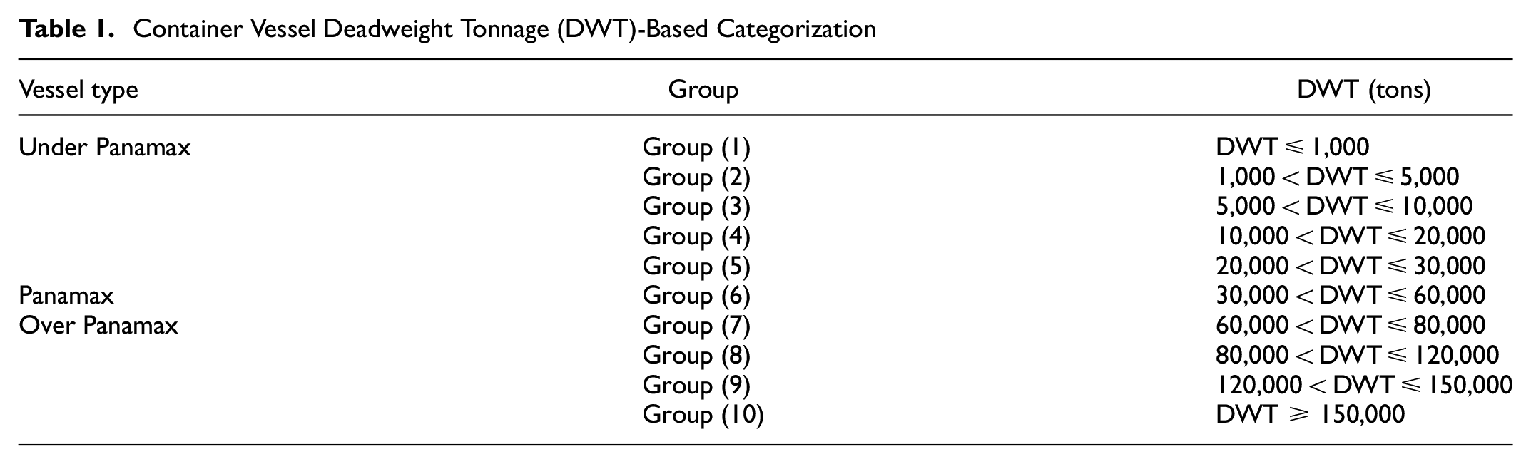
Containership capacity is generally expressed in twenty-foot equivalent units (TEUs). However, because of the incompleteness of recorded TEU data, in this study, containership data is categorized based on DWT ( 30 ). Both past and present container vessel patterns in the target port have been analyzed based on the containers’ size. On this account, 100,139 records of container vessels which called Rajaee port (such as the Japanese standard) between 1999 and 2019 have been categorized into 10 groups. They are selected in a way to have enough vessels in each group for preparing statistical calculations. According to OCDI, container vessels are classified into three groups: Under Panamax (small feeder, feeder, and feedermax), Panamax, and Over Panamax (Post Panamax, New Panamax, and Ultra Large Container Vessels [ULCV]) ( 30 ). Mentioned clustering is shown in Table 1:

Table 1.

Container Vessel Deadweight Tonnage (DWT)-Based Categorization

Vessel type	Group	DWT (tons)
Under Panamax	Group (1)	DWT ≤ 1,000
	Group (2)	1,000 < DWT ≤ 5,000
	Group (3)	5,000 < DWT ≤ 10,000
	Group (4)	10,000 < DWT ≤ 20,000
	Group (5)	20,000 < DWT ≤ 30,000
Panamax	Group (6)	30,000 < DWT ≤ 60,000
Over Panamax	Group (7)	60,000 < DWT ≤ 80,000
	Group (8)	80,000 < DWT ≤ 120,000
	Group (9)	120,000 < DWT ≤ 150,000
	Group (10)	DWT ≥ 150,000

Data Structure

The total throughput from 2020 through 2025 is reported by the Ports and Maritime Organization (PMO) of Iran based on the port’s historical data and capacity. The historical throughput of Rajaee container port and the future 6-year container traffic of Rajaee port as the focus of this paper is summarized in Figure 1. The port’s future throughput forecast in previous studies by PMO is used as future throughput for forecasting future inputs and outputs. The future forecasts of the port’s container capacity are used to forecast the investment needed to expand the port.

The volume of container operations in Rajaee port from 1999 to 2011 increased from 2.9 million tons in 1999 to 25.6 million tons in 2011. However, after that and until 2015, because of international sanctions against Iran, there was a declining trend, and then it re-acquired its ascending trend.

Emptiness and fullness of vessels is an effective parameter in container traffic for which the two parameters of the capacity of each container vessel and the ratio of the cargo carried by a vessel to its capacity are useful to analyze the current conditions of the port’s maritime traffic as well as forecasting its future traffic. The historical data revealed that, with the increase in container vessels’ capacity, the possibility of being full load has been reduced (Figure A.1, Supplemental Material).

Optimizing the loading and unloading time of containers in container terminals where containers must be transported by trucks between the vessel and the designated locations in the container area is an important issue. The speed of loading/unloading operations depends on the availability of cranes and trucks. The operation time should be reduced to approach maximum efficiency. Therefore, one of the critical parameters is the service type of the vessel. The historical data revealed that a major part of the container operations in Rajaee port is loading (Figure A.2, Supplemental Material). The share of loading and unloading operations in Rajaee port is assumed to remain similar to its trend from 1999 to 2019.

In the process of moving containers, the waiting time of the trucks in the area should be optimized to have a minimum need for sterile carriers with the possibility of parallel operation between the cranes. A significant part of the container operations is carried out through the Rajaee port’s yard (Figure A.3, Supplemental Material). So, it is necessary to create a suitable space for trucks and cranes. The share of non-stop and in-yard operation in Rajaee port is assumed to remain similar to its trend from 1999 to 2019.

Therefore, the dataset comprises 100,139 columns, and four rows—the vessels’ carriage tonnage, their emptiness and fullness percent, the vessels’ operation type, and the location—and is transferred to monthly records, which contains 252 columns and four rows to keep track of time monthly.

Figure 1.

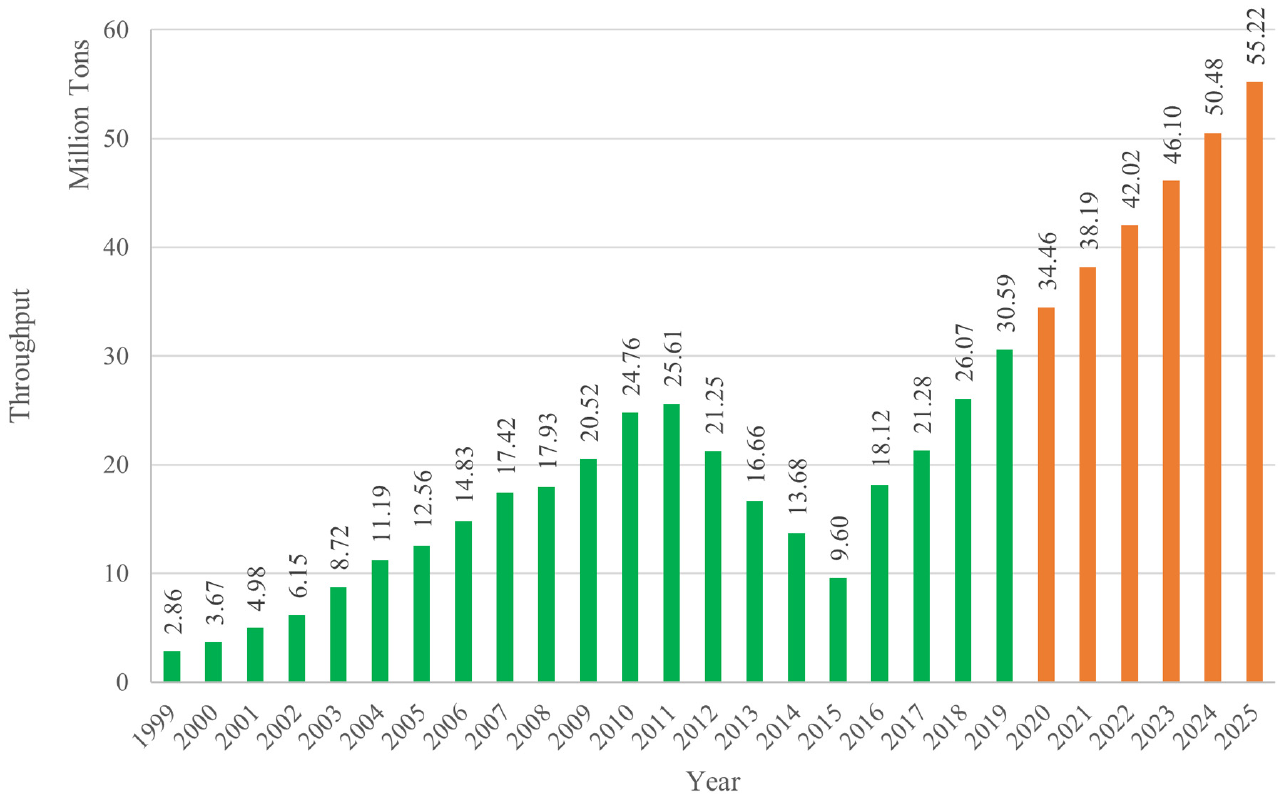
The (forecast) throughput of Rajaee container port, 1999–2025.

Method

In this study, two analysis methods have been used to forecast container traffic in Rajaee port from 2020 to 2025. A complete discussion of the proposed methodologies and formulations are presented Neural Network and ARIMA models in sections. Although “sophisticated” forecasting methods seem more precise, “naïve” forecasts can also be used as a safe benchmark ( 34 ). Therefore, a naïve forecast is performed with the naïve function to have a better insight into the subject.

The appropriate method is then selected and adopted based on the performance analysis according to a comparison between the forecast values against the recorded ones. In doing so, the mean square error (MSE) and the mean absolute scaled error (MASE) are calculated.

Neural Network (NN)

As a type of cause-and-effect model based on the human brain structure, NN is commonly used to forecast freight rates in the maritime field. Figure 2 shows the framework of the forecasting model.

Figure 2.

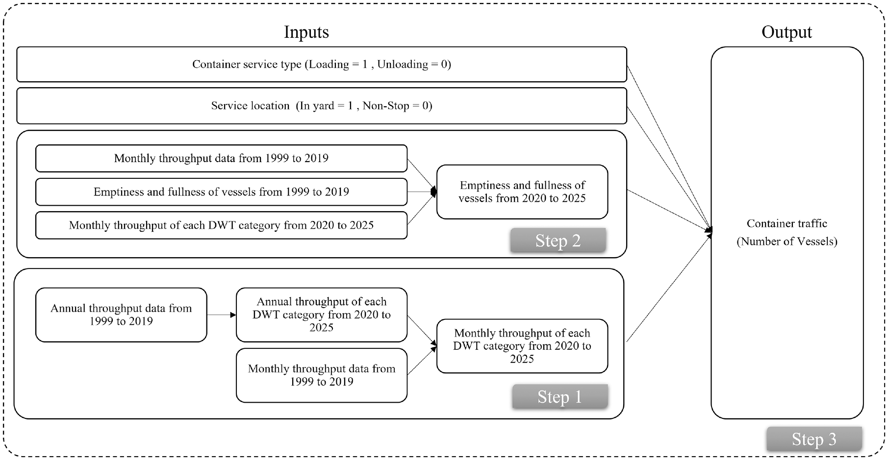
Framework of the forecasting model.

The primary step in NN models is data pre-processing. The outcomes of this phase are then the input values of the last phase.

Data Pre-Processing

The input data in NNs should be processed before using them. Although pre-processing is not necessary in many cases from the mathematical aspect, the NN training process would be enhanced. Using modified inputs in the network would result in a better match between real and forecast outputs ( 35 ). In general, both input and output vectors become normalized; therefore, the network outputs fall into a normalized range. It can be claimed that the NN stays on a structure between two pre-processing and post-processing steps.

In this study, pre/post-processing has been applied to input and output vectors, including remove-constant rows and min-max that respectively process the database by removing rows with constant values and converting the minimum and maximum row values to [−1 1].

In the min-max algorithm, it is assumed that variables have only finite real values; besides, all elements of each row are not equal.

Neural Network (NN) Structure

Based on the container market characteristics, the network structure of NN is specified, and multilayer perception neural network (MLP-NN), a dynamic network, is applied in this study to capture the container market’s characteristics. In a dynamic network, output depends on network inputs, as well as on previous inputs and outputs; accordingly, dynamic networks eventuate in more accurate results than static networks ( 36 ).

Multilayer NN architecture uses a non-linear modeling technique with a flexible framework like the brain’s neurons. Their three-layered structure consisting of inputs, one or more hidden layers in the middle, and one output is depicted in Figure 3. In this figure, w_ij is the synaptic weight connecting the jth neuron of hidden layer 1 to the ith neurone of the input layer, and w_jk is the synaptic weight connecting the kth neuron of the output layer to the jth neuron of the hidden layer. In these forecasting models, the sequence y_t is a non-linear function of y_t−1,…,y_t-N, and v_t is the error term. The corresponding equation is:

y_{t} = f (y_{t - 1}, \dots, y_{t - N}) + v_{t}

(2)

The input layer can possess any number of nodes that includes four nodes in this study. Accordingly, a dataset with four rows and 156 columns for each category of vessels is used to feed NNs. Moreover, with respect to the number of inputs, the number of neurons in the hidden layer is adaptable. Non-linear patterns and complex relationships in the data are deeply affected by the number of hidden nodes. The NN would work as a linear statistical model without hidden nodes. As a result, the network’s efficiency to model and learn data would decline in the case of too few hidden nodes.

Figure 3.

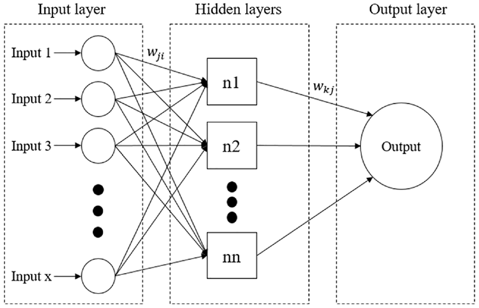
Three-layer neural network (NN) structure.

On the other hand, overfitting problems may occur because of too many hidden nodes, leading to feeble forecasting ability ( 27 ). Although an overfitted model gives a good in-sample fit to the training data, it leads to poor predictive out-of-sample performance. Therefore, both in-sample and out-of-sample behavior examinations will provide information on when and how overfitting occurs. Early stopping as a form of regularization while training a model with an iterative method was implemented to update the model to make it better fit the training data with each iteration ( 37 ). This technique guides as to how many iterations can be run before the model begins to overfit.

Researchers disaccord about the number of hidden layers that are usually selected according to validation checks. Selecting the hidden nodes is consistent with the optimum of hidden layer neurons being determined empirically ( 38 ). In this study, the model’s optimal hyper-parameters are found by the grid-search method, which results in the most precise forecast ( 39 ). Parameters have sometimes been dropped out through this process to minimize over-fitting by avoiding complex co-adaptations to training data and achieving an efficient NN structure.

Weights interconnect neurons as the main parts of each layer. The process of estimating or training the weights of the MLP-NN is usually performed using the back-propagation algorithm discussed in training and testing algorithm of the neural network section. Each neuron calculates its output through its activation function (usually a sigmoid activation function) that can be linear or non-linear.

Training and Testing Algorithm of the Neural Network (NN)

In two successive steps, the NN’s training process is usually accomplished using a back-propagation algorithm, also known as the generalized Delta rule. In the first step, called forward propagation, the sample signals from the training set are inserted into the network inputs and propagated layer by layer until the corresponding outputs are produced. Then, the NN output responses are compared with available desired responses. The training procedure is repeated until a user-supplied stopping criterion such as MSE or coefficient of determination is satisfied.

After introducing the learning samples, modifying the weights/bias, and following a particular learning algorithm, it is checked if the convergence criterion was achieved, and if not, the process is repeated, and all the patterns are again introduced ( 40 ). Therefore, by defining a fixed number of epochs, establishing a performance value to end training and early stop rules convergence of NN is guaranteed.

Choosing an appropriate training algorithm is of great importance. In dynamic NNs, training is performed with the Levenberg-Marquardt back-propagation algorithm (LMBPA), based on optimization to produce the best performance in solving function approximation problems ( 41 ). The sum of the squared differences between the function and the observed data points is minimized during the algorithm ( 42 ). LMBPA benefits from two methods, as it incorporates the steepest descent and Gauss-Newton methods together. When the outputs by NN demonstrate results far from the correct one, the algorithm acts as a steepest descent method: “slow, but guaranteed to converge.”

The network performance is checked after the training phase is stopped. The weights become adjusted with the back-propagation algorithm in the gradient’s negative direction in which the performance function decreases most quickly ( 43 ).

In this paper, the Neural Network Toolbox Version 15b, in MATLAB’s numerical computing environment and its programming language, is used to facilitate the calculation of future marine traffic. The data used for creating NN models are divided into three sets: training, validation, and test. Based on data characters and data size, 70%, 15%, and 15% of data are selected randomly as inputs for training, validation, and testing, respectively. The validation performance is checked in each epoch according to validation errors during the training process. It usually decreases during the initial phase of the training; however, it increases when the network begins to overfit the data. The test phase is used to check whether the trained network can produce desired outputs over a set of data that it has not seen before.

ARIMA Models

The traditional Box-Jenkins ARIMA models as a standard technique used on fitting stationary random series are used in the present paper to model the traffic data ( 44 ). Past values of a time series, in combination with past and present values of a random series, is used to forecast the variables from past and present values with a mathematical model. It should be mentioned that this methodology does not assume any pattern for historical data series to be forecast, whereas, through a three-step iterative approach—model identification, parameter estimation, and diagnostic checking—the best frugal ARIMA model is determined. The ultimate satisfactory model obtained after several iterations can be used to forecast future values ( 45 ). This iterative process for estimating the parameters is conducted to ensure the adequacy of model fit to the data. The model’s ability to produce reliable future data is checked by cross-validation, and the forecasting accuracy is calculated by MSE.

So, the proposed forecasting methodology entails the following steps: (i) Test for stationarity, (ii) Model-identification, (iii) Using penalty functions to choose the best model, (iv) Diagnostic checking, and (v) Forecasting and forecast evaluation.

Test for Stationarity

Stationarity tests are essential, since the stochastic properties like moments (mean, variance, and covariance) of the underlying time series must be time-invariant. Commonly, this process is performed using a correlogram, which is a qualitative and visual aid for defining the trend. Also, the Phillips-Perron (PP) test and the Kwiatkowski-Phillips-Schmidt-Shin (KPSS) test as a unit root test are used to analyze the stationarity of the time series (46, 47).

Model Identification

After checking stationarity, models and parameters should be specified.

Traditional ARIMA Model

An ARIMA (p, q, d) model is generally specified with three parameters to analyze the time series: autoregressive order (p), moving average order (q), and the number of differentials made to be a stationary series (d). If a time series shows periodic behavior after each time interval d, the time series is seasonal in order d. The equation of an ARIMA model (p, d, q) for a time series sequence can be written as:

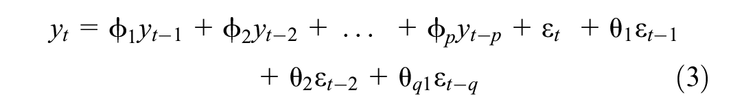
y_{t} = ϕ_{1} y_{t - 1} + ϕ_{2} y_{t - 2} + \dots + ϕ_{p} y_{t - p} + ε_{t} + θ_{1} ε_{t - 1} + θ_{2} ε_{t - 2} + θ_{q 1} ε_{t - q}

(3)

where

$y_{t}$ = the time series,

$y_{t - p}$ = the different lags of time series,

ϕ and θ = the unknown parameters,

p = the order of the AR process,

q = the order of the MA process,

d = the order of differencing, and

ε = the terms that are distributed independently and identically.

In general, four main components affect a time series:

Trend (a general tendency of a time series to increase, decrease, or stagnate over a long time)

Cyclical (medium-term changes in the series, caused by circumstances, which repeat in cycles)

Seasonal (fluctuations within a year during the season) and

Irregular components (random variations in a time series are caused by unpredictable influences that are not regular and do not repeat in a particular pattern)

While four components of a time series are not necessarily independent and can affect one another, a seasonal model is used. The relation between time series components is as below:

Y (t) = T (t) \times S (t) \times C (t) \times I (t)

(4)

where

Y(t) = the observation,

T(t) = the trend at time t,

S(t) = the seasonal variation at time t,

C(t) = the cyclical variation at time t, and

I(t) = the irregular variation at time t ( 45 ).

SARIMA Model

Seasonal or periodic modifications of simple ARIMA models produce SARIMA models. When SARIMA models are fitted to logged data, they can capture seasonal patterns ( 48 ). In SARIMA (p, d, q) (P,D,Q)_s models for a time series sequences, P is the order of the seasonal autoregressive model, Q is the order of the seasonal moving average model, and D is the number of seasonal differences, and s is the periodic term ( 49 ).

Because of the shortcomings of autocorrelogram plots, information criteria or penalty function criteria are widely used to overcome the possible deficiencies. To sum up, the SARIMA models are based on the central premise that the seasonal dependency relationship is the same for all periods. In the case of modeling linear problems, SARIMA models are known for their high precision. However, they require a lot of experience and expertise to forecast appropriately, have difficulty modeling non-linear patterns hidden in the original data, and are sensitive to outliers ( 50 ).

A suitable model order was found using different ARIMA types and orders. In this research, SARIMA models are used to forecast container traffic from 2020 to 2025.

Penalty Functions

The Akaike information criterion (AIC) and the Bayesian information criterion (BIC) are two penalty function statistics that are used for selecting the best forecasting model ( 51 ). AIC estimates and compares each model’s quality with other models and establishes a means for selecting models. AIC combines the error control process and the maximum likelihood principle into one framework to control the forecasting error and have a measure of fit.

Diagnostic Checking

Statistical assessment of chosen SARIMA models by evaluating residuals is essential to prevent probable misspecifications. In diagnostic checks, residuals should resemble a white noise process to have no misspecification. During this process, a diagnostic tool is utilized to plot the model’s residuals against time and real data to diagnose the outliers and autocorrelations.

Performance of the Models

In this research, for testing the performance of NN, the coefficient of determination, or R², is used to determine how well a multiple regression equation fits the sample data. R² is defined as the ratio of explained-to-total variation, taking a value between 0 (no explanation) and 1 (perfect explanation). This measure is as follows:

R^{2} = 1 - \frac{\sum_{i = 1}^{n} {(y_{i} - {\hat{y}}_{i})}^{2}}{\sum_{i = 1}^{n} {({\hat{y}}_{i})}^{2}}

(5)

where

$y_{i}$ = the actual observation,

${\hat{y}}_{i}$ = the value of forecast, and

N = the number of observations.

In both models, forecasting accuracy is measured in relation to MSE over the training, validation, and test sets. This measure of precision is as follows:

MSE = \frac{1}{n} \sum_{i = 1}^{n} {(y_{i} - {\hat{y}}_{i})}^{2}

(6)

where

$y_{i}$ = the actual observation,

${\hat{y}}_{i}$ = the value of forecast, and

N = the number of observations.

This mean-based criterion is a frequently used performance measure ( 52 ). However, using a combination of measures to evaluate the forecast’s accuracy is better than using a single measure. In this research, the performance of the SARIMA models are checked by MSE, MASE, and mean absolute percent error (MAPE):

MASE = mean (\frac{| e_{n} |}{\frac{1}{T - 1} \sum_{t = 2}^{T} | y_{t} - y_{t - 1} |})

(7)

MAPE = \frac{1}{n} \sum_{t = 1}^{n} | \frac{y_{t} - {\hat{y}}_{t}}{y_{t}} | \times 100

(8)

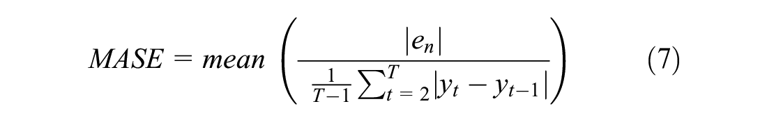
where

${\hat{y}}_{t}$ = the forecast value by the model at time t,

e_n= the forecast error for a given period, and

n = the sample size.

Results

This section applies the NN and SARIMA model to the monthly volume of vessel traffic for container vessels and demonstrates the comparison of SARIMA and NN model forecasting performance. The findings of the forecast achieved from the SARIMA and NN models are shown in the following sections.

Naïve Forecasting Results

According to naïve forecasts, the observed values of the last year are the forecasts for the current year. Although these models are simple, they play a vital role in comparing the forecasting methods. The forecast period was from 2020 to 2025, and error metrics of MSE, MASE, and MAPE were computed for the naïve forecast method (Table 2). Since the number of appeared vessels is few for groups 9 and 10 based on the weak correlation, forecasting may be meaningless. Thus, they are chopped in the calculations.

Table 2.

Mean Square Error (MSE), Mean Absolute Scaled Error (MASE), and Mean Absolute Percentage Error (MAPE) of Naïve Model for all Vessel Groups

Vessel group	MSE	MASE	MAPE
Group (1)	1.7117	1.0473	14.7438
Group (2)	4.5257	1.1416	26.9159
Group (3)	3.6872	1.1427	19.7595
Group (4)	4.9969	1.0063	9.9162
Group (5)	3.8364	0.9754	12.9702
Group (6)	4.3366	0.9861	10.0805
Group (7)	1.7550	0.9672	8.4353
Group (8)	1.5682	0.8903	8.0758

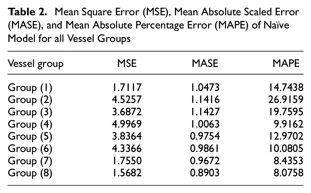
This approach made it possible to evaluate how forecasting accuracy improves with respect to a straightforward, nearly zero-cost approach.

NN Forecasting Results

Forecasting the container traffic is executed in three steps:

Step one: The NN model is applied to annual throughput data from 1999 to 2019 to forecast the future throughput of each DWT category from 2020 to 2025.

For modeling the NN to forecast container traffic, total annual throughput is distributed between 10 DWT-based categories according to the past trend of tonnage distribution of DWT-based categories. Figure 4 depicts the distribution of tonnage between the 10 mentioned categories from 1999 to 2019. The observed trend specifies that the share of more massive vessels increases, and smaller vessels’ share decreases over the years.

Figure 4.

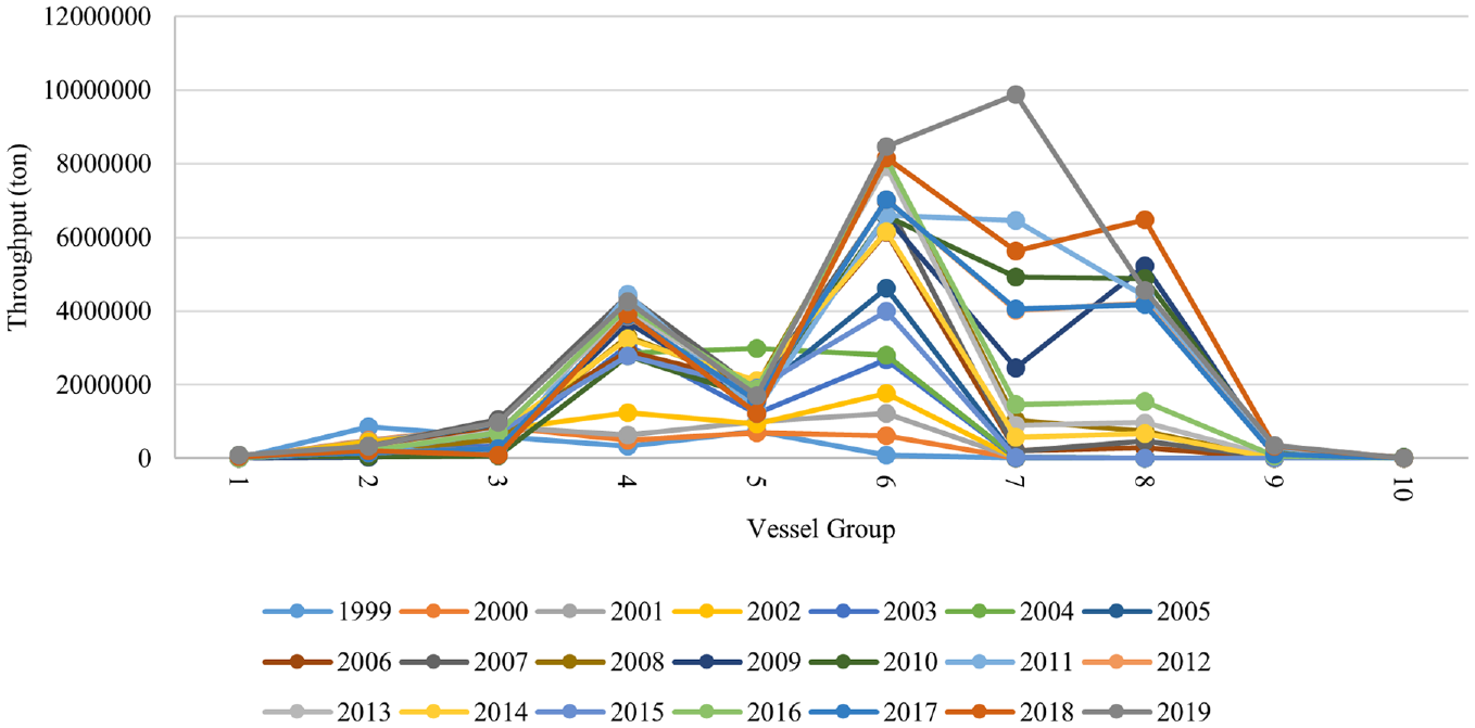
The distribution of throughput between 10 vessel groups from 1999 to 2019.

An MLP-NN with one input layer (annual throughput), one hidden layer, and 10 output layers (tonnage distribution) is used to forecast the future share of each category from each year’s annual throughput. The performance of the NN model with 5, 10, and 15 neurons in the hidden layer to forecast the future distribution of throughput between DWT-based groups is assessed by calculating the correlation coefficient, which is 0.9290, 09378, and 09217 for 5, 10, and 15 hidden neurons, respectively. An NN with 10 neurons in the hidden layer is more prospering than other networks forecasting the future throughput distribution.

Figure 5 illustrates the result of NN with 10 neurons in the hidden layer to forecast the throughput distribution between DWT-based groups and demonstrates the trend which depends on the previous years’ trend.

Figure 5.

The distribution of throughput between 10 deadweight tonnage (DWT)-based groups from 2020 to 2025.

In annual data, the number of observations is less than the requirement for an NN model and several years’ monthly observations are required to model seasonal components appropriately. Therefore, the annual throughput is distributed monthly based on its historical values. Besides, the monthly analysis leads to a more comprehensive analysis of alternative approaches to using judgment on models.

Step 2: The monthly throughput data and the emptiness and fullness of vessels from 1999 to 2019 is used to forecast vessels’ monthly emptiness and fullness from 2020 to 2025.

Because of the correlation between future throughput and the vessels’ size and their emptiness and fullness, input values of emptiness and fullness are forecast with good approximation.

This step compared the benefits of the mean squared error and the correlation coefficient of the test data in multiple constructed networks with a different number of nodes in the hidden layer. It should be mentioned that NNs with 5, 10, and 15 neurons in the hidden layer were used to achieve the best results, and also to present the optimal model for each category depending on the MSE values. Table 3 represents the multi-step performance of the NN model with 5, 10, and 15 neurons in the hidden layer to forecast future vessels’ emptiness and fullness. The NN model is trained with the number of hidden layers more than 15 and less than 5, but the model did not perform correctly.

Table 3.

Optimal Mean Square Error (MSE) in Each Test Case for Forecasting Emptiness and Fullness

Vessel group	5 neurons	10 neurons	15 neurons	Optimal MSE
Group (1)	0.01428	0.00865	0.017621	0.00865
Group (2)	0.00523	0.00615	0.004925	0.00492
Group (3)	0.00148	0.00167	0.001837	0.00148
Group (4)	0.00257	0.00442	0.002604	0.00257
Group (5)	0.00464	0.00401	0.003912	0.00391
Group (6)	0.00285	0.00334	0.004103	0.00285
Group (7)	0.00243	0.00203	0.002982	0.00203
Group (8)	0.00063	0.00150	0.001224	0.00063

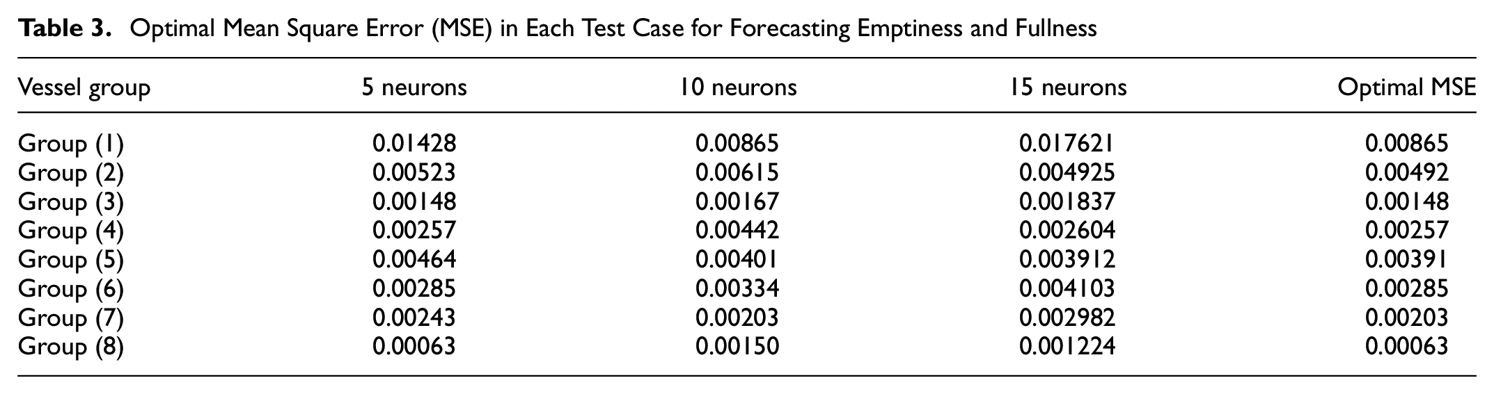
In models with 10 neurons in the hidden layer, the MSE generally reaches its smallest stage. The MSE for each number of neurons is estimated as the average of the MSEs achieved for all forecast groups of vessels (22).

Step 3: Monthly throughput, fullness ratio of vessels, operation type (loading or unloading) and location (in-yard or non-stop) is utilized as inputs in another network to forecast the container traffic from 2020 to 2025.

First, the NN is tested to forecast the container traffic in 2010 and 2011 using the observations from 1999 to 2009. The NN model’s forecasting performance is shown in Figure 6.

Figure 6.

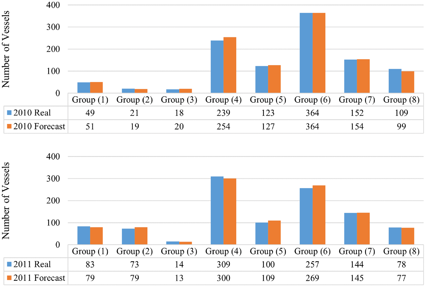
Testing forecasting performance of the neural network (NN) model: (top) year 2010 and (bottom) year 2011.

After testing the NN model, it is used for the primary forecast purpose by using data from 1999 to 2018. A significant trend depicts that, in models with four neurons in the hidden layer, MSE and MASE generally reach their smallest stage. NN performance and regression plots are also analyzed for all cases. The optimal number of epochs shows the iteration at which the validation performance achieved a minimum and stopped training before overfitting. The regression plot reflects a linear regression between the outputs and the respective targets during an NN training phase. Based on Figure A.4, a–h (see Supplemental Material), the outputs match the targets perfectly because the R-value (coefficient of correlation) was > 0.95 in all models and all sets (training, validation, and testing). Table 4 shows the performance of NN with four neurons in the hidden layer.

Table 4.

Mean Square Error (MSE), Mean Absolute Scaled Error (MASE), and Coefficient of Correlation (R²)

Vessel group	MSE	MASE	Coefficient of correlation (R²)
Group (1)	0.07384	0.2502	0.98951
Group (2)	2.77952	0.6466	0.98354
Group (3)	0.85224	0.8207	0.98214
Group (4)	1.31319	0.6398	0.98787
Group (5)	0.29317	0.5372	0.98946
Group (6)	1.14708	0.6791	0.99441
Group (7)	0.01077	0.1019	0.99975
Group (8)	0.03217	0.1468	0.99926

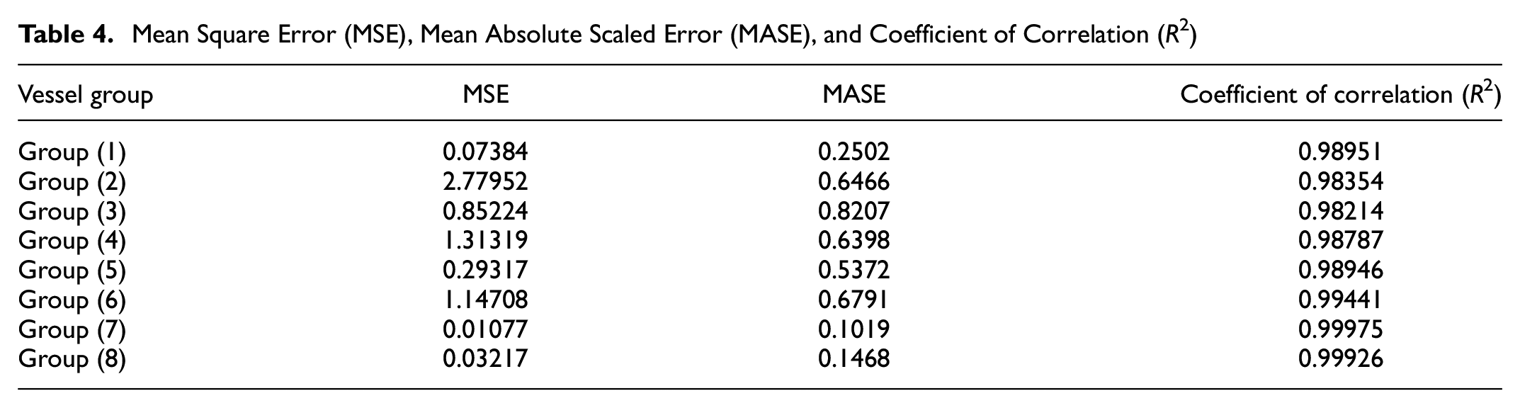
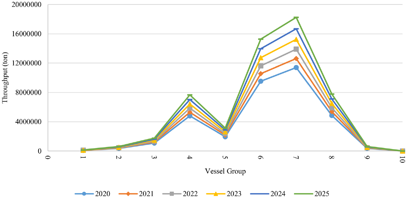
Figure 7 illustrates the results of NN for 6-years-ahead forecast.

Figure 7.

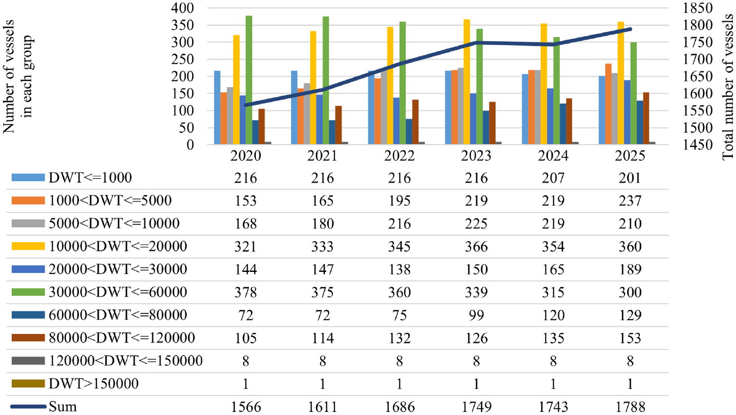
The forecast container traffic from 2020 to 2025 with the neural network (NN) model.

In all steps of work for groups 9 and 10, since the number of vessels which appear is few, the correlation coefficient plot shows a weak correlation so the prediction may be meaningless. So, only some statistical characters are analyzed for it.

Analyzing current conditions and forecasting the future status of the container shipping fleet expresses that the fleet tendency is toward larger vessels. In contrast, the share of small vessels has shown a decreasing trend over recent years. Because of the remarkable growth of large container vessels over the past decade, Panamax vessels continue to be the most common ones, and containers with a capacity higher than 80,000 tones will continue to be the preferred container vessels.

SARIMA Forecasting Results

The database comprises container traffic from 1999 to 2019. Stationary test results reveal that the correlograms of times series have a non-stationary pattern or a unit root with significant lags (Figure 8). Also, PP test and KPSS test reject the null hypothesis and justify the correlogram.

Figure 8.

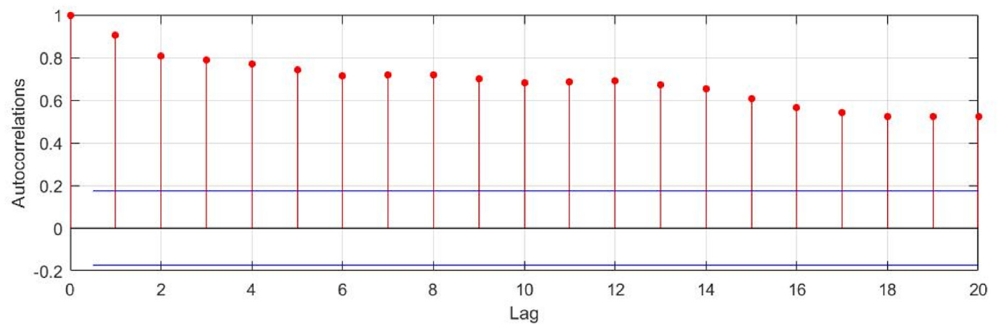
Correlogram representing non-stationarity and seasonality.

The best SARIMA models are selected by trying different models and checking the AIC and BIC values (Table 5). Table A.1 shows the AIC and BIC values of the fitted SARIMA models for all vessel groups.

Table 5.

Akaike Information Criterion (AIC) and Bayesian Information Criterion (BIC) Values of the Fitted Seasonal Autoregressive Integrated Moving Average (SARIMA) Model

SARIMA	AIC	BIC
0, 1, 1	830.34	833.22
0, 1, 2	806.14	809.02
0, 1, 3	830.34	833.22
1, 1, 1	853.19	856.07
1, 1, 2	846.71	849.60
1, 1, 3	856.95	859.83
2, 1, 1	875.48	878.37
2, 1, 2	879.16	882.05
2, 1, 3	884.02	886.91
3, 1, 1	891.13	894.01
3, 1, 2	902.32	905.20
3, 1, 3	902.92	905.80
4, 1, 1	903.67	906.56
4, 1, 2	921.31	924.19
4, 1, 3	917.82	920.71

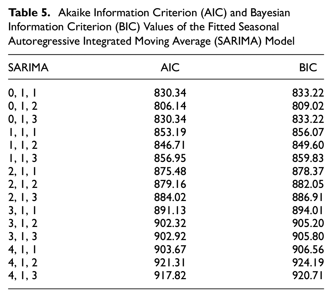
Obviously, among seasonal ARIMA models, ARIMA (0, 1, 2) with the lowest AIC to forecast the future values generates the “best” linear model fitted to the data by the iterative method of model identification, parameter assessment, and diagnostic testing. Table 6 shows the best outputs of SARIMA models for all vessel groups.

Table 6.

Output of Seasonal Autoregressive Integrated Moving Average (SARIMA) Models for All Vessel Groups

		Value	Standard error	t Statistic
Group (1) SARIMA (0, 1, 1)	MA{1}	−0.4182	0.0662	−6.3215
	SMA{12}	−0.7979	0.0616	−12.9522
	Variance	0.8150	0.0696	11.7133
Group (2) SARIMA (0, 1, 2)	MA{2}	−0.2950	0.0688	−4.2876
	SMA{12}	−0.5911	0.0741	−7.9814
	Variance	20.6327	2.2603	9.1284
Group (3) SARIMA (0, 1, 1)	MA{1}	−0.3934	0.0636	−6.1892
	SMA{12}	−0.6863	0.0625	−10.9759
	Variance	14.9554	1.9144	7.8123
Group (4) SARIMA (0,1,1)	MA{1}	−0.6255	0.0615	−10.1771
	SMA{12}	−0.9958	0.0367	−27.0996
	Variance	18.9971	2.1766	8.7280
Group (5) SARIMA (0,1,1)	MA{1}	−0.5874	0.0675	−8.7058
	SMA{12}	−0.6928	0.0796	−8.6997
	Variance	13.1561	1.5505	8.4854
Group (6) SARIMA (0, 1, 1)	MA{1}	−0.6278	0.0654	−9.5984
	SMA{12}	−0.7858	0.0530	−14.8344
	Variance	11.7854	1.2781	9.2211
Group (7) SARIMA (0, 1, 1)	MA{1}	−0.6462	0.0367	−17.5970
	SMA{12}	−0.7734	0.0840	−9.2119
	Variance	0.7119	0.0441	16.1511
Group (8) SARIMA (0, 1, 1)	MA{1}	−0.4847	0.0321	−15.1131
	SMA{12}	−1.0000	0.0976	−10.2474
	Variance	1.4404	0.0821	17.5490

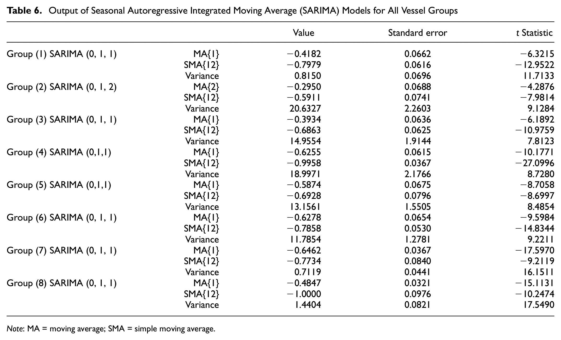
Note: MA = moving average; SMA = simple moving average.

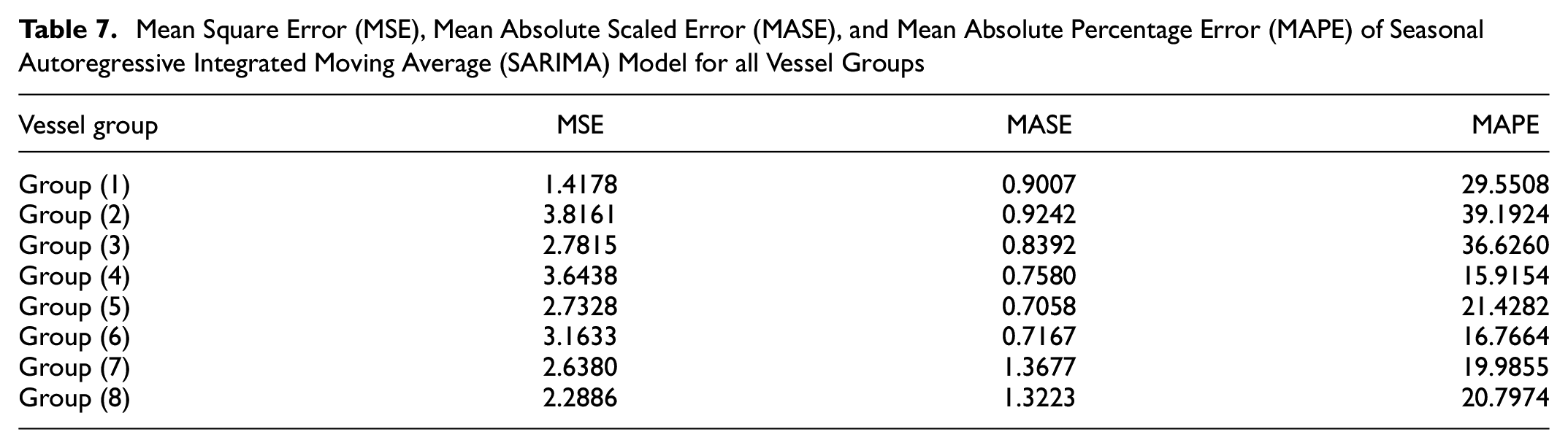
Table 7 shows the performance of the SARIMA model.

Table 7.

Mean Square Error (MSE), Mean Absolute Scaled Error (MASE), and Mean Absolute Percentage Error (MAPE) of Seasonal Autoregressive Integrated Moving Average (SARIMA) Model for all Vessel Groups

Vessel group	MSE	MASE	MAPE
Group (1)	1.4178	0.9007	29.5508
Group (2)	3.8161	0.9242	39.1924
Group (3)	2.7815	0.8392	36.6260
Group (4)	3.6438	0.7580	15.9154
Group (5)	2.7328	0.7058	21.4282
Group (6)	3.1633	0.7167	16.7664
Group (7)	2.6380	1.3677	19.9855
Group (8)	2.2886	1.3223	20.7974

The Ljung-Box Q-test is applied to the residuals of the SARIMA model to test the hypothesis of having no autocorrelation. The Ljung-Box test results are stated in Table 8, which confirms the non-existence of autocorrelation in residuals.

Table 8.

Residual Diagnostic Check for the Selected Seasonal Autoregressive Integrated Moving Average (SARIMA) Model

AC	PAC	Q-stat	p-value
−0.4359	−0.4370	30.2144	3.87E-08
−0.0100	−0.2510	30.2305	2.73E-07
0.0037	−0.1451	30.2328	1.23E-06
0.0969	0.0395	31.7578	2.14E-06
−0.0196	0.0755	31.8205	6.45E-06
−0.1352	−0.1162	34.8281	4.65E-06
0.1562	0.0570	38.8682	2.07E-06
−0.0554	0.0077	39.3798	4.18E-06
0.0059	0.0039	39.3858	9.81E-06
0.0024	0.0302	39.3868	2.17E-05

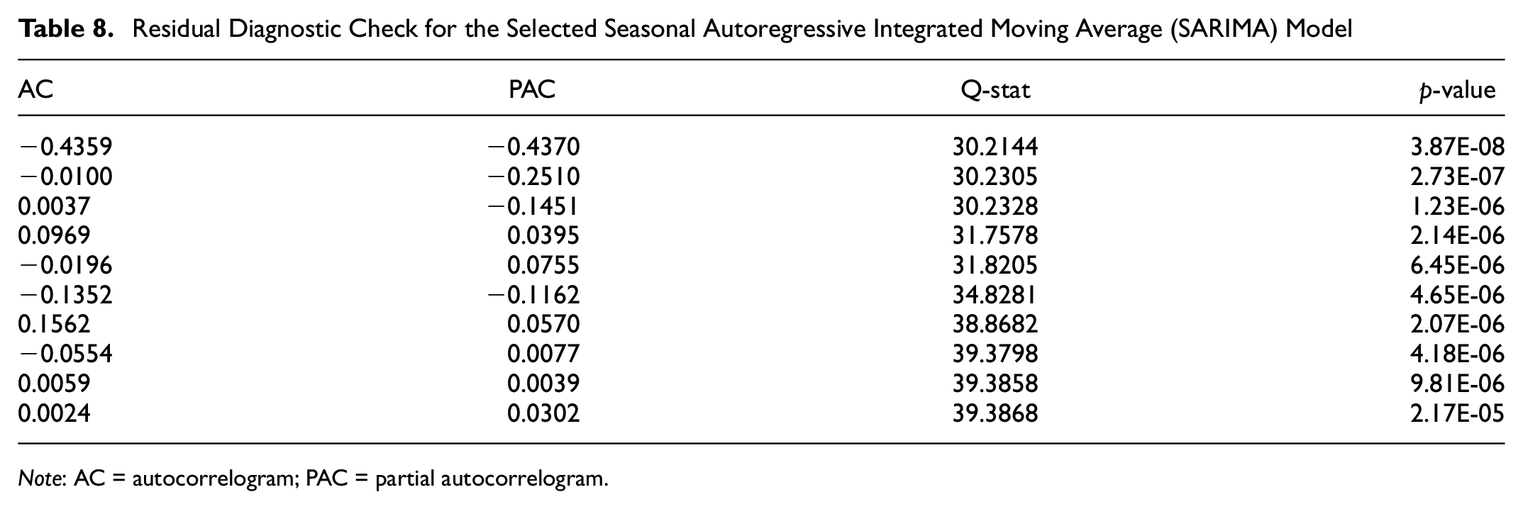
Note: AC = autocorrelogram; PAC = partial autocorrelogram.

Figure 9 depicts that the quantile-quantile (Q-Q) plot of residuals has a normal distribution pattern.

Figure 9.

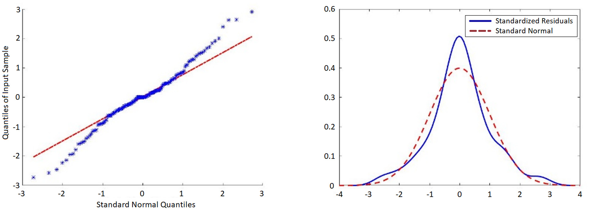
Quantile-Quantile (Q-Q) plot of sample data versus standard normal.

Compared to NN, the outputs match targets in the SARIMA model not very well based on Figure A.5, a–h (Supplemental Material), findings.

Then, SARIMA models are applied to available future throughput volumes to make it possible to forecast the future of container vessels in the target port. Figure 10 illustrates the results of SARIMA for 6-years-ahead forecast.

Figure 10.

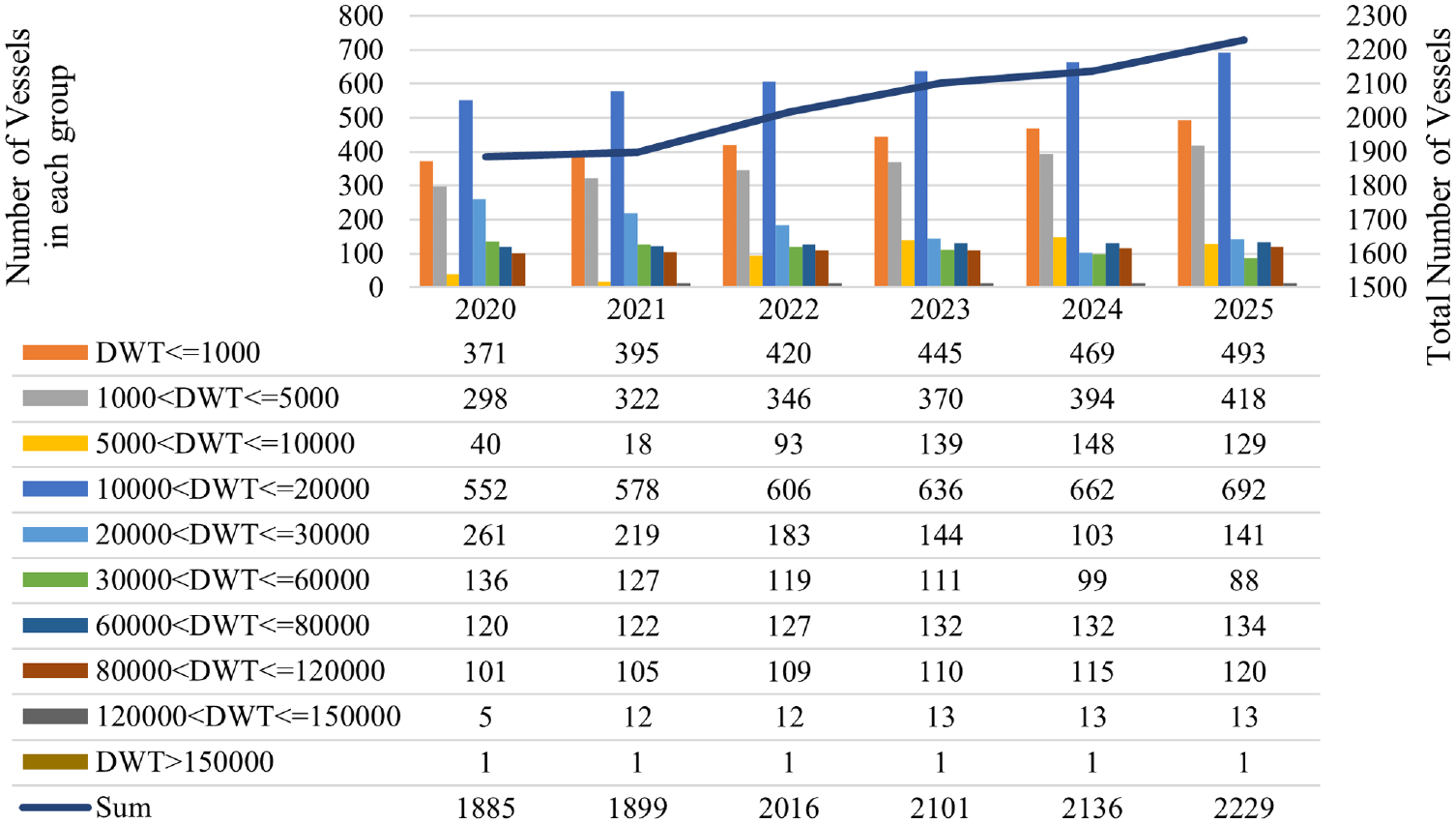
The forecast container traffic from 2020 to 2025 with the seasonal autoregressive integrated moving average (SARIMA) model.

NN and SARIMA Comparison

The final comparison between NN and SARIMA results shows that the NN model results in more accurate outputs than the naïve forecast and SARIMA model. Comparing the MSE and MASE values related to each vessel group (Table 9) verifies the better performance of NN.

Table 9.

Comparison of Mean Square Error (MSE) and Mean Absolute Scaled Error (MASE) between Naïve Model, Neural Network (NN), and Seasonal Autoregressive Integrated Moving Average (SARIMA)

Vessel group	Naïve method		SARIMA model		NN model
	MSE	MASE	MSE	MASE	MSE	MASE
Group (1)	1.7117	1.0473	1.4178	0.9007	0.8584	0.9265
Group (2)	4.5257	1.1416	3.8161	0.9242	2.7795	0.6466
Group (3)	3.6872	1.1427	2.7815	0.8392	0.8522	0.8207
Group (4)	4.9969	1.0063	3.6438	0.7580	1.3131	0.6398
Group (5)	3.8364	0.9754	2.7328	0.7058	0.2931	0.5372
Group (6)	4.3366	0.9861	3.1633	0.7167	1.1470	0.6791
Group (7)	1.7550	0.9672	2.6380	1.3677	0.8053	0.8974
Group (8)	1.5682	0.8903	2.2886	1.3223	0.6800	0.8246

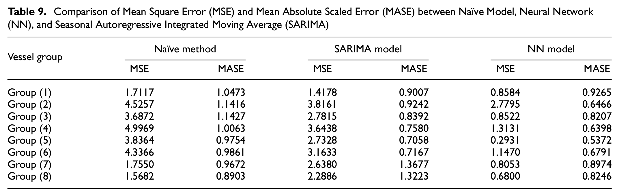
As the NN can obtain different parameters to forecast the trend, the future NN model provided a more accurate forecast than the SARIMA model. The results suggest that the NN model outperformed the other model for vessel traffic forecasting and worked better on the data set to capture the data set pattern.

Discussion and Conclusion

Distinctive characteristics, resources, and liabilities of each port affect different forecasting approaches. Since the best forecasting model and the influential variables are not the same for distinct ports, the discovery of consistent variables and forecasting techniques would reflect truth more precisely. Because of the flexibility and effectiveness in modeling various problems over the past few centuries, both SARIMA and NNs have been frequently used in trend analysis and forecasting. The SARIMA model and the non-linear NNs model were used to capture the different patterns in the data. However, the selection of the best model depends on several factors, including the scope of the forecast, validity and availability of historical data, the degree of accuracy that is desired, the timeline of the forecast, the cost/benefit of the forecast, and the time available for the research. Given the complexity of linear and non-linear data structures, the NN method was conceived as an efficient way to boost forecasting efficiency ( 53 ). Just as this study shows that the appropriate model for forecasting container traffic at Rajaee port is NN, this study also contributes to the knowledge of factors that significantly affect the container traffic, namely monthly throughput, fullness ratio of vessels, operation type (loading or unloading), and location (in-yard or non-stop).

The results revealed that the NN model operated better than the SARIMA model, based on data computing experience and trend. Based on the authors’ experience, the lowest MSE and MASE were achieved in almost all situations for the NN model. The forecasting accuracies are satisfactory, and determination coefficient values exceed 95%. Also, this study demonstrates that the suitable choice of NN inputs and architecture design is critical for the forecasting accuracy of traffic data and model fitting, as appropriate inputs highly affect forecasting behaviors.

Admittedly, this study is restricted to applying NN and SARIMA models to forecast container vessel traffic. It would be interesting to use these models for other vessel types (general cargo, tanker, passenger, etc.). Other linear and non-linear models, such as support-vector machine (SVM), nonlinear autoregressive (NAR), threshold autoregression (TAR), smooth transition autoregressive (STAR), or Holt-Winters models, can be used in future studies to forecast the number of vessels referring to ports. Having said this, the authors believe that the results of this study can assist Rajaee port and other port administrators in dealing with the future container traffic calling ports, as well as coping with the planning and management of yards.

Supplemental Material

sj-docx-1-trr-10.1177_03611981221083311 – Supplemental material for Long-Term Traffic Forecast Using Neural Network and Seasonal Autoregressive Integrated Moving Average: Case of a Container Port

Supplemental material, sj-docx-1-trr-10.1177_03611981221083311 for Long-Term Traffic Forecast Using Neural Network and Seasonal Autoregressive Integrated Moving Average: Case of a Container Port by Negar Sadeghi Gargari, Roozbeh Panahi, Hassan Akbari and Adolf K.Y. Ng in Transportation Research Record

Footnotes

Author Contributions

The authors confirm contribution to the paper as follows: study conception and design: N. Gargari, R. Panahi, H. Akbari; data collection: N. Gargari, R. Panahi; analysis and interpretation of results: N. Gargari, R. Panahi, H. Akbari; draft manuscript preparation: N. Gargari, R. Panahi, H. Akbari, A. Ng. All authors reviewed the results and approved the final version of the manuscript.

Declaration of Conflicting Interests

The author(s) declared no potential conflicts of interest with respect to the research, authorship, and/or publication of this article.

Funding

The author(s) received no financial support for the research, authorship, and/or publication of this article.

ORCID iD

Roozbeh Panahi

Supplemental Material

Supplemental material for this article is available online.

References

UNCTAD. Review of the Maritime Transport. United Nations Conference on Trade and Development, Geneva, Switzerland, 2017.

Memos

C. D.

Port Planning. In Port Engineering ( Tsinker

G. P.

, ed.), John Wiley & Sons, Hoboken, NJ, 2004, pp. 7–64.

Dolman

Containerised and Non-Containerized Trade Through Australian Ports to 2032–33. Bureau of Infrastructure and Regional Economics, Canberra, 2014, pp. 1–142.

Seabrooke

Hui

E. C. M.

Lam

W. H. K.

Wong

G. K. C.

Forecasting Cargo Growth and Regional Role of the Port of Hong Kong. Cities, Vol. 20, No. 1, 2003, pp. 51–64.

Patil

G. R.

Sahu

P. K.

Simultaneous Dynamic Demand Estimation Models for Major Seaports in India. Transportation Letters, Vol. 9, No. 3, 2017, pp. 141–151.

Havenga

J. H.

Eeden

J. V.

Forecasting South African Containers for International Trade: A Commodity-Based Approach. Journal of Transport and Supply Chain Management, Vol. 5, No. 1, 2011. https://doi.org/10.4102/jtscm.v5i1.72.

Nathan Associates Inc. Port Rationalization Study for Trinidad and Tobago. Nathan Associates Incorporated, 2014.

Gökkuş

Ü.

Yildirim

M. S.

Aydin

M. M.

Estimation of Container Traffic at Seaports by Using Several Soft Computing Methods: A Case of Turkish Seaports. Discrete Dynamics in Nature and Society, Vol. 2017, 2017, p. 2984853.

MDS Transmodal Limited. Update of UK Port Demand Forecasts to 2030 & Economic Value of Transhipment Study. Final Report. MDS Transmodal Limited, Chester, 2007.

10.

Holt

C. C.

Forecasting Seasonals and Trends by Exponentially Weighted Moving Averages. International Journal of Forecasting, Vol. 20, No. 1, 2004, pp. 5–10.

11.

Makridakis

Wheelwright

Hyndman

R. J.

Forecasting: Methods and Applications. Wiley, Hoboken, NJ, 1997, pp. 1–632.

12.

Peng

W. Y.

Chu

C. W.

A Comparison of Univariate Methods for Forecasting Container Throughput Volumes. Mathematical and Computer Modelling, Vol. 50, No. 7–8, 2009, pp. 1045–1057. https://doi.org/10.1016/j.mcm.2009.05.027.

13.

Zhong

Angel

Xiumin

Xinglong

Zhixiong

Short-Term Vessel Traffic Flow Forecasting by Using an Improved Kalman Model. Cluster Computing, Vol. 22, No. 10, 2017, pp. 1–10. https://doi.org/10.1007/s10586-017-1491-2.

14.

Ruiz-Aguilar

J. J.

Turias

I. J.

Jiménez-Come.

M. J.

Hybrid Approaches Based on SARIMA and Artificial Neural Networks for Inspection Time Series Forecasting. Transportation Research Part E: Logistics Transportation Review, Vol. 67, 2014, pp. 1–13. https://doi.org/10.1016/j.tre.2014.03.009.

15.

Wang

Shi

Short-Term Traffic Speed Forecasting Hybrid Model Based on Chaos – Wavelet Analysis-Support Vector Machine Theory. Transportation Research Part C: Emerging Technologies, Vol. 27, 2013, pp. 219–232. https://doi.org/10.1016/j.trc.2012.08.004.

16.

Rashed

Meersman

Van

Voorde

Vanelslander

Short-Term Forecast of Container Throughout: An ARIMA-Intervention Model for the Port of Antwerp. Maritime Economics & Logistics, Vol. 19, No. 4, 2017, pp. 749–764. https://doi.org/10.1057/mel.2016.8.

17.

Jugović

Hess

Jugović

T. P.

Traffic Demand Forecasting for Port Services. Promet-Traffic & Transportation, Vol. 23, No. 1, 2011, pp. 59–69.

18.

Bichouh

Port Operations, Planning and Logistics, 1st ed . Informa Law, London, 2009, pp. 2–383.

19.

Farhan

Ong

G. P.

Forecasting Seasonal Container Throughput at International Ports Using SARIMA Models. Maritime Economics & Logistics, Vol. 20, No. 1, 2018, pp. 131–148. https://doi.org/10.1057/mel.2016.13.

20.

Lam

W. H. K.

P. L. P.

Seabrooke

Hui.

E. C. M.

Forecasts and Reliability Analysis of Port Cargo Throughput in Hong Kong. Journal of Urban Planning and Development, Vol. 130, No. 3, 2004, pp. 133–144.

21.

Santos

A. A. P.

Junkes

L. N.

Pires

Jr.

Forecasting Period Charter Rates of VLCC Tankers Through Neural Networks: A Comparison of Alternative Approaches. Maritime Economics & Logistics, Vol. 16, No. 1, 2014, pp. 72–91.

22.

Yang

Mehmed

E. E.

Artificial Neural Networks in Freight Rate Forecasting. Maritime Economics Logistics, Vol. 21, 2019, p. 0123456789. https://doi.org/10.1057/s41278-019-00121-x.

23.

Hassan

L. A. H.

Mahmassani

H. S.

Chen.

Reinforcement Learning Framework for Freight Demand Forecasting to Support Operational Planning Decisions. Transportation Research Part E: Logistics and Transportation Review, Vol. 137, 2020, p. 101926. https://doi.org/10.1016/j.tre.2020.101926.

24.

Zheng

Zhong

Time Series Forecasting Using a Hybrid RBF Neural Network and AR Model Based on Binomial Smoothing. World Academy of Science, Engineering and Technology, Vol. 51, No. 3, 2011, pp. 1464–1468.

25.

Haiyan

Vessel Traffic Flow Forecasting with the Combined Model Based on Support Vector Machine. Proc., 3rd International Conference on Transportation Information and Safety, Wuhan, China, 2015, pp. 695–698.

26.

Container Traffic Forecast Study–Port Metro Vancouver . Vancouver Fraser Port Authority, Vol. 44, 2014. https://www.portvancouver.com/wp-content/uploads/2015/05/2016-Container-Traffic-Forecast-Study-Ocean-Shipping-Consultants.pdf.

27.

Mostafa

M. M.

Forecasting the Suez Canal Traffic: A Neural Network Analysis. Maritime Policy & Management, Vol. 31, No. 2, 2004, pp. 139–156.

28.

Yoo

Jeong

J. S.

Jong

Park

Forecast of Marine Traffic Volume Using Time Series Model. Proc., 2013 International Conference on Fuzzy Theory and its Applications (iFUZZY), Taipei, Taiwan, Vol. 978, 2013, pp. 122–126.

29.

Panahi

Ghasemi Koohi Kheili

Golpira

Future of Container Shipping in Iranian Ports: Traffic and Connectivity Index Forecast. Journal of Advanced Transportation, Vol. 2017, 2017, p. 5847372.

30.

OCDI. Technical Standards and Commentaries for Port and Harbour Facilities in Japan. 2009. http://ocdi.or.jp/tec_st/tec_pdf/tech_00H.pdf.

31.

Radfar

Taherkhani

Panahi

Standardization of the Main Dimensions of Design Container Ships in Ports—A Case Study. World Journal of Engineering and Technology, Vol. 5, No. 4, 2017, pp. 51–61.

32.

Kwak

S. K.

Kim

J. H.

Statistical Data Preparation: Management of Missing Values and Outliers. Korean Journal of Anesthesiology, Vol. 70, No. 4, 2017, pp. 407–411. https://doi.org/10.4097/kjae.2017.70.4.407.

33.

Marine Traffic. MarineTraffic: Global Ship Tracking Intelligence, AIS Marine Traffic. Marine Traffic. 2017. https://www.marinetraffic.com/en/ais/home/centerx:-2.9/centery:59.1/zoom:10%0A.

34.

Dhakal

C. P.

A Naïve Approach for Comparing a Forecast Model. International Journal of Thesis Projects and Dissertations, Vol. 5, No. 1, 2017, pp. 1–3.

35.

Kuźniar

Zając.

Some Methods of Pre-Processing Input Data for Neural Networks. Computer Assisted Methods in Engineering and Science, Vol. 22, No. 2, 2015, pp. 141–151.

36.

Demuth

Beale

Hagan

Neural Network Toolbox, User’s Guide. The Math Works, Inc., Natick, MA, 2004, pp. 1–846.

37.

Montavon

Orr

G. B.

Müller

K.-R.

Neural Networks: Tricks of the Trade. Springer, Berlin, Heidelberg, Vol. 7700, 2012, p. 432. http://scholar.google.com/scholar?hl=en&btnG=Search&q=intitle:Neural+Networks:+Tricks+of+the+Trade#3.

38.

Karsoliya

Approximating Number of Hidden Layer Neurons in Multiple Hidden Layer BPNN Architecture. International Journal of Engineering Trends and Technology, Vol. 3, No. 6, 2012, pp. 714–717.

39.

Bergstra

Bengio

Random Search for Hyper-Parameter Optimization. Journal of Machine Learning Research, Vol. 13, 2012, pp. 281–305.

40.

da Silva

I. N.

Hernane Spatti

Andrade Flauzino

Liboni

L. H. B.

dos Reis Alves

S. F.

Artificial Neural Networks. Springer International Publishing, Cham, 2017, p. 309.

41.

Sapna

Tamilarasi

Kumar

M. P.

Backpropagation Learning Algorithm Based on Levenberg Marquardt Algorithm. Computer Science & Information Technology, Vol. 2, 2012, pp. 393–398.

42.

Gavin

H. P.

The Levenberg-Marquardt Algorithm For Nonlinear Least Squares Curve-Fitting Problems. Department of Civil and Environmental Engineering, Duke University, 2019, pp. 1–19. http://people.duke.edu/~hpgavin/ce281/lm.pdf.

43.

Faruk

D. Ö.

A Hybrid Neural Network and ARIMA Model for Water Quality Time Series Prediction. Engineering Applications of Artificial Intelligence, Vol. 23, No. 4, 2010, pp. 586–594.

44.

Geurts

Box

G. E. P.

Jenkins

G. M.

Time Series Analysis: Forecasting and Control. Journal of Marketing Research, Vol. 14, No. 2, 2006, p. 269.

45.

Adhikari

Agrawal

R. K.

An Introductory Study on Time Series Modeling and Forecasting. arXiv Preprint arXiv:1302.6613, 2013.

46.

Phillips

P. C. B.

Perron.

Testing for a Unit Root in Time Series Regression. Biometrika, Vol. 75, 1998, pp. 335–348.

47.

Kwiatkowski

Phillips

P. C. B.

Schmidt

Shin

Testing the Null Hypothesis of Stationarity Against the Alternative of A Unit Root. How Sure Are We That Economic Time Series Have A Unit Root?

Journal of Econometrics, Vol. 54, No. 1–3, 1992, pp. 159–178.

48.

Mohan

Vedula

Multiplicative Seasonal Arima Model for Longterm Forecasting of Inflows. Water Resources Management, Vol. 9, No. 2, 1995, pp. 115–126.

49.

Chan

H. K.

Zhang

Forecasting the Demand of the Aviation Industry Using Hybrid Time Series SARIMA-SVR Approach. Transportation Research Part E: Logistics and Transportation Review, Vol. 122, 2019, pp. 169–180. https://doi.org/10.1016/j.tre.2018.12.005.

50.

Abhishek

Misra

B. B.

Hybrid Genetic Algorithm and Time Delay Neural Network Model for Forecasting Traffic Flow. Proc., 2nd IEEE International Conference on Engineering and Technology, Coimbatore, India, 2016, pp. 178–183.

51.

Akaike

A New Look at the Statistical Model Identification. IEEE Transactions on Automatic Control, Vol. 19, No. 6, 1974, pp. 716–723.

52.

Wang

Zou

Chaudhry

S. S.

An ARIMA-ANN Hybrid Model for Time Series Forecasting. Systems Research and Behavioral Science, Vol. 30, 2013, pp. 244–259.

53.

Goulielmos

A. M.

Kaselimi.

A Non-Linear Forecasting of Container Traffic: The Case-Study of the Port of Piraeus, 1973-2008. International Journal of Shipping and Transport Logistics, Vol. 3, No. 1, 2011, pp. 72–99.

Supplementary Material

Please find the following supplemental material available below.

For Open Access articles published under a Creative Commons License, all supplemental material carries the same license as the article it is associated with.

For non-Open Access articles published, all supplemental material carries a non-exclusive license, and permission requests for re-use of supplemental material or any part of supplemental material shall be sent directly to the copyright owner as specified in the copyright notice associated with the article.

0.00 MB

0.29 MB