
Abstract
The goal of this study was to analyze the impact of private autonomous vehicles (PAVs), specifically their near-activity location travel patterns, on vehicle miles traveled (VMT). The study proposes an integrated mode choice and simulation-based parking assignment model, along with an iterative solution approach, to analyze the impacts of PAVs on VMT, mode choice, parking lot usage, and other system performance measures. The dynamic simulation-based parking assignment model determines the parking location choice of each traveler as a function of the spatial–temporal demand for parking from the mode choice model, whereas the multinomial logit mode choice model determines mode splits based on the costs and service quality of each travel mode coming, in part, from the parking assignment model. The paper presents a case study to illustrate the power of the modeling framework. The case study varies the percentage of persons with a private vehicle (PV) who own a PAV versus a private conventional vehicle (PCV). The results indicated that PAV owners traveled an extra 0.11 to 1.51 mi compared with PCV owners on average, and the PV mode share was significantly higher for PAV owners. Therefore, as PCVs are converted into PAVs in the future, the results indicate substantial increases in VMT near activity destinations. However, the results also indicated that adjusting parking fees and redistributing parking lot capacities could reduce VMT. The significant increase in VMT from PAVs implies that planners should develop policies to reduce PAV deadheading miles near activity locations, as the automated era comes closer.
Keywords
Over the last 10 years, a large volume of research has focused on modeling and predicting the impacts of autonomous vehicles (AVs) on travel behavior, travel demand, and transportation systems broadly. Although AVs are expected to result in more efficient vehicle operations that improve traffic flow, most studies suggest that AVs will also increase overall vehicle miles traveled (VMT) ( 1 ). Given that AVs are not yet widely available, their overall impact on travel demand and traffic congestion is still uncertain ( 2 ). However, to plan for AVs, including allocating resources for infrastructure investments and setting policies and regulations, it is important to model, understand, and forecast the potential impacts of AVs on transportation systems under a variety of different conditions.
One particular concern about AVs is that they are expected to drastically increase overall VMT and thereby increase congestion, energy consumption, and vehicle emissions. The existing literature identifies a variety of behavioral changes stemming from the introduction of AVs that may increase private vehicle (PV) usage and overall VMT. For example, AVs are expected to decrease the burden or disutility of PV travel as AVs do not require a traveler to drive the vehicle, an onerous and unproductive task, thereby making PV travel less costly and increasing overall travel and travel distances for a variety of trip purposes ( 3 – 5 ). As another example, people without a driver’s license, seniors, and people with medical conditions preventing them from driving are expected to make more trips and increase their vehicle-based travel when AVs enter the market ( 6 ). From a long-term land use perspective, some people may change their home locations and work locations as a result of AVs reducing travel costs to/from major activity locations ( 7 – 9 ). Also, the improved convenience of PVs will attract current transit users to switch trips to PAVs, thereby increasing VMT ( 10 , 11 ).
Additionally, as drivers become riders in PAVs, travel patterns of PAVs are likely to diverge from travel patterns in private conventional (i.e., non-autonomous) vehicles (PCVs). PAV travel patterns are likely to involve dropping off travelers at their exact activity locations and traveling empty (i.e., deadheading) to another location to park during the activity. Although deadheading in PAVs is similar to current taxi and ride-hailing services, in the case of taxis and ride-hailing, the next location is likely to be a traveler pickup spot, whereas in the case of PAVs, the next location is likely a parking spot. Both PAVs and conventional ride-hailing will inevitably generate deadheading miles, that is, vehicles driving without passengers. However, the degree of deadheading in both cases depends on a variety of factors. Recent studies show that deadheading miles from ride-hailing services, unsurprisingly, increase road network congestion ( 12 , 13 ).
This study focused on the near-activity location travel associated with PAVs and their impact on VMT relative to the current world with only PCVs. Figure 1 displays potential travel patterns for PCVs and PAVs for the same person trip from a home location to an activity location. Figure 1 shows that PCV travel typically involves a traveler driving to a parking lot and then walking to the activity location from the parking lot. However, in the case of PAVs, the AV drives the traveler directly to the activity location, negating walking, and then deadheads to a parking location. Notably, because the traveler does not need to walk from the parking location to the activity location, the traveler is more willing to choose parking locations farther away from the activity location (or allow the AV itself to choose more distant parking locations) if they are cheaper.
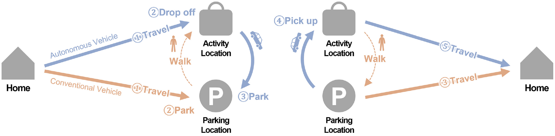
Travel pattern of PCVs and PAVs.Note: PCV = private conventional vehicle; PAV = private autonomous vehicle.
The goal of this study was to develop a modeling framework to analyze the potential impacts of PAVs on near-activity travel patterns and overall VMT. Near-activity travel patterns for PVs denote the travel between activity locations and parking lots by vehicles and people, in cases in which the parking lot is not at the same location as the activity. To model this problem, this paper presents an integrated parking location choice and mode choice model. The parking location choice model considers factors such as parking fee, parking lot capacity and congestion, driving cost per mile, walking distance for PCV travelers, and waiting time for PAVs to pick up travelers for their return home trip. The mode choice model captures the potential shifts between transit, shared vehicles like ridesourcing and taxi, and PVs as a function of the cost and service quality provided by each of these modes. Moreover, by integrating the mode choice and parking choice model, the framework captures the balancing effects of mode shifts toward PAVs (and to a lesser extent PCVs) and parking lot capacity and congestion impacts on the attractiveness of PAVs and PCVs.
The study also presents an iterative solution approach to solve the integrated mode choice and parking location choice problem. The output of the model and solution algorithm includes mode shares, VMT, parking lot occupancy, traveler wait times, traveler walk distances, and traveler in-vehicle travel time (IVTT). By varying the percentage of PAVs and PCVs in various scenarios, the study aimed to analyze the impact of PAVs on overall VMT. The authors believe that integrating mode choice with parking location choice is critical for assessing the impacts of PAVs on near-activity VMT, since PV travel is likely to increase in a future with AVs compared with the current transportation system without AVs.
This paper makes several contributions to the existing literature. First, it introduces an integrated mode choice and parking assignment problem with PAVs, and formulates it as a fixed-point problem, to analyze the impacts of PAVs on near-activity travel patterns and VMT in particular. Previous research has aimed to analyze the impacts of PAVs on travel patterns and VMT, but those studies did not explicitly integrate mode choice and parking assignment. Second, this paper proposes a novel simulation-based parking assignment model to evaluate near-activity travel patterns, VMT, parking lot congestion, traveler walking distance, and other important travel attributes. Third, the paper presents an efficient, iterative solution approach to solve the integrated mode choice and parking assignment problem. Fourth, the paper presents valuable insights into the tradeoffs between VMT, travel time, and travel costs when comparing a system with PCVs versus a system with PAVs. Fifth, the paper provides insights into the role of parking lot prices and the spatial distribution of parking lot capacity can have on VMT.
The remainder of this paper is structured as follows. The next section provides a brief review of the existing literature. The Problem Formulation section presents the mathematical formulation of the integrated mode choice and parking location choice problem. The section that follows this presents an iterative solution approach to solve the integrated model. A case study based on an artificial central business district is outlined in the subsequent section. The computational results from the case study and associated scenario analyses are then presented. The penultimate section discusses the implications of the model results, and the final section presents the conclusions.
Literature Review
Although many studies have analyzed the factors related to AVs that affect travel behavior, relatively few have analyzed the impact of AVs on near-activity location travel and parking. Moreover, most parking studies related to AVs focus on microscopic topics such as optimizing parking lot configurations and how to find a parking location more efficiently ( 14 – 17 ). Conversely, the current study focused on parking and AVs across a transportation network to understand and forecast the potential impacts of AVs on VMT, parking lot usage, and other relevant metrics for transportation planning purposes. This section provides a brief review of studies that analyze the relationship between parking, travel behavior, and transportation system performance for PCVs before reviewing the small set of recent studies that incorporate PAVs alongside the other factors.
The parking location choice problem for PCVs is well established in the literature. Feeney provides a review of studies in the 1970s and early 1980s covering the impact of parking policy measures on travel demand ( 17 ). The behavioral models (mostly logit models) show that factors such as parking fees and time costs (e.g., walking time) affect mode choice and travel behavior ( 18 ). Unlike most of the literature that relies on revealed preference data, Axhausen and Polak employ stated preference data to estimate a parking choice model ( 19 ). Specifically, they create a parking type choice set that includes off-street, surface lot, and multistory parking. Two other studies develop and use agent-based parking choice models within MATSim ( 20 , 21 ). Bischoff and Nagel found that incorporating parking choice in MATSim for Klausenerplatz in Berlin increased total VMT estimates by almost 20% ( 21 ). Habib et al. incorporate parking type choice alongside activity scheduling decisions within an activity-based travel demand model ( 22 ).
More recently, several studies have analyzed changes in parking behavior related to PAVs. Table 1 provides a summary of these studies alongside a summary of the current study. Levin and Boyles adopt the conventional multiclass, four-step, trip-based model to predict PAV travel patterns, assuming some PAVs will drive a traveler to their activity location before deadheading to the same traveler’s origin (home) to avoid parking fees near the high-demand activity center ( 23 ). In a PAV-only scenario, Childress et al. found a 50% discount in parking fees results in a significant increase in VMT ( 24 ). Zhang et al. suggest that PAVs will generate unoccupied VMT because of the reduction of household vehicle ownership and deadheading ( 25 ). Zhang et al. develop an integrated parking choice and route choice model ( 26 ). Harper et al. predict that some PAVs will greedily search for more distant and economical parking spots including unrestricted parking areas rather than downtown parking lots, thereby increasing VMT ( 27 ). On the other hand, Zhao et al. proposed a centrally controlled parking system that collects travelers’ destination information and dispatches the vehicles to the parking lots and found that this can reduce VMT ( 28 ).
Comparison of PAV Studies on Parking Behavior
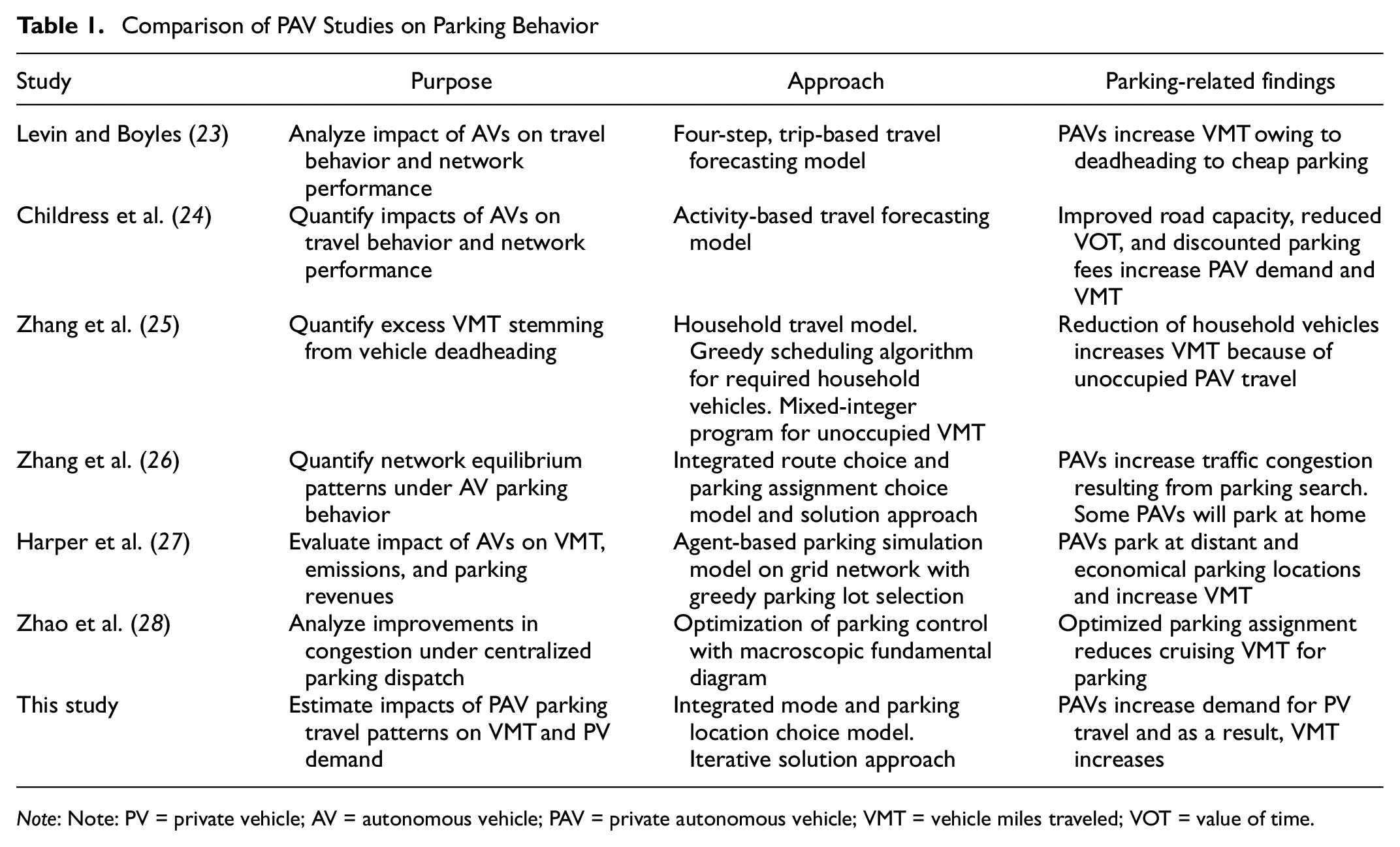
Note: Note: PV = private vehicle; AV = autonomous vehicle; PAV = private autonomous vehicle; VMT = vehicle miles traveled; VOT = value of time.
It is not possible to compare the results of those studies directly since they each make different assumptions and employ different modeling approaches. However, there are several emerging key factors that illustrate the relationship between AVs, travel behavior, and VMT. For example, parking fees and walking time are the most important factors in parking location choice ( 17 – 19 , 24 , 27 ). A vehicle’s cost per mile is a factor as well. For PAVs, waiting time should be included in behavioral models since travelers need to wait for pickup after calling the AV, unless the traveler summons the PAV to arrive at the pickup point first, in which case the PAV may have to wait for the traveler. The model in this study incorporates all of these factors into a utility maximization framework for mode choice and parking location choice.
Problem Formulation
This study presents the integrated mode choice and parking assignment problem, wherein the parking assignment model captures congestion and capacity constraints in parking lots throughout the analysis region. Since the demand for parking is a function of mode choice (i.e., higher PV demand increases parking lot congestion), and mode choice is a function of parking congestion (i.e., congestion in parking lots reduces demand for PVs), this study models the integrated mode choice and parking assignment problem using a fixed-point problem formulation. In general, a fixed point of a function,
Equation 1 displays the general form of the integrated mode choice and parking assignment model in the form of a fixed-point problem. A solution to Equation 1 is a multidimensional array of probabilities,


where
The next section describes the detailed agent-based parking simulation model,
Solution Approach
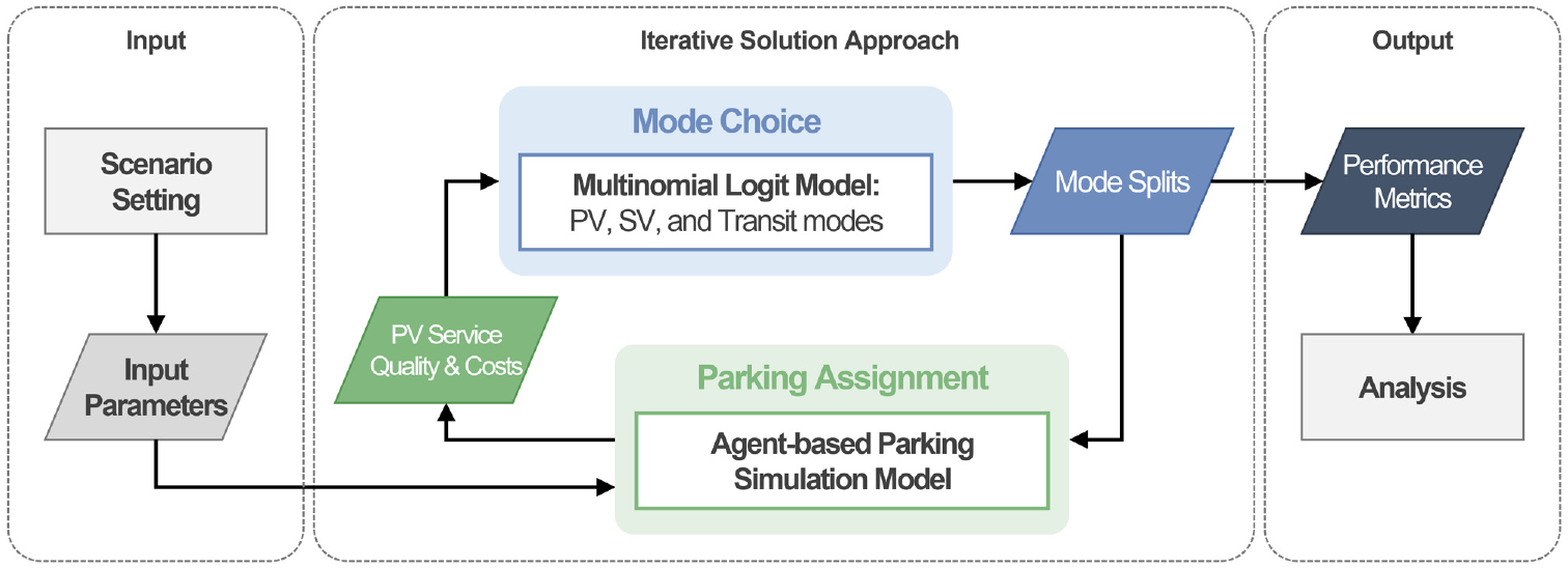
Figure 2 displays the proposed iterative solution approach to solve the integrated mode choice and parking assignment problem. The remainder of the section describes the iterative solution approach along with the model input and output.
Solution approach.
Model Inputs
The left-most box labeled “Input” in Figure 2 includes a scenario setting box that leads into an input parameters box. This study performed sensitivity and scenario analyses based on changes in a variety of model parameters. These parameters and the changes to them are detailed in later sections. The input data and parameters in this study include the available travel modes, mode choice model parameters, fixed modal attributes for nonPV modes, the location, capacity and price of parking lots, parameters for the parking congestion model, the transportation network, and demand data including trip origins and destinations. The following subsections provide details about the available travel models and the mode choice model parameters.
Travel Modes
This study incorporates three types of high-level travel modes, PVs, shared vehicles (SVs), and public transit. PVs include PCVs and PAVs. SVs include shared-use automated vehicles (SAVs,) ride-hailing and ride-sharing services, and taxis. SV travelers wait for a vehicle, travel inside an SV, pay a fare, and receive door-to-door service. Public transit effectively refers to high-capacity buses. Transit riders walk to a bus stop, wait for a bus, pay a fare, travel inside the bus as a rider, and walk to their destination—they may also need to transfer between routes, but this study assumes transfers are not necessary.
Specific scenario details are given in the Case Study section; however, it is important to note that each traveler has access to a single PV—either a PCV or PAV but not both—in this study. Additionally of note, in the scenarios with all PCVs, SVs are conventional vehicles (SCVs); conversely in the scenarios with all PAVs, the SVs are all SAVs.
Mode Choice Model Parameters
Important mode choice model parameters include the disutility of travel time for in-vehicle travel and out-of-vehicle travel (walking and waiting) and the disutility of travel costs. Combining the disutility of travel time and travel costs produces estimates of a user’s value of time (VOT). According to previous studies and reports, VOT varies widely depending on a variety of factors ( 19 , 30 ). Axhausen and Polak found a wide range of walking VOT estimates ranging from $1.35/h to $47.43/h in the mode choice context and $7.67/h to $58.21/h in the parking choice context ( 19 ). Caltrans uses the following VOTs: $13.65/h for automobile and transit in-vehicle VOT and $27.30/h for transit out-of-vehicle VOT in 2016 dollars ( 31 ). Kolarova et al. estimated VOT from the German national household travel survey data, segmented by mode and income class ( 3 ). Based on the middle-income class’s PCV commuting trips ($8.18/h), the other values of in-vehicle VOT were $5.26/h, $8.72/h, and $4.89/h for PAV, SAV, and public transit, respectively. The walking VOT was $12.03/h, whereas the AV and public transit waiting VOT were $9.49/h and $7.45/h, respectively. Zhong et al. provide VOT ranges for PCV, PAV, and SAV in the United States by place of residence: $9.36/h (rural) to $53.71/h (urban) for PCV; $7.71/h to $40.89/h for PAV; and $8.64/h to $46.53/h for SAV ( 5 ). This study mostly used the values in Kolarova et al. ( 3 ).
Moreover, this study used $ 0.50/mi as the cost per vehicle mile of travel, based on the 2020 electric vehicle cost provide by the American Automobile Association ( 32 ).
According to several studies, about 40% of a ride-hailing service travel is deadheading miles ( 13 , 33 ). In other words, when 1 mi of PCV travel from an origin to a destination (except the parking travel distance) is changed to ride-hailing vehicle travel, the travel distance becomes 1.67 mi (67% extra travel). Considering that PAVs do not cruise to find and then pick up another passenger, the PAV’s VMT increase only depends on the empty miles driven from activity location to parking lot.
Iterative Solution Approach
The middle portion of Figure 2 displays an overview of the proposed solution approach that involves iterating between the mode choice model and the dynamic simulation-based parking assignment model. In the iterative process, the output of the parking assignment model is the performance of the transportation system, specifically the costs and service quality attributes associated with PAV and/or PCV travel. Given that the parking model is agent-based, these cost and service quality attributes are available at the agent level and can easily be aggregated over time and space (e.g., travel analysis zones). The costs and service quality attributes for the other modes—transit and SV—were fixed in this study. The costs and service quality modal attributes for PVs from the parking assignment model are the inputs to the mode choice model, alongside the fixed modal attributes for SVs and transit. The outputs of the mode choice model are the modal splits, which are the inputs for the next iteration of the parking assignment model. This iterative process repeats until there is consistency between the mode choice model and the parking assignment model in relation to modal service quality/costs and modal splits.
The following two subsections describe the dynamic simulation-based parking assignment model and the multinomial logit mode choice model, respectively.
Dynamic Simulation-Based Parking Assignment Model
The mode choice model returns modal splits,

where
Each traveler agent in the dynamic simulation-based parking assignment model must choose a parking lot, where

where
The parking assignment model simulates the movements of PAV and PCV travelers and the vehicles themselves as well as the occupancy of parking lots, in a time-driven simulation. Therefore, the simulation captures the current location of travelers, PAVs, and PCVs as well as the current occupancy of all parking lots in the transportation network, every time step, which is denoted
Each traveler has an ordered list of parking lots because it is possible that a parking lot is full when the PV arrives at the parking lot entrance in the simulation, in which case the traveler or the traveler’s PAV needs to travel to the next parking lot on their ordered list. Of note, this study assumes a traveler only becomes aware of a parking lot’s occupancy when they arrive at the parking lot—future studies may assume travelers always have full knowledge of parking lot occupancies. Additionally, since travelers can go from parking lot to parking lot in the simulation, the expected costs for a parking lot
In addition to capturing hard capacity constraints at each parking lot in the transportation network, the parking assignment model also captures in-lot parking search time. This is an important model feature for dense urban areas with limited parking supply, as drivers can spend considerable time inside parking lots finding an open parking spot. In this study, the parking time after entering the parking lot (in-lot parking time) depends on the volume to capacity ratio of the parking lot. For example, this study used a Bureau of Public Roads function to reflect the in-lot parking time, expressed as Equation 7,

where
The parking assignment model also captures network IVTT and network walking time. The simulation model assumes both vehicles and pedestrians travel along the shortest network path. The model does not currently capture congestion in the road network, as the assumption is that parking lot capacity is the limiting constraint on PV mode demand; nor does it capture congestion or capacity at drop-off points (i.e., activity locations).
As noted in Figure 2, the simulation-based parking assignment model returns the service quality and costs for PV modes. It does so by taking the average values for service quality and cost from all traveler agents with origin
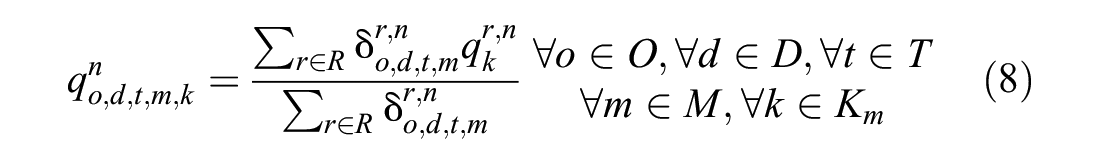
where
The set of experienced service quality or cost metrics,
Multinomial Logit Mode Choice Model
This section describes the mode choice model. The study employed the random utility maximization framework to model mode choice. The utility function for each mode can be written as Equations 9–13,
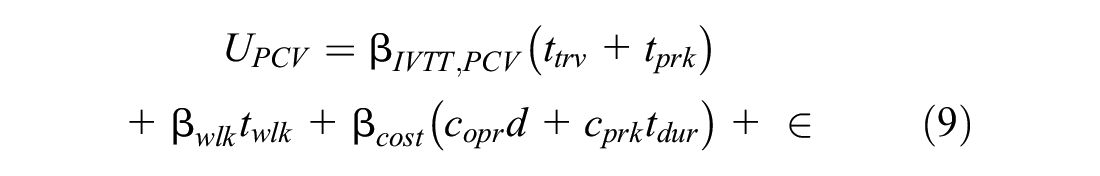
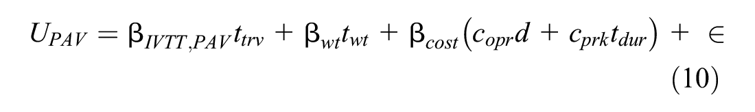


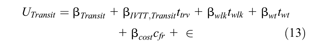
where
Among those variables,
The study also assumes that the error terms,
Model Output
After the iterative solution approach converges to a solution, there are a variety of system-level and agent-level performance metrics that can be output for analysis purposes. The system-level metrics include VMT, empty VMT, final mode splits, parking lot occupancy, and parking lot revenue. The agent-level metrics include travel time, walk time, travel cost, generalized cost, and systematic utility.
Case Study
Network Configuration
This study used a grid network describing an imaginary central business district (CBD). The network, displayed in Figure 3, has 8 external origin nodes (Nodes 1 to 8), 22 activity locations (Nodes 9 to 30), and 10 in-network parking lots (Nodes 31 to 40) with 1 out-of-network parking lot (Node 41) that accommodates unassigned vehicles. The size of a block is 600 × 500 ft and the width of the road is 60 ft. The main road links are unidirectional with a uniform vehicle speed (25 ft/s) and a uniform walking speed (4 ft/s).
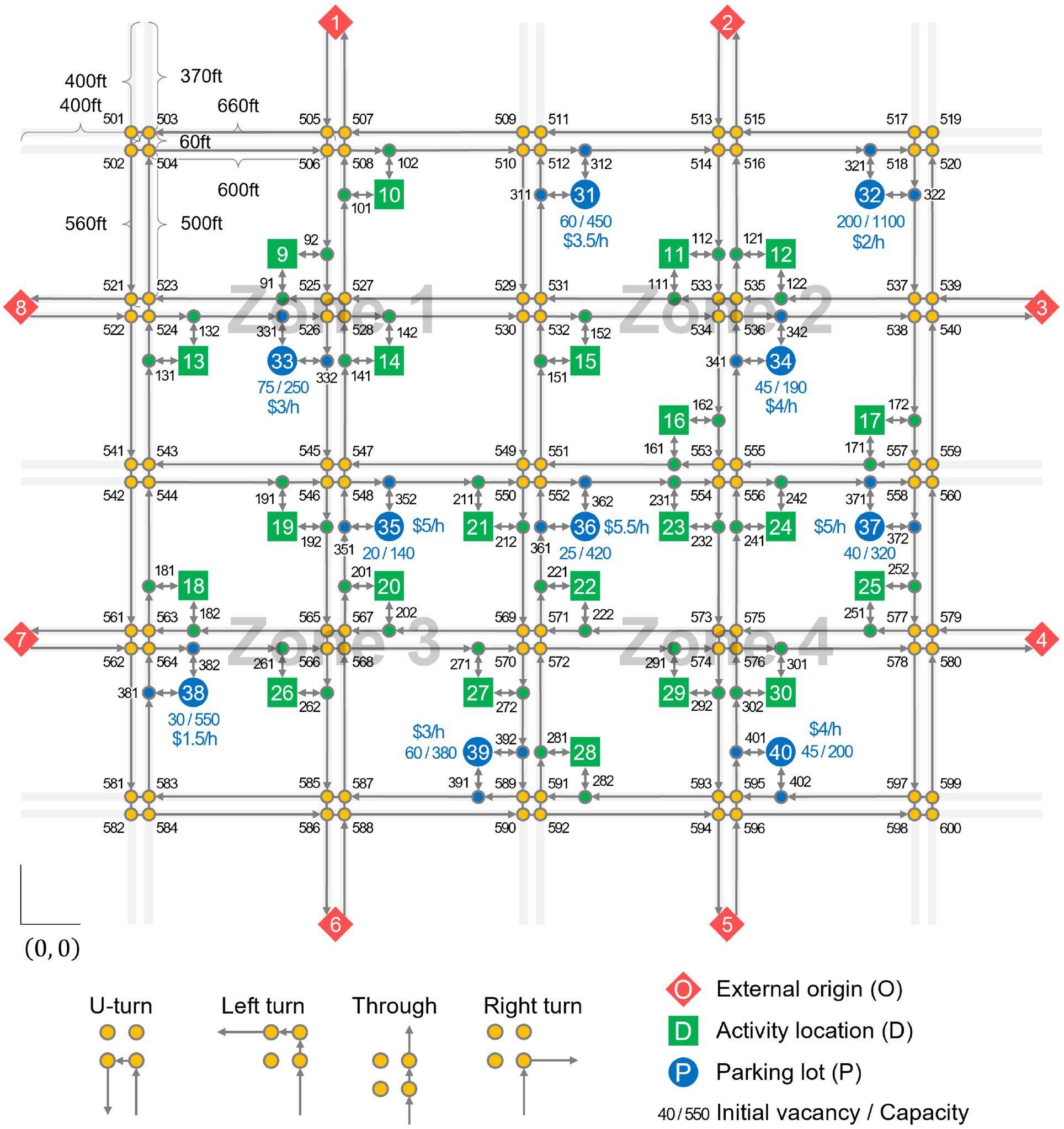
Grid network for parking assignment simulation.
Parking assignment requires a fine spatial resolution, particularly in the CBD. Each intersection is divided into four nodes to reflect intersection delays. Each internal short link in each intersection has additional travel times: 12 s for the through direction and 24 s for a left turn and a U-turn. Each activity location and parking lot has two bidirectional links connected with the main road that take 18 s to traverse and are accessible only from the adjacent direction links (i.e., only right turn is available), and a short detour, such as a U-turn, at the downstream intersection is required for the opposite direction travel. For example, assume a PAV with External Origin 3 and Activity Location 21 parks in Lot 36 in Figure 3, the node sequence of the path would be [3, 539, 537, 122, 535, 533, 531, 529, 530, 549, 550, 212, 21, 211, 550, 552, 362, 36].
Trip Generation and Distribution
Vehicle trips were generated every 6 s (
Parking Lots
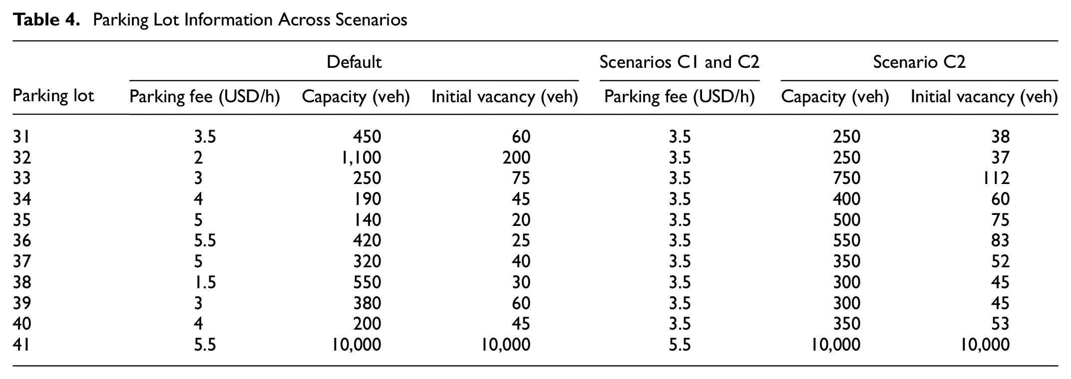
Each parking lot had a fixed parking capacity and a fixed parking fee. The total parking capacity across the 10 parking lots was 4,000 and 15% of parking spots (600) were vacant at the beginning in the base scenario. The Results section includes scenario analyses with respect to changes in parking fees and parking lot capacities. Parking fees ranged from $1.5 to $5.5/h with mean (median) values of $3.65/h ($3.75/h). Parking lot fees were based on lots in major cities in Germany and the United States ( 36 ). When all parking lots were full, vehicles had to go to the out-of-network parking lot (Lot 41), which is 0.5 mi away, costs $5.5/h, and has a capacity of 10,000.
For the in-lot parking space search time function (Equation 7), the study used the following parameter values for all parking lots:
Model Parameters and Values of Time
The model parameters and VOTs used in this study were based on those in Kolarova et al. ( 3 ). Since there is no experience of AV travel yet, the value of AV travel time in most studies relies on SP survey or assumptions. The San Diego Association of Governments multiplies 0.75 from the PCV in-vehicle VOT as a modifier considering the improved convenience ( 37 ), which is the same as Correia et al. ( 38 ). Conversely, Kolarova et al. estimate that in-vehicle VOT in PAVs is 0.64 of in-vehicle VOT in PCVs ( 3 ). According to a review paper by Singleton, several simulation studies assume various VOTs of AVs, and the value ranges from 0% to 100% of PCV VOT ( 39 ). This study applied Kolarova et al.’s survey-based number in the base scenario and adjusted the number in alternative scenarios with different modifiers ( 3 ). Note that Kolarova et al.’s SAV refers to a “driverless taxi” in their survey ( 3 ). The coefficient values used in this study are shown in Table 2.
Model Parameters
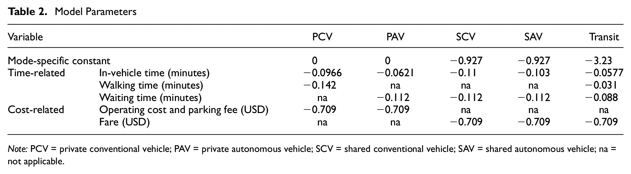
Note: PCV = private conventional vehicle; PAV = private autonomous vehicle; SCV = shared conventional vehicle; SAV = shared autonomous vehicle; na = not applicable.
Travel Costs for Mode Choice
The mode choice model includes out-of-network IVTT since the mode choice is not only based on the travel in the simulated network, but is also affected by the whole travel path. For each traveler, the out-of-network IVTT time for two directions were added to the in-network IVTTs (including the parking lot searching time) determined by the parking assignment model. PV and SAV users’ out-of-network IVTT were set to 20 min per one way, and transit users’ out-of-network IVTT was set to 30 min per one way. Including the in-network IVTT, the total IVTT becomes around the U.S. average (27.6 min for one-way commute) according to recent data ( 40 ). Assuming the average speed is 24 mph, the out-of-network one-way travel distance is 8 mi.
This study assumed 10 min (5 min in each direction) of waiting time for SAV and 20 min (10 + 10) of waiting time and 10 min (5 + 5) of walking time for transit. Transit fare was $5 (thus, $10 for two-way trips). Uber fares consist of a base fare ($2), cost per minute ($ 0.4/min), and cost per mile ($1/mi), which can be changed when the company starts to run AVs ( 41 ). For SAVs, Chen and Kockelman use $ 0.75 to 1.00/mi ( 42 ), Kaddoura et al. assume $ 0.64 to 0.84/mi (€0.35 to 0.46 per kilometer) ( 43 ), and An et al. estimate $ 0.66/min ( 44 ), which is a simplified cost estimation of the current Uber service. Considering those studies, this study used $1.2/mi for SCV fares and $ 0.8/mi for SAV fares.
Scenarios
This study analyzed several scenarios that reflect various possible future conditions at different points in time. Table 3 displays the full set of scenarios. In the base scenario, all PVs were PCVs. Those PCVs were all converted into PAVs in Scenario A. Scenarios B1 and B2 were all PAV scenarios, but they applied different in-vehicle VOTs for PAV, 50% and 90% of PCV in-vehicle VOT, respectively. Scenarios C1 and C2 were also all PAVs but uniformly applied a $3.5/h fee to all parking lots, and Scenario C2 additionally attempted to evenly distribute parking lot capacity across the network. Table 4 displays the parking lot fees, capacity, and initial vacancy across a variety of scenarios.
Scenarios
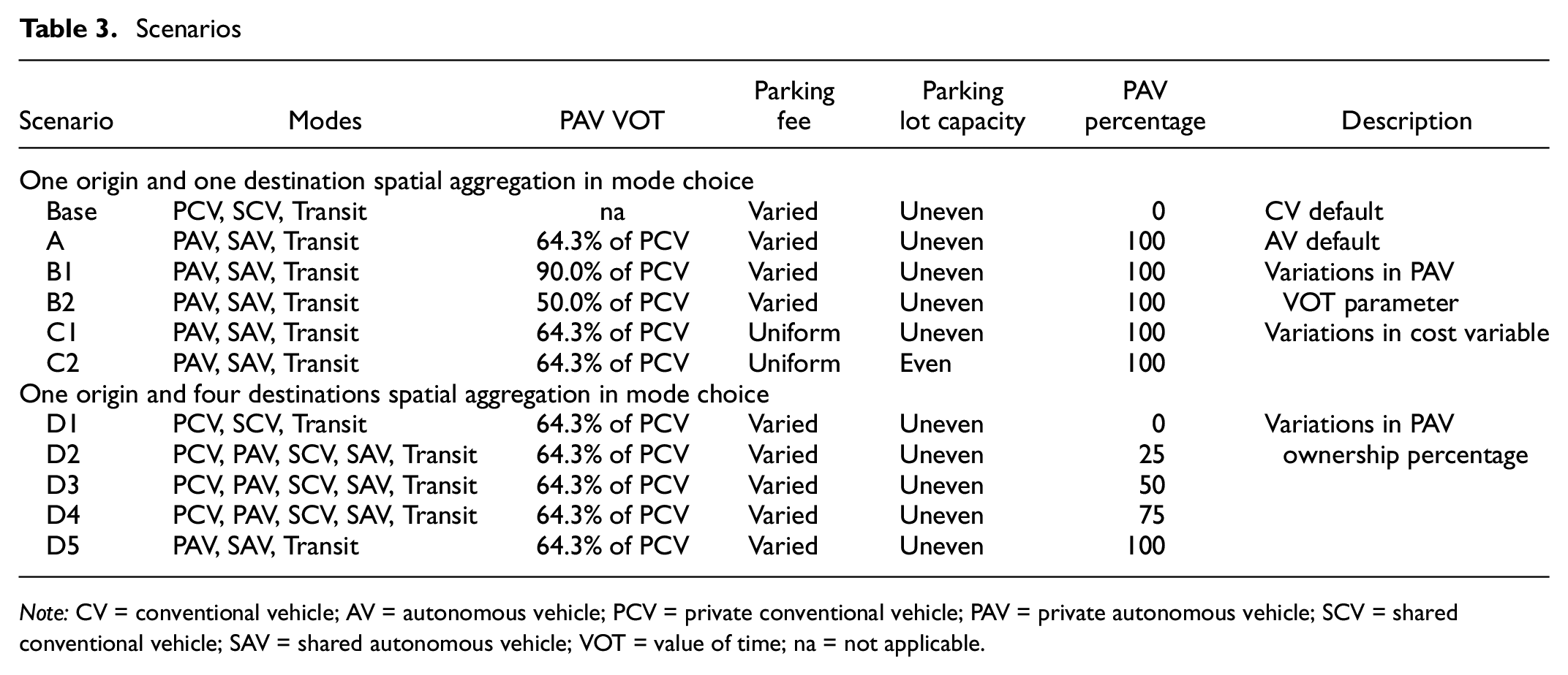
Note: CV = conventional vehicle; AV = autonomous vehicle; PCV = private conventional vehicle; PAV = private autonomous vehicle; SCV = shared conventional vehicle; SAV = shared autonomous vehicle; VOT = value of time; na = not applicable.
Parking Lot Information Across Scenarios
In the base scenario and Scenarios A to C2, the traveler agents were aggregated into a single origin zone and single destination zone for the mode choice model. However, in Scenarios D1 to D5, the traveler agents were aggregated into four destination zones in the mode choice model. Scenarios D1 through D5 varied the proportion of PVs that were PAVs, as opposed to PCVs, between 0 and 1 in increments of 0.25.
Results
No Spatial Disaggregation Scenarios
The Solution Approach section and Figure 2 describe an iterative solution approach to solve the fixed-point integrated mode choice and parking location choice problem,
Figure 4 shows the results of the enumeration approach for the base scenario and Scenarios A through C2. The x-axis displays the input values for the PV mode share,
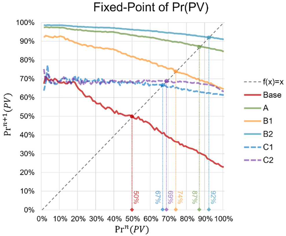
Fixed-point solutions for private vehicle mode choice probability, Pr(PV).Note: Pr(PV) = choice probability of private vehicle.
Using an increment of 1 %, Figure 4 shows that there is a unique solution for the base scenario and Scenarios A through C2. Unsurprisingly, the lines are all downward sloping. Moreover, the relative flatness of Scenarios C1 and C2 likely stems from the parking fees across the network being uniform. The existence and uniqueness of a solution for all scenarios engenders a straightforward analysis of the fixed-point solutions across scenarios.
Mode Share Metrics
Figure 5 shows the mode shares for all modes in each scenario. The mode share for PV was lowest in the base scenario in which the PVs were PCVs, and the mode share was 50%. In Scenario A, in which all PVs were PAVs, PV mode share significantly increased to 87% owing to eliminating walking time, potentially reducing parking fees, and the reduction in IVTT disutility.
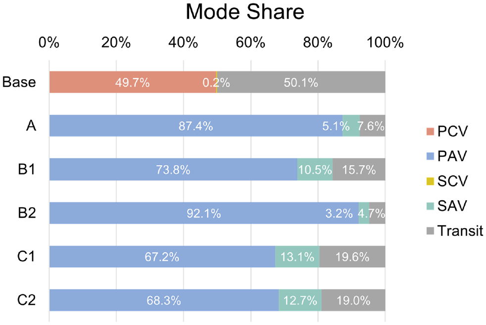
Mode share by scenarios. Note: PCV = private conventional vehicle; PAV = private autonomous vehicle; SCV = shared conventional vehicle; SAV = shared autonomous vehicle.
In Scenario B2, the assumption was that PAV in-vehicle VOT was 50% of PCV in-vehicle VOT, and the PAV mode share increased all the way to 92%. In Scenario B1, when PAV in-vehicle VOT was 90% of PCV in-vehicle VOT, the PAV mode share was 74%. Taken together, Scenarios A, B1, and B2 unsurprisingly indicated that PAV IVTT disutility had a significant impact on mode share.
The properties of parking lots also affected the choice probability. Instead of the varied parking fees that ranged from $1.5 to $5.5/h in the base scenario, all parking fees were set to $3.5/h in Scenarios C1 and C2. In addition, Scenario C2 redistributed the parking lot capacities to be more even in the network. In Scenarios C1 and C2, the PAV mode shares were 67% and 69%, respectively. This represents a notable reduction in mode share compared with Scenario A, in which the larger parking lots had lower fees.
VMT Metrics
In addition to the increase in travel demand (Figure 6a), total PV VMT substantially increased in the PAV scenarios (Figure 6b). Note that we only considered in-network VMT (starting from external origin nodes), and did not include the VMT from the actual origin to external nodes. In-network VMT increased by 15,000 to 22,000 mi in Scenarios A, B1, and B2 compared with the base scenario. Conversely, the increases were reduced when there was no difference in parking fees in Scenarios C1 and C2.
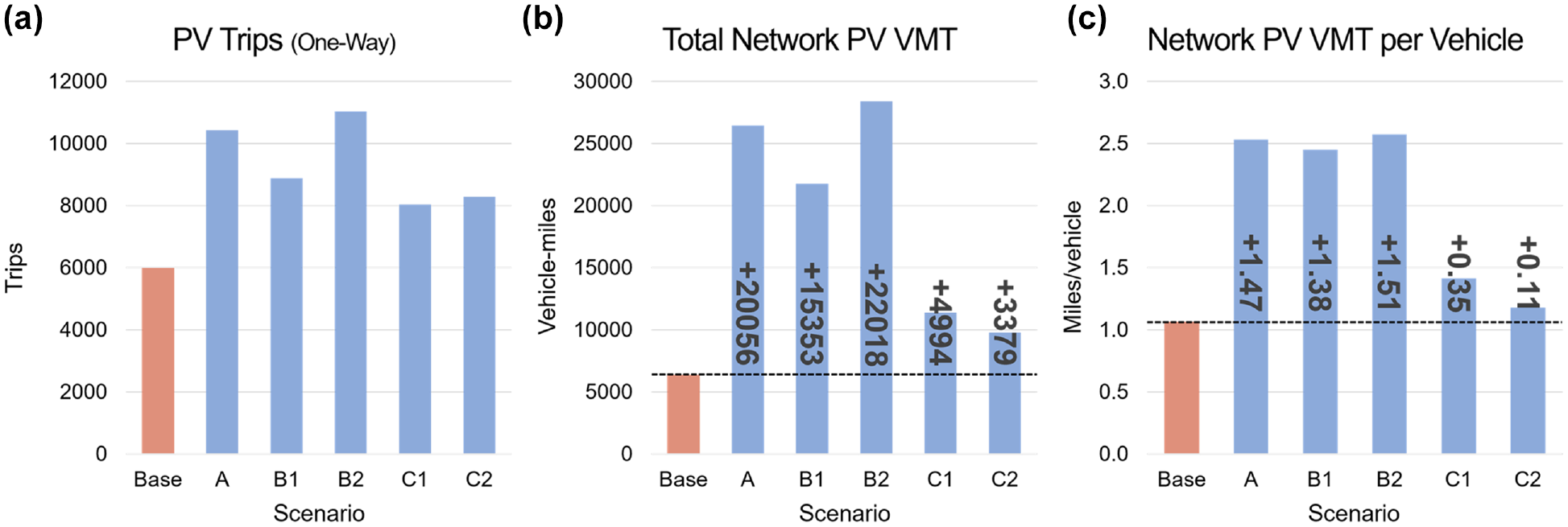
PVs’ VMT in the network: (a) number of PV trips, (b) total PV VMT, and (c) PV VMT per vehicle.Note: PV = private vehicle; VMT = vehicle miles traveled.
As shown in Table 5 and Figure 6c, the average VMT for a PCV was 1.07 mi in the base scenario, and the average VMT for a PAV stretched from 1.18 to 2.57 mi in the other scenarios. The VMT per vehicle increased by 1.38 to 1.51 mi/veh in default parking lot settings compared with the base scenario. In Scenarios C1 and C2, VMT per vehicle increased by only 0.11 to 0.35 mi/veh. This clearly indicated that the spatial distribution of parking prices and parking supply had a significant impact on average VMT per vehicle. Therefore, if policy makers and planners are interested in reducing VMT in a future era with PAVs, parking supply and pricing must be considered alongside other policy measures.
Average PV Traveler Distances and Times.
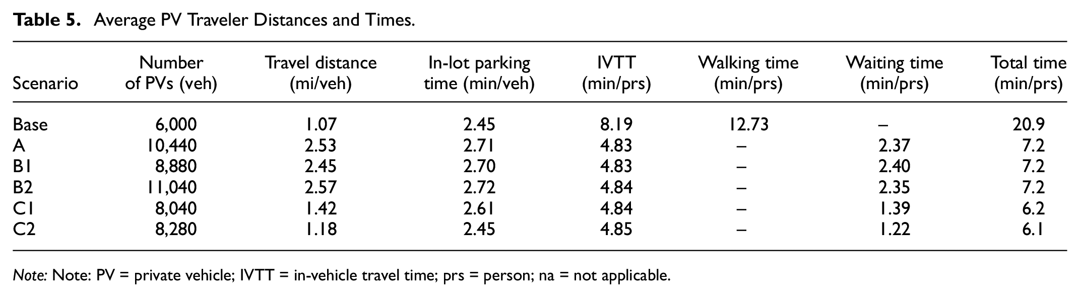
Note: Note: PV = private vehicle; IVTT = in-vehicle travel time; prs = person; na = not applicable.
The increase in in-network VMT from PAVs shown in Figure 6b stemmed from both an increase in PV trips (shown in Figure 6a) and an increase in network VMT per vehicle (shown in Figure 6c). Therefore, VMT in a future with AVs is likely to increase because of travelers switching to PVs and also driving more miles in PAVs than they did or would have done in PCVs. Policy makers interested in decreasing VMT are likely to need a multipronged approach to address these two factors that are expected to increase VMT.
Travel Time and Travel Cost Metrics
Table 5 shows the average travel time components for travelers along several dimensions, along with average total travel time, and average travel distance. Travel distance is the distance in the grid network (counted from the external origin node) and includes the deadheading travel distance. The travel distance in every PAV scenario is longer than the distance in the PCV base scenario.
Since PCV travelers need to travel to parking lots and search for parking, whereas PAV travelers do not, the average IVTT of PCV travelers was 3.3 min longer than that of PAV travelers on average. On the other hand, PAVs spent more time searching for parking than PCVs. The reasons for this were twofold: first, there were more vehicles in the PAV scenarios and, second, PAVs had more homogeneous parking lot preferences—they want cheap parking and are less sensitive to distance from activity location and parking spot search time—making cheaper parking lots more crowded.
The PCV users’ average (one-way) walking time from parking lot to activity location was about 6 min in one direction, and nearly 13 min in total including the activity location to parking lot return walk. Of course, walking time was zero minutes for the PAV scenarios. The average waiting time for PAVs to pick up PAV users was 1.2 to 2.4 min (Table 5). The variation across scenarios comes from the distance between parking lots and activity locations.
The final column sums average traveler IVTT, walking time, and waiting time to determine total travel time. The results showed that the total roundtrip in-network travel time for PCV was significantly higher than total roundtrip in-network travel time for PAV users. Therefore, there were significant time benefits associated with PAVs compared with PCVs.
Table 6 presents an even more holistic comparison of the travel experiences of PV users across scenarios; it includes average monetary costs and monetized travel time components based on the values of IVTT, walking time, and waiting time in the mode choice model. The final column of Table 6 displays the total generalized cost per traveler.
Average Monetized Traveler Costs
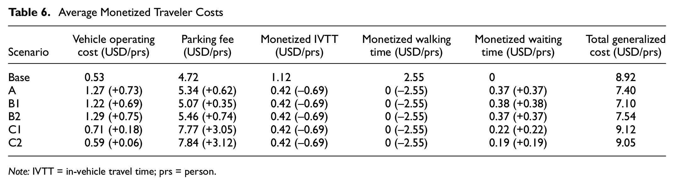
Note: IVTT = in-vehicle travel time; prs = person.
Table 6 shows that the in-network vehicle operating cost was $ 0.06 to 0.75 higher for PAVs than PCVs, depending on the scenario. This result stemmed from the deadheading distance that the PAVs traveled after dropping off travelers at their activity locations.
Scenarios A, B1, and B2 had higher average parking fees for travelers compared with the base scenario. Therefore, despite PAVs being able to travel further to cheap parking lots, the increase in total PV demand in the PAV scenarios forced some travelers to pay for parking at the high-cost parking lots, which more than offset their ability to access cheap parking lots. Since the parking fees were unified in Scenarios C1 and C2, the popular cheaper-than-average parking lots were not cheap anymore. Thus, the average parking fee increased in those scenarios.
The monetized IVTT, monetized walking time, and monetized waiting time columns of Table 6 parallel the IVTT, walking, and waiting time columns in Table 5. IVTT was higher and walking time was significantly higher for PCVs than PAVs, whereas waiting time was higher for PAVs.
The final column of Table 6 is the sum of all the cost and monetized cost components in the preceding columns. Interestingly, although Scenarios A and B1 had the lowest total generalized costs, the base scenario had a lower generalized cost than Scenarios C1 and C2. This latter finding stemmed directly from the high parking cost per person in Scenarios C1 and C2.
Together with the VMT results, Tables 5 and 6 illustrate the tradeoffs between PCVs and PAVs in relation to travel time, travel cost, and VMT. Compared with the base scenario, PAV Scenarios A, B1, and B2 significantly increased VMT, while reducing average traveler in-network time considerably and slightly reducing traveler generalized costs. On the other hand, compared with the base scenario, PAV Scenarios C1 and C2 only slightly increased VMT, while significantly reducing average in-network travel time. However, C1 and C2 had a higher total generalized cost than the baseline scenario because of the higher parking costs that were needed to reduce VMT.
Vehicle Hours Traveled versus Traveler In-Vehicle Travel Time Results
Figure 7 displays both total vehicle hours traveled (VHT) and total traveler IVTT under the various scenarios. Figure 7a displays the total VHT for PVs and traveler IVTT. Even though the number of travelers and VHT increased in the PAV scenarios, there was no significant increase in total traveler IVTT. Understandably, this was because the PAVs were empty during the parking search process. Figure 7b shows that PV VHT per vehicle increased in Scenarios A, B1, and B2 relative to the baseline scenario; conversely, PV VHT per vehicle only increased slightly in Scenario C1, whereas Scenario C2 showed a slight decrease. Figure 7c displays the average IVTT per traveler, with the main result being that IVTT per traveler was lower in the PAV cases than the baseline PCV scenario. The results in Figure 7c partially explained the increase in PV mode share in the PAV scenarios despite the increase in VHT with PAVs.
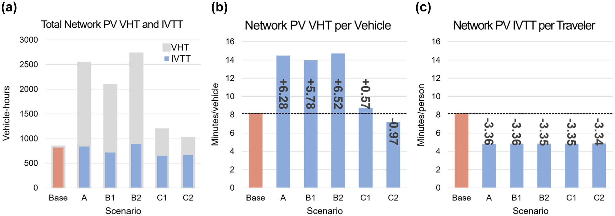
PV VHT and IVTT in the network: (a) total PV VHT and IVTT, (b) PV VHT per vehicle, and (c) PV IVTT per traveler.Note: PV = private vehicle; VHT = vehicle hours traveled; IVTT = in-vehicle travel time.
Impact From Shared Autonomous Vehicles
According to Balding et al. ( 33 ) and Conway et al. ( 46 ), using data from the 2017 National Household Travel Survey ( 45 ), the share of for-hire vehicles (taxi and TNC) is around 0.5% across the country and up to 1.7% in San Francisco and 1.5% in Washington, D.C. Since this study only considered travelers who have their own vehicles, the base scenario (PCV–SCV) showed an even lower mode share for SVs, 0.2%. However, this percentage increased in the PAV–SAV scenarios as the SV’s travel cost per mile decreased significantly.
Naturally, SVs, particularly SAVs, affect total network VMT in addition to PAVs. Assuming 40% deadheading miles for SVs ( 13 , 33 ), SV travel added 0.67 deadhead miles per in-service mile. Figure 8 illustrates the impact of SAVs on VMT. Figure 8a displays the number of SV trips across the scenarios. Interestingly, Scenarios C1 and C2 produced the highest number of SV trips. Figure 8b displays the total SV deadheading VMT, which paralleled the results in Figure 8a. Figure 8c displays the total PV and SV VMT and found that VMT increased substantially (5,000 to 22,000 mi, depending on the scenario) in the AV-based scenarios. However, the impact of SV VMT (green bars in Figure 8c) was relatively small compared with PV VMT (blue bars in Figure 8c) in nearly all scenarios.
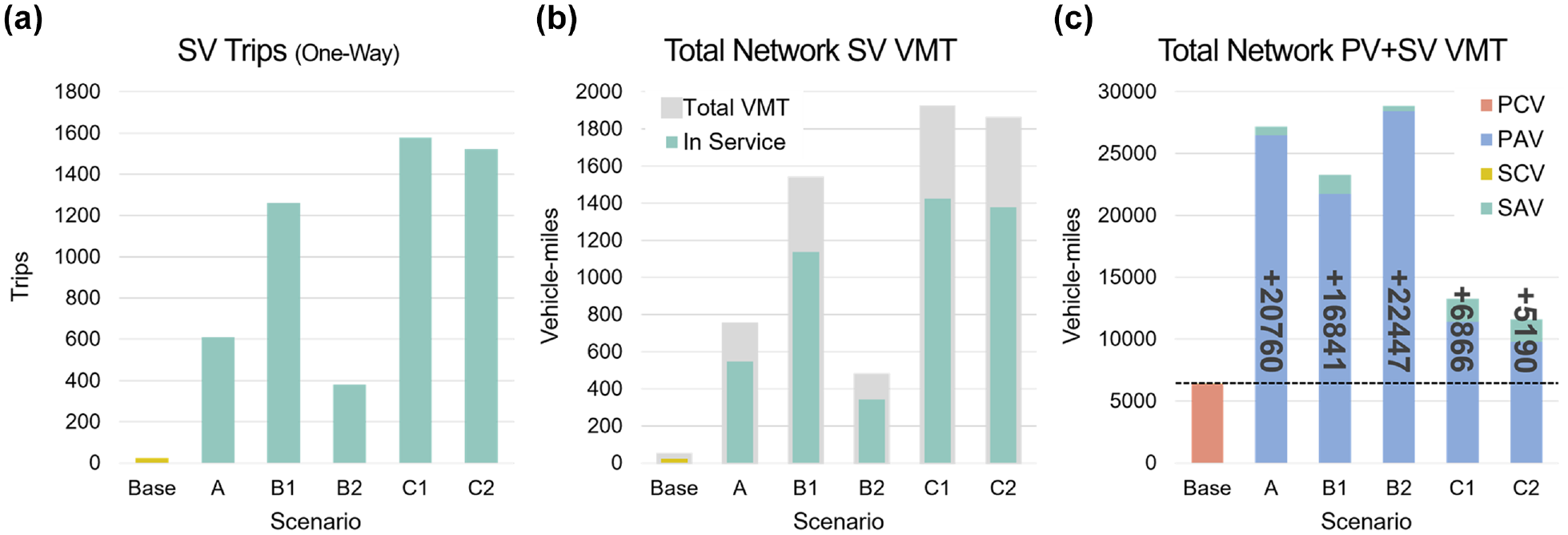
SV VMT in the network: (a) number of SV trips, (b) total SV deadheading VMT, and (c) total PV and SV VMT.Note: PV = private vehicle; SV = shared vehicle; PCV = private conventional vehicle; PAV = private autonomous vehicle; SCV = shared conventional vehicle; SAV = shared autonomous vehicle; VMT = vehicle miles traveled.
Spatial Disaggregation Scenarios
Although the results in the prior subsection were based on an enumeration-based solution approach to the integrated mode choice and parking assignment problem, this section presents the results from using the iterative solution approach proposed in the Solution Approach section. Notably, the iterative solution approach is necessary in this section because the mode choice model aggregates the travelers into four destination zones, rather than just one destination zone like in the prior subsection. This subsection illustrates the ability of the iterative solution approach to identify a solution to the fixed-point problem.
Figure 9 displays the mode choice results under a variety of different scenarios. The parameter
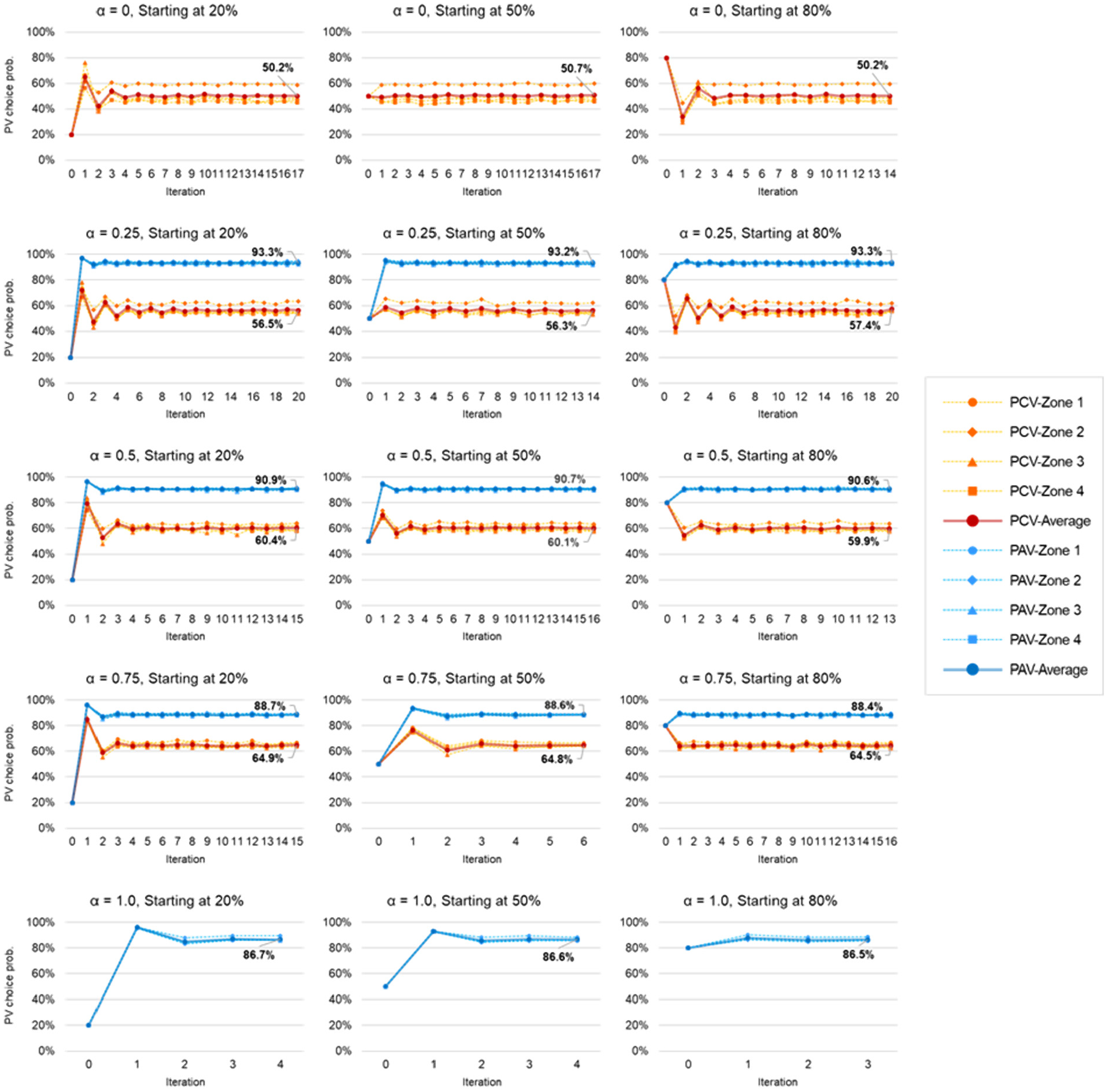
Mode choice convergence plots varying PV mode share starting points by column from 20% to 80%, and PAV ownership proportion by row from 0.0 to 1.0.Note: PV = private vehicle; PCV = private conventional vehicle; PAV = private autonomous vehicle.
The lines in each of the 15 graphs in Figure 9 indicate that the iterative solution approach converged to a fixed-point solution under all cases after less than 20 iterations. Moreover, given that the only thing that changed between the three graphs in each row was the initial starting point of PV mode choice, the 15 graphs indicate that the iterative solution approach found the same fixed point, independent of the starting point of the mode choice probabilities. The analysis below assumes a single fixed-point solution based on the empirical finding in Figure 9 that the algorithm converges to a single fixed-point. However, it is important to note that this paper does not prove that the model system always admits a unique solution.
The results in Figure 9 indicate that PAV owners were much more likely to choose PV than PCV owners, in all scenarios. However, an interesting finding was that as the proportion of travelers who own a PAV,
This logic also explains why the range of modal splits for PCV owners across zones narrowed as
Discussion
Although the case study presented in this paper is based on a fictional CBD, the Results section hopefully illustrates the power of the integrated mode choice and parking location choice model to provide valuable, transferrable, and generalizable insights into VMT, parking occupancy, transportation system performance, and user costs and travel times in a future with PAVs and PCVs. Moreover, the model can be applied to any region if detailed data about the road network, parking lots, and travel demand (or trips) are available. The proposed solution approach, incorporating the simulation-based parking assignment model and the multinomial logit mode choice model, are computationally efficient and would easily scale to large metropolitan areas given data availability.
The proposed model should also be quite useful for policy and planning analysis and decision support. For example, compared with the current PCV-only case, redistributing parking spaces appears able to prevent dramatic increases in VMT while not reducing PV mode share in a future with PAVs. This suggests the spatial distribution of parking supply and parking pricing could significantly affect VMT in a future with PAVs.
Moreover, although not shown explicitly in the Results section, the model can demonstrate, under certain scenarios, that parking pricing alone may struggle to reduce VMT and PV demand. Rather, joint parking pricing and roadway pricing is likely to be necessary in an AV future to reduce VMT and PV demand.
Another implicit finding from this study was that PAVs searching for parking would often look for the cheapest possible lot in the area, particularly when the driving cost per mile was low. Therefore, if all PAVs want to access the same cheap lot(s) in the periphery of the CBD, this/these lot(s) will become full, and the other PAVs will need to search for and drive to the next cheapest lot. This finding has important technology, policy, and modeling implications. From a technology standpoint, providing accurate real-time information to travelers, PAVs, or both about parking lot occupancy could be quite useful. From a policy standpoint, setting parking prices based on disaggregate spatial resolutions in CBDs may not decrease VMT in a world of PAVs. Moreover, there is clearly a value in promoting a reservation system of parking lots and even spaces in parking lots to reduce both parking lot search time and parking space search time, respectively. Finally, from a modeling standpoint, a future extension involves incorporating traveler/PAV knowledge of parking lot occupancy into the modeling framework to analyze the benefits of this information on VMT.
Another future modeling extension involves incorporating roadway congestion into the modeling framework. The results in this paper clearly indicated a significant increase in roadway VMT as a result of the attractive attributes of PAVs as well as the increase in parking search distance for PAVs. However, at some point, if enough vehicles are driving around searching for the cheapest parking lot with available space, the network is going to experience congestion. This increase in congestion would normally have a leveling effect on parking search costs, as human drivers would perceive the time costs of sitting in congestion and probably choose more expensive parking locations and leave the roadway network. However, if the vehicles searching for a cheap parking spot are driverless, they will have much lower costs per minute in congestion and are much less likely to choose nearby parking lots and exit the roadway network. This is a particularly troubling insight for cities in the future. It suggests that congestion pricing in cities may become even more vital to prevent gridlock, and vehicles may need to be charged not just per mile but per minute on the road network to avoid regular gridlock in CBDs.
A related future model extension includes incorporating congestion and capacity constraints at pickup and drop-off spots near activity locations in dense urban areas. With a large percentage of PAVs, SAVs, or both in a dense urban area, large queues are likely to build at pickup and drop-off points associated with activity locations with high demand, such as large office buildings. These queues may even spill over into the roadway network, thereby requiring a response for traffic managers, planners, or regulators.
A final research area includes conducting stated preference surveys to better estimate the model parameters used in this study. Parameters associated with willingness-to-pay, willingness-to-wait, and willingness-to-walk are likely to have a significant impact on model results related to mode share and VMT.
Conclusion
Modeling, understanding, and forecasting the potential impacts of AVs and PAVs on travel behavior, travel demand, and transportation systems under a variety of possible future scenarios is critical for planning for AVs. This study focused on the potential transportation system implications during the transition from PCVs to PAVs for near-activity travel in urban areas. Specifically, given the ability of PAVs to drop off travelers at their activity location and then deadhead to a parking location, under certain assumptions it is conceivable that PAVs will drive great distances to park and/or drive around looking for an open parking space. This process would significantly increase VMT compared with PCVs that drive directly to a parking location close to the traveler’s activity location.
To analyze the impacts of PAVs on near-activity location travel, parking lot usage, overall VMT, and traveler cost and travel time this study proposes an integrated parking assignment and mode choice modeling framework. The proposed mode choice model form is multinomial logit, whereas the parking model is a dynamic simulation-based model of the temporal dynamics of supply and demand for a system of urban parking locations. The study also proposes an iterative solution approach to solve the integrated mode choice and parking assignment problem. In the iterative solution approach, the parking simulation model calculates system performance and costs for travelers based on the demand for each mode—determined either by the mode choice model or the initial modal splits—whereas the mode choice model returns modal splits based on the travel costs from the parking simulation model.
The study applied the integrated model and iterative solution approach to an illustrative CBD network. The model results indicated that PAVs significantly increased VMT compared with PCVs. The reason for this result stemmed from the differential between parking prices and driving fees in the case study. As such, PAVs did not simply look at the stations nearby their traveler’s activity location, instead they considered all parking locations and were highly price sensitive. Consequently, in cases in which a few parking locations are particularly attractive to PAVs, these parking locations may reach capacity, requiring PAVs to detour and search for other parking locations, thereby further increasing VMT in dense urban areas. The Results section also illustrated that PAVs significantly reduced IVTT, eliminated walking time, but required travelers to wait a few minutes to be picked up.
The proposed modeling framework could provide valuable insights to researchers, planners, policy makers, and other city officials in relation to the potential implications of AVs on VMT, parking lot usage, mode share, and other measures of transportation system performance and user costs.
Footnotes
Author Contributions
The authors confirm contribution to the paper as follows: study conception and design: Y. Bahk, M. Hyland; data collection: Y. Bahk, M. Hyland; analysis and interpretation of results: Y. Bahk, M. Hyland, S. An; draft manuscript preparation: Y. Bahk, M. Hyland. All authors reviewed the results and approved the final version of the manuscript.
Declaration of Conflicting Interests
The authors declared no potential conflicts of interest with respect to the research, authorship, and/or publication of this article.
Funding
The authors disclosed receipt of the following financial support for the research, authorship, and/or publication of this article: The first and second authors would like to acknowledge funding support from NSF #2125560 “SCC-IRG Track 1: Revamping Regional Transportation Modeling and Planning to Address Unprecedented Community Needs during the Mobility Revolution.”