Sage Journals: Discover world-class research

Abstract

Unmanned aerial vehicles, or drones, are poised to solve many problems associated with data collection in complex urban environments. Drones are easy to deploy, have a great ability to move and explore the environment, and are relatively cheaper than other data collection methods. This study investigated the use of Cascade Region-based convolutional neural network (R-CNN) networks to enable automatic vehicle counting and tracking in aerial video streams.The presented technique combines feature pyramid networks and a Cascade R-CNN architecture to enable accurate detection and classification of vehicles.The paper discusses the implementation and evaluation of the detection and tracking techniques and highlights their advantages when they are used to collect traffic data.

The substantial growth in population in many urban areas comes at a cost: higher pressure on the transportation infrastructure and increased congestion rates. As a result, transport agencies worldwide are looking for cost-effective and efficient ways to gather realtime information about roads and to respond to unexpected events in a timely manner (1–4). Traditionally, several methods have been used to monitor traffic, including radar sensors, loop detectors, and stationary cameras (5, 6). These methods, however, provide limited information, which is restricted by the ways they are installed or by the road network. They generally lack the ability to provide an inclusive overview of the traffic situation, which is critical for modeling and planning processes. Unmanned aerial vehicles (UAVs), conversely, are more flexible and can cover a wider area by changing their altitude ( 7 ). Drones can facilitate several tasks in management and planning operations including incident, emergency, and parking management; road monitoring and maintenance; and transit operations ( 8 ). They have been used in several studies to understand the kinematic characteristics of moving vehicles (9, 10), to estimate level of service ( 11 ), and estimate O-D matrices ( 12 ).

Using UAVs for traffic monitoring, however, involves several challenges (7, 13). The manual detection of vehicles and traffic flow estimation using images are time consuming, prone to human error, and labor intensive. Automatic detection and classification of moving vehicles would allow the use of UAVs, on a large scale, to monitor traffic, notify operators of accidents, and provide vehicle flow statistics in an efficient manner. Such detection, however, has to be done in a reliable and accurate manner that helps operators respond to events within a reasonable amount of time. A framework was suggested by Khan et al. to enable such automation through five main components: pre-processing, stabilization, geo-registration, vehicle detection and tracking, and trajectory management ( 9 ). In this paper, we focus on vehicle detection and tracking as a fundamental component to enable UAV-based traffic monitoring applications.

Vehicle detection and tracking in aerial images includes many challenges such as variations in viewpoint, scale, illumination, and occlusion. Objects of the same class in aerial images can vary greatly in their size and orientation. Therefore, the detection and identification of objects in such images can vary in nature from typical detection and tracking methods. Early methods, such as in research undertaken by Papageorgiou and Poggio ( 14 ), focus on using complex and domain-specific representations that are optimized for particular classes and shapes. These methods are limited in their ability to deal with the high variability in shapes that are typically associated with aerial images.

Recently, owing to the advances in deep learning ( 15 ) and the availability of large-scale object detection and classification benchmarks (16, 17), the quality of object detection methods has improved significantly. Several high-quality detectors have been proposed such as You Only Look Once (YOLO) ( 18 ), Single Shot MultiBox Detector (SSD) ( 19 ), fully convolutional networks (FCN) ( 20 ), Faster R-CNN ( 21 ), and Mask R-CNN ( 22 ). Several research efforts have used these techniques to allow better estimation of traffic conditions from video feeds. YOLO (23, 24) and FCN ( 25 ) networks have been used to build a vehicle counting and multiobject tracking system from highway traffic surveillance systems. Convolutional neural networks (CNN) have been used in research by Onoro-Rubio and López-Sastre ( 26 ) and Awang and Azmi ( 27 ) to enable automated vehicle counting procedures. Faster R-CNN and Deep SORT (simple online and realtime tracking) ( 28 ) were used in research by Liu et al. ( 29 ) to build a detection–tracking–counting framework.

In this study, we investigated the use of Cascade R-CNN to enable automatic vehicle counting and tracking in aerial images.We present details of the implementation and evaluation of two primary components: (1) a vehicle detection and classification model that scans the aerial image to determine regions of interest (ROIs) and determines the type of objects in these regions; and (2) a multiobject vehicle tracking module that takes the detected objects identified by the first model, assigns a unique identifier (ID) to each object, and identifies these objects in subsequent video frames.

The presented model combines a feature pyramid network (FPN) ( 30 ) and Cascade R-CNN architecture ( 31 ) to deal with detection challenges in aerial images. The FPN produces a multiscale feature representation that allows the detection and classification of vehicles at different spatial resolutions. Cascade R-CNN architecture facilitates the training of a series of detectors that are trained using different intersection over union (IOU) thresholds. It therefore produces more robust region proposals that are less sensitive to occlusion and viewpoint variations. The multiobject vehicle tracking module, which uses a tracking-by-detection technique based on the work presented by Erik Bochinski et al. ( 32 ), is also presented.

The contribution of this paper can be summarized as follows: (1) we investigate the use of FPN as a feature extractor to analyze aerial video feeds and highlight its advantages; (2) we explore the use of Cascade R-CNN to implement automatic counting and tracking-by-detection modules in UAV-based traffic surveillance applications, comparing its advantages to SSDs; and (3) we highlight some of the challenges associated with the training and evaluation of such techniques, including unbalanced datasets, variation in scales, and annotation errors.

Related Work

Recent advances in object detection techniques have enabled a variety of camera-based surveillance systems. The task of object detection is to allow the system to locate different objects within an image or a video frame, which is an essential operation in many applications. In transportation, object detection has been used effectively in several data collection operations such as traffic volume counts, speed estimation, bicycle/pedestrian counts, and vehicle classification. For example, Yang and Qu proposed a detection mechanism based on background modeling ( 33 ). Their technique uses a sparse and low-rank approximation method, which allows the algorithm to be computationally efficient. Background modeling, however, has a major drawback when applied to detect objects in aerial video feeds. The rapidly changing backgrounds makes it difficult to rely on the estimated model in a practical scenario. Other challenges include illumination variation, shadow areas, and scale variations. A similar approach, suggested by M. A. Abdelwahab, uses a narrow region, typically a line, for detecting vehicles when they pass through it ( 34 ). Although this approach is more efficient, it is not robust in the face of changes in drone movements, including changes in altitude and viewpoint variation.

More recently, research efforts have focused on using deep learning approaches to enable more robust object detection mechanisms. Deep CNNs ( 35 ) can produce high-level image representations that can be effectively used to detect objects in a stable and precise manner. Deep learning detection methods can be generally classified into two groups: one-stage detectors such as YOLO ( 18 ) and SSD ( 19 ), and two-stage detectors such as SPP-Net ( 36 ) and Faster R-CNN ( 21 ). Two-stage detectors, as the name indicates, use two networks to propose objects’ regions and then classify objects within these regions. Single-stage detectors produce the regions and classifications using only one network. Generally, two-stage detectors produce more accurate localization results and can detect objects at different scales, at the expense of computational efficiency. Deep learning approaches have been used in several traffic surveillance applications to detect pedestrians ( 37 ), to count vehicles ( 23 ), and in cyclist detection ( 38 ). In this study, we focused on using these approaches to improve vehicle detection and tracking in aerial images.

Another essential task in the analysis of aerial video feeds is multiple object tracking (MOT). MOT algorithms allow the collection of critical information that describes the characteristics of traffic flow and driving behavior. A common technique that is used in several tracking applications is the Kalman filter ( 39 ), which offers a computationally efficient algorithm that provides relatively accurate estimations across a range of tracking scenarios. The Kalman filter has therefore been used in several proposed tracking schemes (33, 40, 41). Recent approaches have focused on extending the capability of the Kalman filter by using features extracted from deep learning networks. A notable example is the SORT algorithm ( 42 ), which uses high-level features extracted by CNN-based networks to conduct robust frame-to-frame associations. In this paper, we focus on assessing the performance of tracking vehicles when the presented detection method is used.

Methodology

The following subsections discuss the components of the system in more detail.

Vehicle Detection and Classification

To illustrate the vehicle detection and classification module, we start by discussing Faster R-CNN architecture, as a foundational architecture. We then discuss the detection model.

Faster R-CNN Architecture

Faster R-CNN architecture ( 21 ), has two main stages, as shown in Figure 1. The first stage, sometimes called the region proposal stage, receives image features and uses them to produce ROIs to identify where the objects are located. Image features are typically extracted via a pretrained deep network such as ResNet ( 15 ). ROIs are generated using a set of anchor boxes that provides a predefined set of reference bounding boxes of different sizes and ratios. Each ROI is associated with an abjectness score, which indicates whether the region contains an object (positive example) or a background (negative example).

Figure 1.

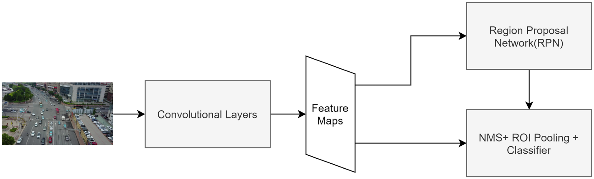
The main components of the Faster region-based convolutional neural network ( 21 ). The abbreviation NMS stands for non-maximum suppression and ROI stands for region of interest.

In the second stage, the classification stage, ROIs, produced by the region proposal network (RPN), are fed to a nonmaximum suppression (NMS) module, which filters out overlapping (and hopefully duplicated) ROIs that have a certain IOU threshold. ROIs’ boundaries are used to crop the part of the convolutional feature maps that corresponds to the proposed region. Cropped parts are scaled using ROI pooling layers and fed to the classifier, which produces the final labels. The classifier produces labels for the regions whose IOUs with ground truth bounding boxes exceed a certain threshold (for positive examples).

The Detection Model

The detection model extends the basic Faster R-CNN base model by using two main components: (1) an FPN, which produces a high-quality and semantically rich feature pyramid, and (2) the Cascade R-CNN architecture, which improves detection performance by training several detectors that use different IOU thresholds. The following subsection discusses the operation of these extensions in more detail.

FPN

The FPN ( 30 ) leverages an appealing property of convolutional networks—the pyramidal feature hierarchy of the output produced by its successive layers. In convolutional networks, because of the subsampling process, layers near the input produce an output that has high spatial resolution but low-level semantics (typically not sufficient to identify objects). Layers near the output, conversely, produce outputs with high-level semantics but low spatial resolution. The FPN uses feature maps from the different layers to construct a pyramid that has high-level semantics at all levels. In our implementation, we used ResNet-101-FPN architecture, which uses a pretrained ResNet as a basis for constructing the pyramid representation.

The operation of the FPN is illustrated in Figure 2. The bottom-up path represents the layers produced by a typical convolutional network such as ResNet ( 15 ). An image is fed to the network as an input, and a feed-forward operation produces different feature maps at different spatial resolutions via a down-sampling process. Whereas top feature maps (layers far from the input) have more semantics (that is, more abstract information about the image), bottom maps have a higher resolution and weaker semantics (more detail but a poorer understanding of the image). FPN extends a typical CNN using the top-down pathway shown in the right-hand side of Figure 2. The network reconstructs bottom layers from top layers using an up-sampling process and lateral connections to the corresponding layers from the bottom-up path. Such reconstructions result in feature maps that have a higher resolution and stronger semantics than the typical CNN layer. Therefore, FPN produces a feature pyramid containing different scale levels in which each scale contains high-level semantics about objects (while maintaining relatively high spatial resolution). This feature pyramid is then fed to the RPN to produce the region proposals and objectness scores mentioned earlier.

Figure 2.

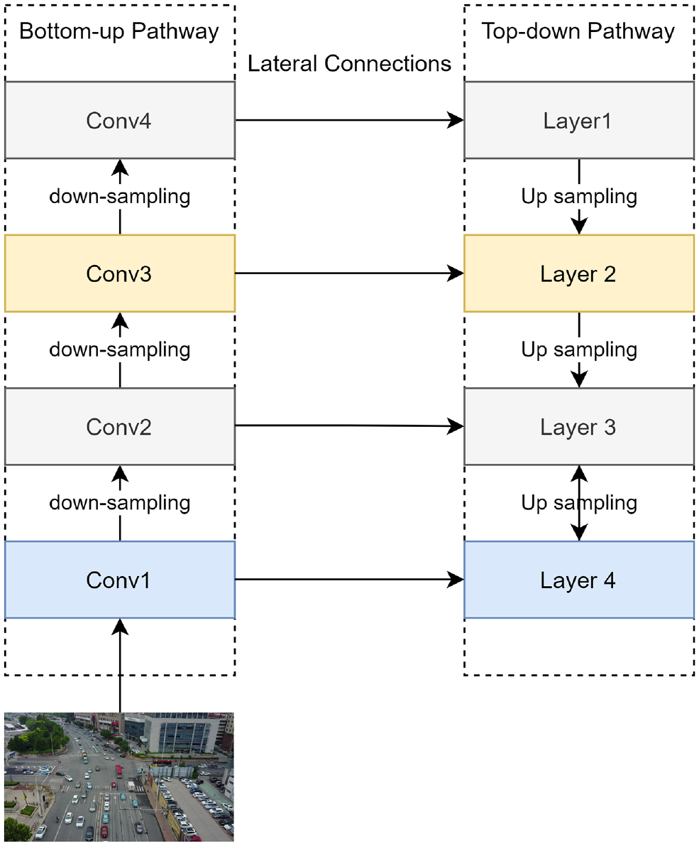
The operation of a feature pyramid network ( 30 ).

Cascade R-CNN

As mentioned previously, object recognition uses an IOU threshold to discriminate positive and negative examples. The choice of this threshold has an impact on the overall performance of the detector. Whereas small threshold values result in noisy bounding boxes, relatively large values may result in poor training performance as the model rejects close positive examples. Because of the high variability in aerial images (viewpoint variations, scale variations, etc.), it is difficult to make an accurate hypothesis about the value of an IOU threshold.

The Cascade R-CNN architecture ( 31 ) is a multistage extension that trains successive detectors with different IOU thresholds. The bounding boxes produced by one R-CNN stage act as an input to train the next stage, as shown in Figure 3. By using multiple specialized regressors, Cascade R-CNN produces high-quality detection by removing noisy detected bounding boxes while keeping useful, close, positive examples.

Figure 3.

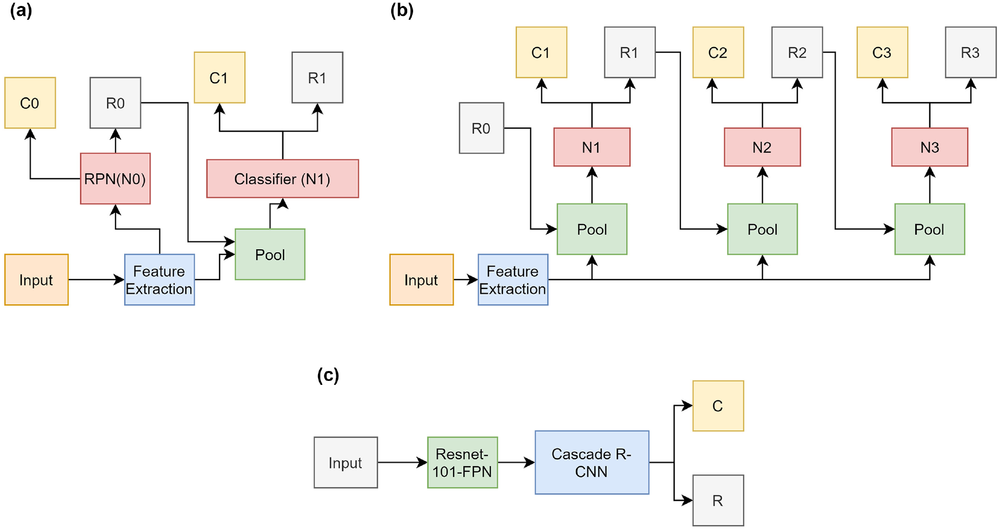
(a) Faster R-CNN, (b) Cascade R-CNN, and (c) Cascade R-CNN + FPN. “R” is proposed regions, “C” is the classification, and “N” is the classifier network. ( 31 ).

Similar to reseach undertaken by Cai and Vasconcelos ( 31 ), the loss function used in the model training is defined as

L (x^{t}, g) = L_{cls} (h_{t} (x^{t}), y^{t}) + λ [y^{t} \geq 1] L_{loc} (f_{t} (x^{t}, b^{t}), g)

(1)

where

$t$ = stage number,

$h_{t}$ = classifier model at stage t,

$f_{t}$ = regressor at stage t optimized for IOU threshold $u^{t}$ , $u^{t}$ > $u^{t - 1}$

where $x^{t}$ is the image patch at stage t; $b^{t}$ is the bounding box at stage t calculated from the previous stage $b^{t} = f_{t - 1} (x^{t - 1}, b^{t - 1})$ ; g is the ground truth object for $x^{t}$ ; $y^{t}$ is equal zero if the $IOU (x^{t}, g)$ < $u^{t}$ , otherwise it is equal to the value of the class number (a value greater than 1) for the ground truth object; and $λ$ is a hyperparameter that is used to control the weight of the localization loss component (this was chosen to be 1 in our implementation, that is, equal weight of the classification and localization components).

Since the data were highly unbalanced, as we will discuss in the upcoming Dataset section, we used a weighted version of the classification loss function, $L_{cls}$ . The weight of each class (c) was calculated such that, c = (size of the classs of the smallest number of objects/size of class c). In addition, the weight of the background class was set to be equal to the weight of the most dominant class (the class of cars in our case).

Multiobject Vehicle Tracking Module

Tracking is performed simply by measuring the IOU between detected objects in two subsequent frames. If a greedy IOU tracking approach is used, the two objects with the highest IOU are assigned the same tracking ID. The basic concept of IOU tracking is illustrated in Figure 4.

Figure 4.

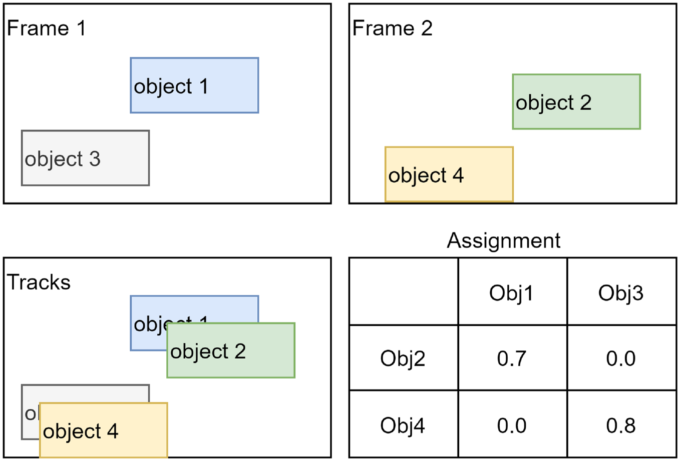
The basic concept for the intersection over union (IOU) tracker. Based on the IOU, Objects 1 and 2 in the two subsequent frames: Frames 1 and 2 represent the same track (Track 1), whereas Objects 3 and 4 represent Track 2.

Although greedy versions of IOU tracking achieve reasonable performance in some cases, they are greatly affected by false positive and false negative cases. False positive cases, for instance, may result in creating noisy and very short tracks that do not represent actual objects. Furthermore, the gaps produced by false negative examples can cause some tracks to be divided into two or more tracks (fragmented tracks). To solve such problems, we used an extended approach suggested by Erik Bochinski et al. ( 32 ). Instead of using a greedy approach for track assignment, we used the Hungarian algorithm to produce near optimal tracks. At each frame, the IOU between the last tracked position of the object and all the detections that have a confidence score above ( $σ_{l}$ ) is calculated then the Hungarian algorithm associates the detection with the corresponding track. In addition, and to solve the problems associated with false positive examples, the algorithm removes tracks that are below a certain length, $t_{\min}$ . It also remove tracks if they do not contain objects satisfying a certain detection confidence threshold, $σ_{h}$ .

To deal with false negative examples, the algorithm uses an additional single-object visual tracking technique (we used a median-flow tracker in our implementation) to compensate for missing detection. If a track is initiated and no detection satisfies a certain $σ_{IOU}$ for this track, a visual tracker for this object is initiated to estimate its trajectory for a maximum of $ttl$ frames. If a new detection satisfying $σ_{IOU}$ appears before the end of the $ttl$ frames, the IOU tracker continues and the estimation by the visual tracker stops. However, the use of visual tracking is limited to gap closures in identified tracks.

It should be noted that the median-flow tracker used in this implementation did not utilize the rich image features produced by the FPN, therefore, we did not expect it to exceed the performance of some of the state-of-the art trackers. We are are currently working on an improved version of this tracker, the discussion of which is outside the scope of this paper.

Experimentation and Results

Dataset

The dataset used for training, validation, and testing in object detection and tracking was the VisDrone2019 dataset (AISKYEYE, Tianjin University, China) ( 43 ). Different models of drones with onboard cameras were used to collect the data from 14 different cities in China that included both urban and country environments. The annotated images and videos were captured and recorded under diverse weather and lighting conditions. The dataset consists of 288 video clips formed by 261,908 frames and 10,209 static images; 2.6 million bounding boxes of targets were manually annotated by the AISKYEYE team and these targets included 10 classes of interest, namely, person, pedestrian (a human who is standing or walking on a road), car, van, bus, truck, motorcycle, bicycle, awning-tricycle, and tricycle, and each object has a corresponding confidence score. In our implementation, we focused on these images and video sequences that contained vehicles, including cars, vans, trucks, and buses. Images that contained only pedestrians, bicycles, and so forth were excluded.

For the purpose of our application in traffic analysis, we used annotated bounding boxes of the four vehicle classes: car, van, truck, and bus. In addition, the object detection models were trained on those objects with a confidence score of 1. Images used for object detection training had a height that ranged from 360 to 1,500 pixels (an average height of 1,006 pixels). The width of the training images ranged from 480 to 2,000 pixels (an average width of about 1,525 pixels). The vehicle counts of the classes in the training images are shown in Figure 5. The total number of classes (C) was five (four vehicle types plus the background).

Figure 5.

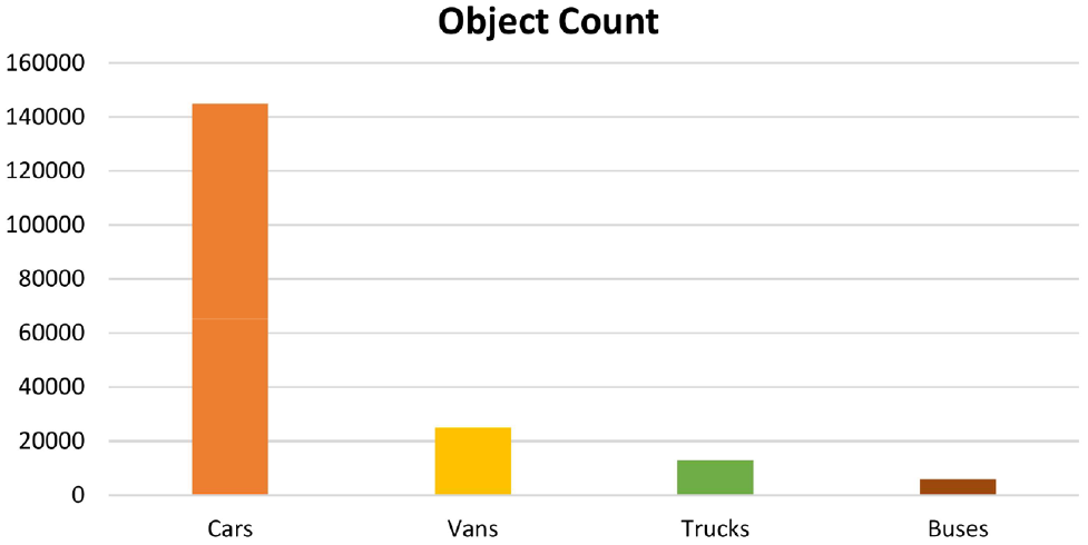
Vehicle count of the training dataset.

Model Implementation

The final extended model used a ResNet-101-FPN (FPN based on the ResNet architecture) to extract the feature pyramid, using five feature maps. The output of the FPN was then used as an input to the head RPN. The sizes and ratios used for the RPN anchor boxes were [16, 32, 64, 128, 256] and [0.5, 1., 2.0], respectively. The number of anchor boxes (N_achor) was 15. The RPN had a 3 × 3 convolution filter followed by two 1 × 1 convolution layers for objectness predictions and boundary box regression. The dimension of the classifier output was (C [number of classes]*N_achor [number of anchor boxes]), which was 5*15 in our implementation, and the dimension of the regressor output was (C*N_achor*4), where the number 4 represented the offset values for each anchor box. The four offset numbers represented the offset in the center coordinates (two values), the height of the ROI, and the width of the ROI.

The 12,000 top-scoring region proposals (only 6,000 during inference) were selected to undergo the NMS phase with an IOU threshold of 0.7. Among them, a maximum of 2,000 top-scoring regions (only 1,000 during inference) were selected as the final region proposals. Selected proposals were then used to crop the corresponding features in the feature pyramid, representing the objects to be classified. These cropped segments were scaled to a fixed sized of (14 × 14 × the number of channels) using bilinear interpolation. A max pooling layer with a 2 × 2 kernel was used to get the final (7 × 7 × the number of channels) feature map that represented the feature maps of the proposed regions. These feature maps were then fed to the classifier and bounding box regressor network branches to produce the first stage predictions of the detected objects. As mentioned earlier, the classifier produces labels for the regions whose IOUs with ground truth bounding boxes exceed a certain threshold (0.5 for the first stage). The output of the first stage was then fed to the second stage for a second-stage classification. Cascade R-CNN has a total of four detection stages; the IOU thresholds used for these stages were [0.5, 0.5, 0.6, 0.7] respectively.

Baseline Models for Assessing the Performance

We implemented two other detection models as baseline models for assessing the presented model’s performance. The first model used the SSD technique ( 19 ), which detects multiple objects using a single deep neural network. The technique is fairly powerful and produces results that are comparable to the most accurate two-stage detectors. It is commonly used in object detection applications and provided a good reference to assess the performance of the presented method. The second model was the basic Faster R-CNN architecture, which illustrates, to some extent, the impact of adding the FPN and Cascade R-CNN extensions. The following subsections discuss our implementation of the two models.

SSD

The architecture of the SSD has two main blocks: (1) the feature extraction network, which is a pretrained network (truncated before classification layers); and (2) an auxiliary structure that allows the detection and classification at multiple scales. In our implementation, we used feature extraction network VGG16 ( 44 ). For the implementation of the auxiliary structure, we used the same SSD300 model described in research from Simonyan and Zisserman ( 44 ), which uses six feature maps. Six layers ( conv4_3, conv7, conv8_2, conv9_2, conv10_2, and conv11_2) were used to predict both bounding boxes and confidence scores for each feature map.

The main change in our implementation was the dimension of input image. Rather than using 300 × 300 input images, we used a 600 × 600 input to help with the recognition of small objects. This change in the input size consequently changed the sizes of the prediction layers Conv4_3, Conv7, Conv8_2, Conv9_2, Conv10_2, and Conv11_2 to be (75, 75), (38, 38), (19, 19), (10, 10), (8, 8), (6, 6), respectively. The set of scales of the default anchor boxes used in the six feature maps was defined as [0.04, 0.10, 0.3, 0.51, 0.69, 0.87, 1.05].

Basic Faster R-CNN Model

The basic Faster R-CNN model uses VGG16 as a base network to extract the feature map. Feature maps were fed to the RPN to provide an initial region proposal and determine the objectness score of each region. The anchor box sizes and ratios in our implementation were [16, 32, 64, 128, 256] and [1, 0.7071, 1.4142] respectively. The proposed regions then pushed to an NMS phase with an IOU threshold of 0.7 and a maximum number of 600 bounding boxes. Region proposals were then used to crop the corresponding features in the feature map. An ROI pooling layer was then used to produce a fixed sized (7 × 7 × the number of channels) feature map that represented the object to be classified. Feature maps were then used to train the classifier and bounding box regressor network branches to produce the final predictions for the detected objects. The IOU threshold for the classifier was 0.4.

Evaluation Results

The model was evaluated to assess its (1) detection precision and recall, (2) ability to be used in multiobject tracking applications, and (3) ability to be used in counting applications. The results of our evaluation are presented in the following subsections.

Vehicle Detection Results

The three models were trained using a set of 6,192 images. The set was split using an 80/20 ratio, resulting in a training set of 4,960 images and a validation set of 1,232 images. We evaluated the detection performance using a test dataset of 1,534 images (images from the original set that contained at least two vehicles). The models were developed using TensorFlow (version 1.15.0) and Keras (version 2.1.5) libraries. The graphics processing unit used in the training process was an Nvidia Quadro RTX5000, which has a 16 GB memory.

To confirm whether an object was classified correctly, we needed to identify the associated ground truth bounding box. This was done by specifying a minimum IOU between the detected object and the ground truth object. If the IOU was greater than the given threshold, the object was classified as true positive, otherwise it was false positive. In our analysis, we followed the evaluation protocol used in the VisDrone challenge ( 45 ), which is very similar to the protocol used in the COCO Detection Challenge ( 16 ). In this protocol, four metrics were used to calculate the mean average precision across all classes: $A P^{IOU = 0.5 : 0.95}$ , the mean average precision over 10 IOU thresholds starting at 0.5 and ending 0.95 using a step of 0.05; $A P^{IOU = 0.5}$ , the mean average precision when the IOU with ground truth was selected to be greater than 0.5; and $A P^{IOU = 0.75}$ , the mean average precision when the IOU with ground truth was selected to be greater than 0.75.

The protocol defines mean average recall using four metrics. Across all the metrics, recall was averaged over all classes and 10 IOU values (starting from 0.5 up to 0.95 using steps of 0.05). In these metrics, the protocol limited the maximum number of detections per image. These metrics were $A R^{\max = 1}$ , the average recall given a maximum of 1 detection per image; $A R^{\max = 10}$ , the average recall given a maximum of 10 detections per image; $A R^{\max = 100}$ , the average recall given a maximum of 100 detections per image; and $A R^{\max = 500}$ , the average recall given a maximum 500 detections per image.

The test results are given in Table 1. The model built using the FPN and Cascade R-CNN achieved better results across all the metrics used in the evaluation. On the training data (not shown in the table), the model achieved average precisions of 29.98%, 53.44%, 29.61% using the $A P^{IOU = 0.5 : 0.95}$ , $A P^{IOU = 0.5}$ , and $A P^{IOU = 0.75}$ metrics, respectively. The model achieved average recalls of 1.15%, 11.38%, 34.67%, and 34.72% for $A R^{\max = 1}$ , $A R^{\max = 10}$ , $A R^{\max = 100}$ and $A R^{\max = 500}$ , respectively.

Table 1.

Detection Test Results

Model	AP ^{IOU=0.5:0.95 (%)}	AP ^{IOU=0.5 (%)}	AP ^IOU=0.75 ^(%)	AR ^max=1 ^(%)	AR ^max=10 ^(%)	AR ^max=100 ^(%)	AR ^max=500 ^(%)
Basic Faster R-CNN	2	6.88	0.44	0.65	2.99	5.43	5.43
SSD	11.98	20.75	12.78	1.25	8.91	15.09	15.09
Cascade R-CNN + FPN	20.46	38.58	18.83	1.32	11.32	25.82	25.84

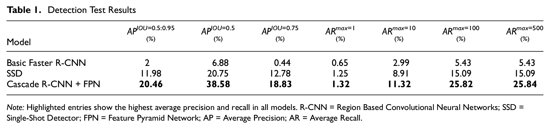
Note: Highlighted entries show the highest average precision and recall in all models. R-CNN = Region Based Convolutional Neural Networks; SSD = Single-Shot Detector; FPN = Feature Pyramid Network; AP = Average Precision; AR = Average Recall.

To get better insights on the performance of the models when used to detect different vehicle categories, we calculated $A P^{IOU = 0.5}$ and $A R^{\max = 500}$ , using the test dataset, for each of the four classes. The results are shown in Table 2. The Cascade R-CNN + FPN model achieved an $A P^{IOU = 0.5}$ of 59.78%, 21.43%, 21.14%, and 39.75% for the classes of cars, vans, trucks, and buses, respectively. The $A R^{\max = 500, IOU = 0.5}$ for the four classes, using the Cascade R-CNN + FPN, were 64.05%, 26.91%, 28.32%, and 42.99% for cars, vans, trucks, and buses respectively. The relatively good performance in car detection was expected given the large number of examples available, as indicated in Figure 5. However, model performance was relatively poor when detecting vans (misclassified as cars in many cases). Although our model implemented a weighted loss function to balance the dataset, van and truck features were not as distinguishable given the limited variation in their training examples. Buses, conversely, achieved relatively good results despite the small number of training examples because their features are easier to learn and generalize.

Table 2.

Detection Test Results Per Class

Model	AP ^Car,IOU=0.5 ^(%)	AP ^Van,IOU=0.5 ^(%)	AP ^{Truck,IOU=0.5} ^(%)	AP ^Bus,IOU=0.5 ^(%)
Basic Faster R-CNN	12.9	2.08	2.57	6.44
SSD	43.5	10.52	1.63	10.55
Cascade R-CNN + FPN	59.78	21.43	21.14	39.75
DPNet-ensemble ( 46 )	51.53	39.80	30.66	38.45
RRNet ( 46 )	51.43	36.14	35.22	44.20
ACM-OD ( 46 )	52.69	38.93	33.19	41.39

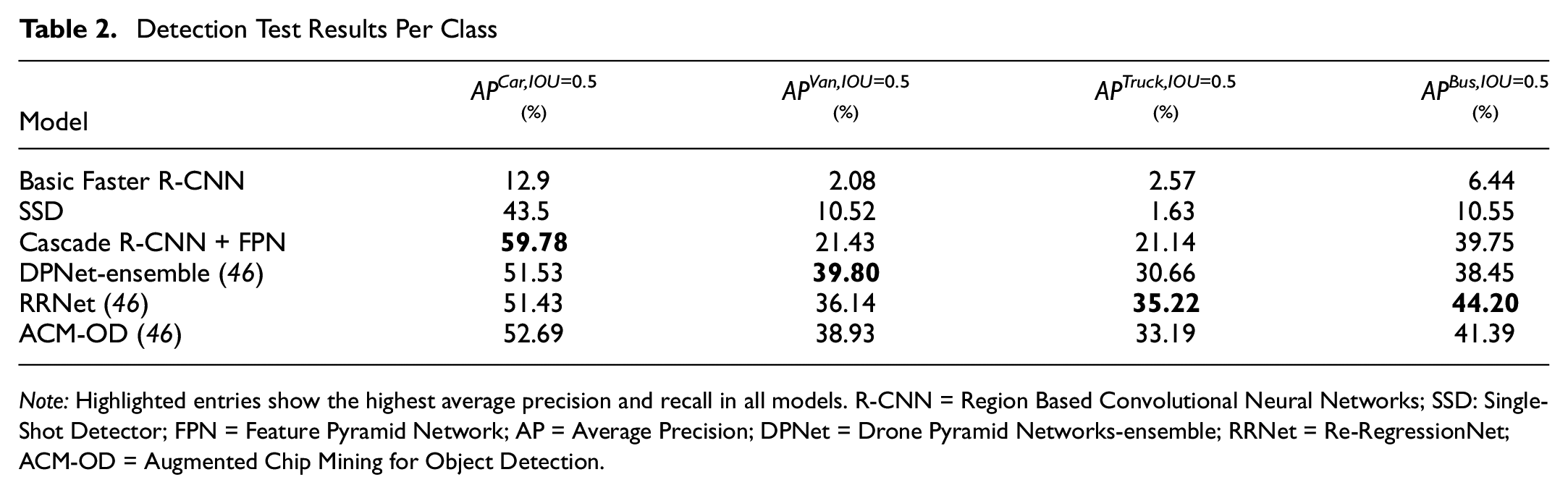
Note: Highlighted entries show the highest average precision and recall in all models. R-CNN = Region Based Convolutional Neural Networks; SSD: Single-Shot Detector; FPN = Feature Pyramid Network; AP = Average Precision; DPNet = Drone Pyramid Networks-ensemble; RRNet = Re-RegressionNet; ACM-OD = Augmented Chip Mining for Object Detection.

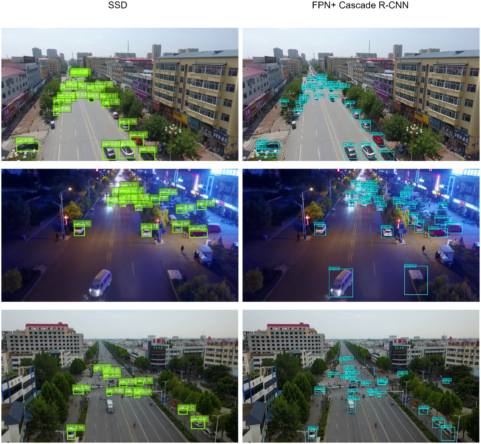
The SSD model achieved an $A R^{\max = 500, IOU = 0.5}$ of 48.08%, 13.27%, 2.44%, and 11.83% for the classes of cars, vans, trucks, and buses. The $A R^{\max = 500, IOU = 0.5}$ for the Faster R-CNN model were 21.18%, 3.65%, 15.84%, and 18.18%. Samples of the results are shown in Figure 6.

Figure 6.

Samples of the detection results.

Comparing the performance of the presented model with the top three models reported in the VisDrone dataset ( 46 ), we found that the presented model achieved better results classifying cars. However, the model had poorer performance when classifying vans, trucks, and buses. It should be noted that we did not compare the mean average precision and mean average recall (presented in Table 1) since the reported results for the top three models were calculated for the 10 classes in the VisDrone dataset (pedestrian, person, car, van, bus, truck, motor, bicycle, awning-tricycle, and tricycle), whereas our results were calculated for only four of the classes, as indicated earlier.

Multiobject Vehicle Tracking Results

Tracking performance was evaluated using the protocol used in VisDrone2019 multiobject tracking ( 47 ). This was based on the protocol suggested by the Large Scale Visual Recognition Challenge ( 48 ). The tracker algorithm extracts tracks from 14 video sequences provided by the VisDrone2019 dataset.

Tracking evaluation is not straightforward. For each ground truth track, the evaluation algorithm needs to identify the corresponding track from the set of tracklets produced by the model. In the protocol we used, the evaluation algorithm sorted all tracklets produced by the model using the average confidence of their bounding box detections. The selected tracklets were considered correct if their IOU overlap with the ground truth track was larger than a certain threshold. The protocol used three thresholds for this analysis: 0.25, 0.50, and 0.75. The mean average precision ( $mAP$ ) was calculated for the four vehicle classes over the three IOU thresholds indicating the overall performance of the algorithm.

The IOU tracker with the median-flow tracking extension was tested using the detection results from the SSD and Cascade R-CNN + FPN models. For the SSD model, we used the values of 0.3, 0.38, 23, 0.1, and 8 for the parameters of $σ_{l}$ , $σ_{h}$ , $t_{\min}$ , $σ_{IOU}$ , and $ttl$ respectively. For the Cascade R-CNN + FPN model, we used the values of 0.6, 0.68, 23, 0.1, and 8 for the same set of parameters ( $σ_{l}$ , $σ_{h}$ , $t_{\min}$ , $σ_{IOU}$ , and $ttl$ respectively). The reason for changing the values of $σ_{l}$ , $σ_{h}$ in the Cascade R-CNN + FPN model was the relatively improved performance of the model’s detections (compared to SSD), which allowed for choosing higher confidence levels. Results of the tracking evaluation are presented in Table 3.

Table 3.

Tracking Results

Model	AP ^IOU=0.25 (%)	AP ^IOU=0.5 (%)	AP ^IOU=0.75 (%)	mAP (%)
SSD	29.13	16.34	4.08	16.52
Cascade R-CNN + FPN	44.76	30.38	10.40	28.51

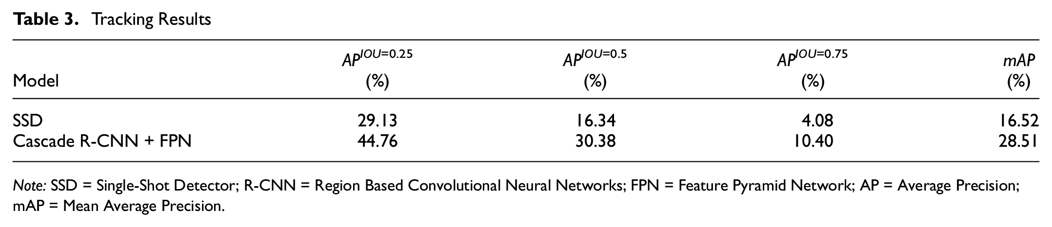
Note: SSD = Single-Shot Detector; R-CNN = Region Based Convolutional Neural Networks; FPN = Feature Pyramid Network; AP = Average Precision; mAP = Mean Average Precision.

We also evaluated the mean average precision, $AP$ , for each vehicle category. The results are shown in Table 4. SSD achieved an $A P_{car}$ of 34.56, an $A P_{van}$ of 10.65, an $A P_{truck}$ of 3.94, and an $A P_{bus}$ of 16.92. The Cascade R-CNN + FPN model achieved an $AP$ of 34.66, 27.72, 19.27, and 28.10 for cars, vans, trucks, and buses respectively. The results for the vans, trucks, and buses were expected given that tracking-by-detection algorithms rely heavily on the quality of the detections. It was surprising, however, that the performance was almost the same (34.56 in case of SSD and 34.66 in case of Cascade R-CNN + FPN) for cars, despite there typically being a significant difference between the detection performance in the two models. A possible explanation for this result is the ability of the visual tracker (median-flow extension) to compensate for missing detections. Another possible reason is that the Cascade R-CNN + FPN model detects vehicles that are not necessarily marked in the ground truth annotations (because these vehicles are very far away for instance). These posited reasons will be discussed in more detail in the vehicle counting section.

Table 4.

Tracking Results Per Class

Model	AP ^Car,IOU=0.5 (%)	AP ^Van,IOU=0.5 (%)	AP ^{Truck,IOU=0.5} (%)	AP ^Bus,IOU=0.5 (%)
SSD	34.56	10.65	3.94	16.92
Cascade R-CNN + FPN	35.09	26.18	18.20	34.58
DBAI-Tracker ( 49 )	55.13	45.85	42.73	44.97
TrackKITSY ( 49 )	54.92	41.20	34.19	29.05
Flow tracker ( 49 )	48.44	31.56	29.50	26.19

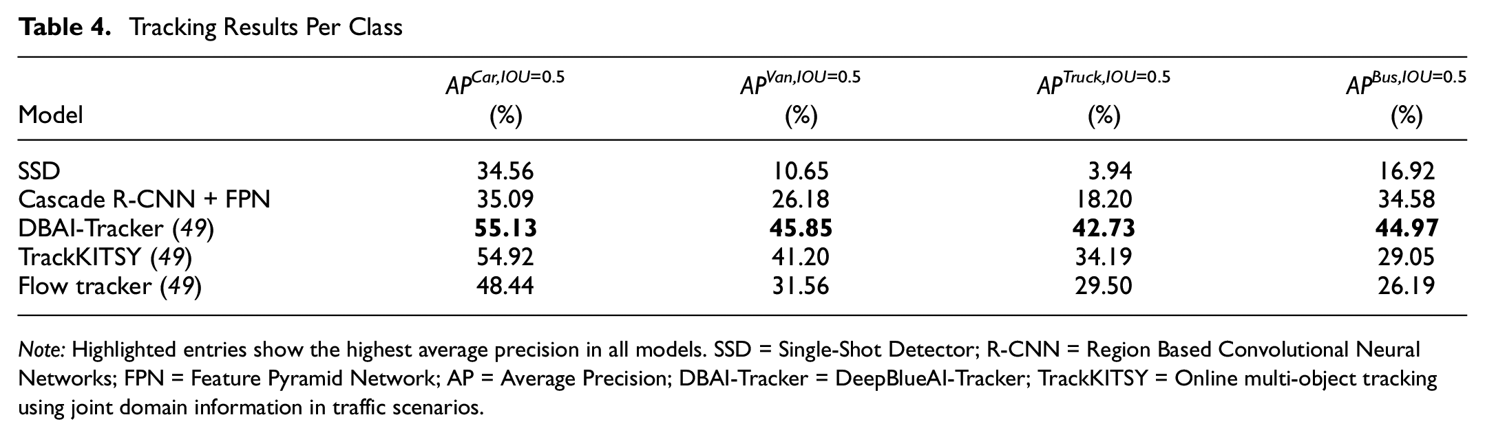
Note: Highlighted entries show the highest average precision in all models. SSD = Single-Shot Detector; R-CNN = Region Based Convolutional Neural Networks; FPN = Feature Pyramid Network; AP = Average Precision; DBAI-Tracker = DeepBlueAI-Tracker; TrackKITSY = Online multi-object tracking using joint domain information in traffic scenarios.

Comparing the performance of our model with the best reported performance of the VisDrone2019 dataset, we found that the model achieved a lower performance across all classes. This was anticipated since we were using a simple median-flow tracker that did not utilize the rich features provided by the FPN, unlike the deep blue tracker (DBAI-Tracker), for instance. As mentioned earlier, we are working on an improved version of this tracker.

Vehicle Counting Results

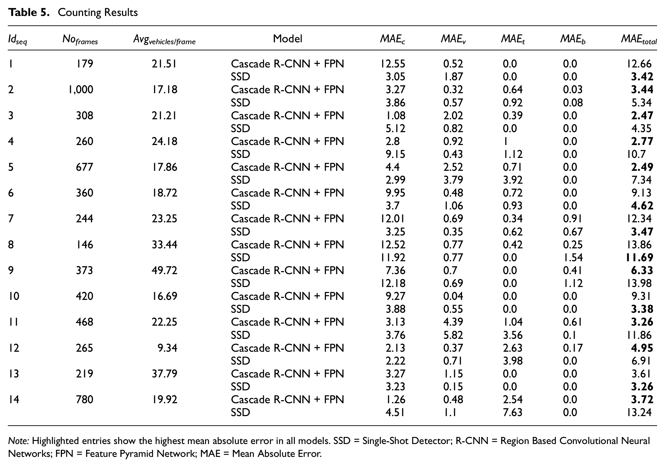
We also assessed the performance of the model when used to count vehicles by employing the 14 video sequences from the VisDrone2019 dataset. The model counted the number of unique IDs produced by trackers for the cars, vans, trucks, and buses that appeared in each frame of the VisDrone2019 MOT test sequences. For n frames within a sequence, $y_{i}$ is the count of all objects in the ground truth unique IDs in frame I, and $x_{i}$ is the count of all predicted objects in frame i as calculated from the model tracklets. The mean absolute error ( $MA E_{total}$ ) for all sequences is calculated as follows:

MA E_{total} = \frac{\sum_{i = 1}^{n} | y_{i} - x_{i} |}{n}

(2)

We also calculated $MA E_{c}$ , $MA E_{v}$ , $MA E_{t}$ , and $MA E_{b}$ for the car, van, truck, and bus objects respectively. Table 5 shows the number of frames for each sequence ( $N o_{frames}$ ), the average number of vehicles per frame ( $Av g_{vehicles / frame}$ ), the mean absolute error for each vehicle category ( $MA E_{c}$ , $MA E_{v}$ , $MA E_{t}$ , and $MA E_{b}$ ), and the total mean absolute error over all frames for the four vehicle categories. The average $MA E_{total}$ over all sequences for the SSD detector was 6.33, whereas the average $MA E_{total}$ for the Cascade R-CNN + FPN model was 6.45.

Table 5.

Counting Results

Id_seq	No_frames	Avg_{vehicles/frame}	Model	MAE_c	MAE_v	MAE_t	MAE_b	MAE_total
1	179	21.51	Cascade R-CNN + FPN	12.55	0.52	0.0	0.0	12.66
			SSD	3.05	1.87	0.0	0.0	3.42
2	1,000	17.18	Cascade R-CNN + FPN	3.27	0.32	0.64	0.03	3.44
			SSD	3.86	0.57	0.92	0.08	5.34
3	308	21.21	Cascade R-CNN + FPN	1.08	2.02	0.39	0.0	2.47
			SSD	5.12	0.82	0.0	0.0	4.35
4	260	24.18	Cascade R-CNN + FPN	2.8	0.92	1	0.0	2.77
			SSD	9.15	0.43	1.12	0.0	10.7
5	677	17.86	Cascade R-CNN + FPN	4.4	2.52	0.71	0.0	2.49
			SSD	2.99	3.79	3.92	0.0	7.34
6	360	18.72	Cascade R-CNN + FPN	9.95	0.48	0.72	0.0	9.13
			SSD	3.7	1.06	0.93	0.0	4.62
7	244	23.25	Cascade R-CNN + FPN	12.01	0.69	0.34	0.91	12.34
			SSD	3.25	0.35	0.62	0.67	3.47
8	146	33.44	Cascade R-CNN + FPN	12.52	0.77	0.42	0.25	13.86
			SSD	11.92	0.77	0.0	1.54	11.69
9	373	49.72	Cascade R-CNN + FPN	7.36	0.7	0.0	0.41	6.33
			SSD	12.18	0.69	0.0	1.12	13.98
10	420	16.69	Cascade R-CNN + FPN	9.27	0.04	0.0	0.0	9.31
			SSD	3.88	0.55	0.0	0.0	3.38
11	468	22.25	Cascade R-CNN + FPN	3.13	4.39	1.04	0.61	3.26
			SSD	3.76	5.82	3.56	0.1	11.86
12	265	9.34	Cascade R-CNN + FPN	2.13	0.37	2.63	0.17	4.95
			SSD	2.22	0.71	3.98	0.0	6.91
13	219	37.79	Cascade R-CNN + FPN	3.27	1.15	0.0	0.0	3.61
			SSD	3.23	0.15	0.0	0.0	3.26
14	780	19.92	Cascade R-CNN + FPN	1.26	0.48	2.54	0.0	3.72
			SSD	4.51	1.1	7.63	0.0	13.24

Note: Highlighted entries show the highest mean absolute error in all models. SSD = Single-Shot Detector; R-CNN = Region Based Convolutional Neural Networks; FPN = Feature Pyramid Network; MAE = Mean Absolute Error.

While the Cascade R-CNN + FPN model performed better in eight sequences (Sequences 2, 3, 4, 5, 9, 11, 12, and 14), the SSD exceeded its performance in Sequences 1, 6, 7, 8, 10, and 13. That was unexpected given the improved detection quality of the Cascade R-CNN + FPN model. After further investigation, we found that in these sequences the Cascade R-CNN + FPN detected several vehicles that were not necessarily annotated in the dataset owing to the vehicles being far away, unclear, or harder to detect. This was also the case with the SSD model, but this model detected far fewer of these vehicles. Consequently, in many frames, the number of true positive vehicles detected by Cascade R-CNN + FPN was greater than the ground truth vehicles, directly affecting the mean absolute error values. This problem is illustrated in Figure 7, which shows frames from Sequences 1 and 6, where the SSD model exceeded the performance of the Cascade R-CNN + FPN model. Vehicles that were not marked by the ground truth annotations of the dataset impaired the performance of the Cascade R-CNN + FPN model.

Figure 7.

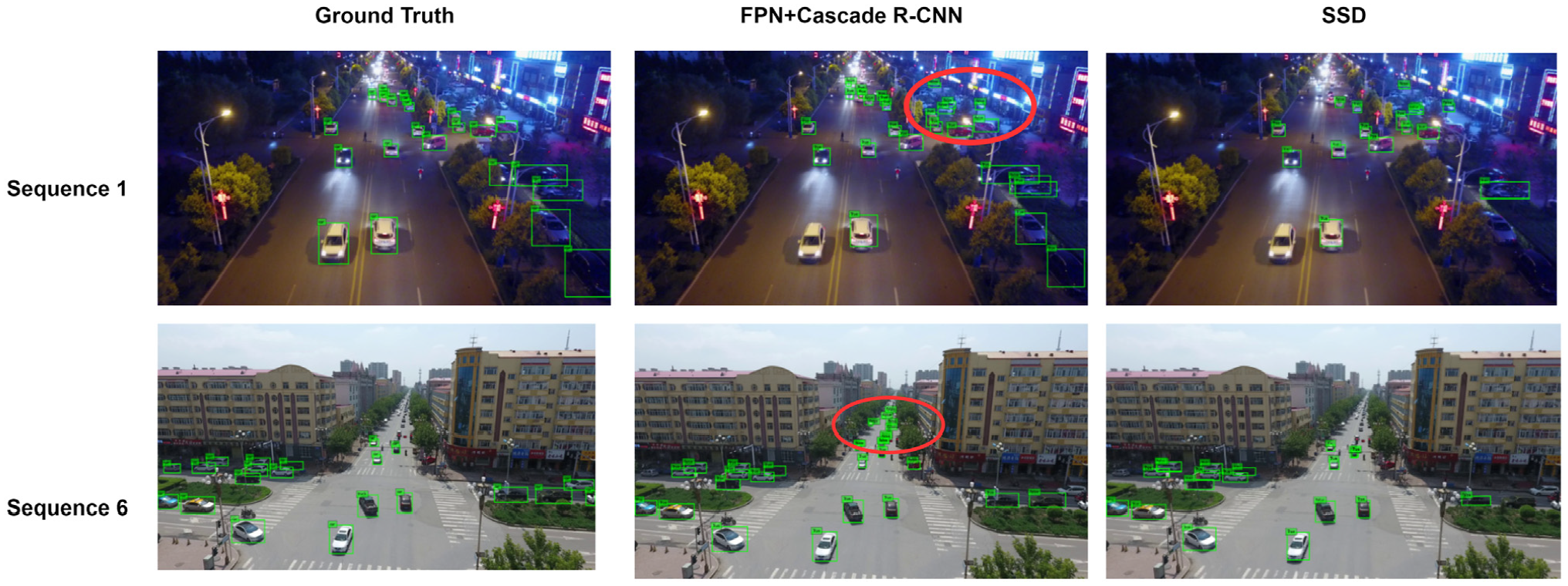
Samples of cases where ground truth annotations do not show all vehicles in the sequence images.

Conclusion

The presented work addressed the problem of vehicle detection, counting, and tracking using video feeds from UAV-mounted cameras. The approach did not require any calibration procedures, specific orientations, or specific camera viewpoints. Images can be taken from different ground sampling distances, resulting in objects that can vary greatly in shape and scale even when belonging to the same class.

We implemented a vehicle detection and classification model that used a region-based convolutional neural network to classify four types of vehicles: cars, vans, trucks, and buses. The model leveraged an FPN to extract a semantically rich feature pyramid capable of representing the different objects at multiple scales. It also used a multistage Cascade R-CNN architecture capable of producing high-quality detections that are less sensitive to IOU thresholds. The model was trained and tested using more that 6,192 images from the VisDrone2019 dataset. The model achieved an average precision of 59.78% for cars when the IOU with ground truth was greater than 0.5. The precision dropped for the other categories such as vans and trucks, resulting in an overall average precision of 20.46% for the four classes over 10 different thresholds. We believe that this drop resulted from the lack of training examples in these categories compared with the car category.

The detection model was used to build an IOU tracker that uses a tracking-by-detection paradigm. The tracker uses a median-flow tracking extension to compensate for gaps in tracks. The tracker was tested by using it to extract tracks from 14 sequences in the VisDrone2019 dataset. It achieved a mean average precision of 28.51% as compared to 16.52% when detection was performed using an SSD. The detection model was also evaluated for counting applications. Results showed that the model performed well, achieving a mean absolute error that ranged between 2.47 and 13.86. We believe accuracy was greater owing to the model detecting several vehicles that were not necessarily annotated in the dataset.

Footnotes

Acknowledgements

The authors thank Tasneem Omara and Aya Alzahy of Zewail City of Science and Technology for their valuable assistance.

Author Contributions

The authors confirm contribution to the paper as follows: study conception and design: M. Elshenawy, Y. Youssef; data collection: Y. Youssef; analysis and interpretation of results: Y. Youssef, M. Elshenawy; draft manuscript preparation: M. Elshenawy, Y. Youssef. All authors reviewed the results and approved the final version of the manuscript.

Declaration of Conflicting Interests

The authors declared no potential conflicts of interest with respect to the research, authorship, and/or publication of this article.

Funding

The authors disclosed receipt of the following financial support for the research, authorship, and/or publication of this article: This research is supported by Zewail City’s internal research fund (grant no. ZC 023-2019).

References

Dai

Wang

Learning Traffic as Images: A Deep Convolutional Neural Network for Large-Scale Transportation Network Speed Prediction. Sensors, Vol. 17, No. 4, 2017, p. 818.

Lee

Son

Kim

Park

Car Plate Recognition Based on CNN Using Embedded System with GPU. In 2017 10th International Conference on Human System Interactions (HSI), IEEE, 2017, pp. 239–241.

Kocatepe

Ulak

M. B.

Kakareko

Pinzan

Cordova

Ozguven

E. E.

Jung

Arghandeh

Sobanjo

J. O.

Assessment of Emergency Facility Accessibility in the Presence of Hurricane-Related Roadway Closures and Prediction of Future Roadway Disruptions. Presented at 97th Annual Meeting of the Transportation Research Board, Washington, D.C., 2018.

Kocatepe

Ulak

M. B.

Kakareko

Ozguven

E. E.

Jung

Arghandeh

Measuring the Accessibility of Critical Facilities in the Presence of Hurricane-Related Roadway Closures and An Approach for Predicting Future Roadway Disruptions. Natural Hazards, Vol. 95, No. 3, 2019, pp. 615–635.

Sivaraman

Trivedi

M. M.

Looking at Vehicles on the Road: A Survey of Vision-Based Vehicle Detection, Tracking, and Behavior Analysis. IEEE Transactions on Intelligent Transportation Systems, Vol. 14, No. 4, 2013, pp. 1773–1795.

Elshenawy

El-darieby

Abdulhai

Automatic Imputation of Missing Highway Traffic Volume Data. In 2018 IEEE International Conference on Pervasive Computing and Communications Workshops (PerCom Workshops), 2018, pp. 373–378.

Kanistras

Martins

Rutherford

M. J.

Valavanis

K. P.

A Survey of Unmanned Aerial Vehicles (UAVs) for Traffic Monitoring. In 2013 International Conference on Unmanned Aircraft Systems (ICUAS), IEEE, 2013, pp. 221–234.

Shakhatreh

Sawalmeh

A. H.

Al-Fuqaha

Dou

Almaita

Khalil

Othman

N. S.

Khreishah

Guizani

Unmanned Aerial Vehicles (UAVs): A Survey on Civil Applications and Key Research Challenges. IEEE Access, Vol. 7, 2019, pp. 48572–48634.

Khan

M. A.

Ectors

Bellemans

Janssens

Wets

Unmanned Aerial Vehicle–Based Traffic Analysis: Methodological Framework for Automated Multivehicle Trajectory Extraction. Transportation Research Record: Journal of the Transportation Research Board, 2017. 2626: 25–33.

10.

Barmpounakis

E. N.

Vlahogianni

E. I.

Golias

J. C.

Extracting kinematic characteristics from unmanned aerial vehicles. Presented at 95th Annual Meeting of the Transportation Research Board, Washington, D.C., 2016. .

11.

Chow

J. Y.

Dynamic UAV-Based Traffic Monitoring under Uncertainty as a Stochastic Arc-Inventory Routing Policy. International Journal of Transportation Science and Technology, Vol. 5, No. 3, 2016, pp. 167–185.

12.

Braut

Čuljak

Vukotić

Šegvić

Ševrović

Gold

Estimating OD Matrices at Intersections in Airborne Video-a Pilot Study. Proc., 35th International Convention MIPRO, IEEE, 2012, pp. 977–982.

13.

Barmpounakis

E. N.

Vlahogianni

E. I.

Golias

J. C.

, Unmanned Aerial Aircraft Systems for Transportation Engineering: Current Practice and Future Challenges. International Journal of Transportation Science and Technology, Vol. 5, No. 3, 2016, pp. 111–122.

14.

Papageorgiou

Poggio

A Trainable System for Object Detection. International Journal of Computer Vision, Vol. 38, No. 1, 2000, pp. 15–33.

15.

Zhang

Ren

Sun

Deep Residual Learning for Image Recognition. Proceedings of the IEEE Conference on Computer Vision and Pattern Recognition, 2016, pp. 770–778.

16.

Hosang

Benenson

Dollár

Schiele

What Makes for Effective Detection Proposals?

IEEE Transactions on Pattern Analysis and Machine Intelligence, Vol. 38, No. 4, 2015, pp. 814–830.

17.

Deng

Dong

Socher

L.-J.

Fei-Fei

Imagenet: A Large-Scale Hierarchical Image Database. In 2009 IEEE Conference on Computer Vision and Pattern Recognition, IEEE, 2009, pp. 248–255.

18.

Redmon

Divvala

Girshick

Farhadi

You Only Look Once: Unified, Real-Time Object Detection. In Proceedings of the IEEE Conference on Computer Vision and Pattern Recognition, 2016, pp. 779–788.

19.

Liu

Anguelov

Erhan

Szegedy

Reed

C.-Y.

Berg

A. C.

SSD: Single Shot Multibox Detector. In European Conference on Computer Vision, Springer, 2016, pp. 21–37.

20.

Long

Shelhamer

Darrell

Fully Convolutional Networks for Semantic Segmentation. In Proceedings of the IEEE Conference on Computer Vision and Pattern Recognition, 2015, pp. 3431–3440.

21.

Ren

Girshick

Sun

Faster R-CNN: Towards Real-Time Object Detection with Region Proposal Networks. In Advances in Neural Information Processing Systems, 2015, pp. 91–99.

22.

Gkioxari

Dollár

Girshick

. Mask R-CNN. In Proceedings of the IEEE International Conference on Computer Vision, 2017, pp. 2961–2969.

23.

Liang

Song

Dai

Vehicle Counting System Using Deep Learning and Multi-Object Tracking Methods. Transportation Research Record: Journal of the Transportation Research Board, 2020. 2674: 114–128.

24.

Dai

Song

Wang

Fang

Yun

Zhang

Video-based Vehicle Counting Framework. IEEE Access, Vol. 7, 2019, pp. 64460–64470.

25.

Zhang

Costeira

J. P.

Moura

J. M.

FCN-rLSTM: Deep Spatio-Temporal Neural Networks for Vehicle Counting in City Cameras. In Proceedings of the IEEE International Conference On Computer Vision, 2017, pp. 3667–3676.

26.

Onoro-Rubio

López-Sastre

R. J.

Towards perspective-free object counting with deep learning. In European Conference on Computer Vision, Springer, 2016, pp. 615–629.

27.

Awang

Azmi

N. M. A. N.

Vehicle Counting System Based on Vehicle Type Classification Using Deep Learning Method. In IT Convergence and Security 2017, Springer, 2018, pp. 52–59.

28.

Wojke

Bewley

Paulus

Simple Online and Realtime Tracking with A Deep Association Metric. In 2017 IEEE International Conference on Image Processing (ICIP), IEEE, 2017, pp. 3645–3649.

29.

Liu

Zhang

Gao

Meng

Tan

Zhu

Xue

Zhang

Wen

Ding

Robust Movement-Specific Vehicle Counting at Crowded Intersections. In Proceedings of the IEEE/CVF Conference on Computer Vision and Pattern Recognition Workshops, 2020, pp. 614–615.

30.

Lin

T.-Y.

Dollar

Girshick

Hariharan

Belongie

Feature Pyramid Networks for Object Detection. In Proceedings of the IEEE Conference on Computer Vision and Pattern Recognition (CVPR), 2017, pp. 2117–2125.

31.

Cai

Vasconcelos

Cascade R-CNN: Delving Into High Quality Object Detection. In Proceedings of the IEEE Conference on Computer Vision and Pattern Recognition (CVPR), 2018, pp. 3361–369.

32.

Bochinski

Senst

Sikora

Extending IOU Based Multi-Object Tracking by Visual Information. In 2018 15th IEEE International Conference on Advanced Video and Signal Based Surveillance (AVSS), IEEE, 2018, pp. 1–6.

33.

Yang

Real-Time Vehicle Detection and Counting in Complex Traffic Scenes Using Background Subtraction Model with Low-Rank Decomposition. IET Intelligent Transport Systems, Vol. 12, No. 1, 2017, pp. 75–85.

34.

Abdelwahab

Fast Approach for Efficient Vehicle Counting. Electronics Letters, Vol. 55, No. 1, 2018, pp. 20–22.

35.

Krizhevsky

Sutskever

Hinton

G. E.

Imagenet Classification with Deep Convolutional Neural Networks. Communications of the ACM, Vol. 60, No. 6, 2017, pp. 84–90.

36.

Zhang

Ren

Sun

Spatial Pyramid Pooling in Deep Convolutional Networks for Visual Recognition. IEEE Transactions on Pattern Analysis and Machine Intelligence, Vol. 37, No. 9, 2015, pp. 1904–1916.

37.

Zhang

Lin

Liang

Is Faster R-CNN Doing Well for Pedestrian Detection? In European Conference on Computer Vision, Springer, 2016, pp. 443–457.

38.

Saleh

Hossny

Nahavandi

Cyclist Detection in Lidar Scans Using Faster r-CNN and Synthetic Depth Images. In 2017 IEEE 20th International Conference on Intelligent Transportation Systems (ITSC), IEEE, 2017, pp. 1–6.

39.

Kalman

R. E.

A New Approach to Linear Filtering and Prediction Problems. Journal of Basic Engineering, Vol. 82, No. 1, 1960, pp. 35–45.

40.

Wang

A Multiple Object Tracking Method Using Kalman Filter. In The 2010 IEEE International Conference on Information and Automation, IEEE, 2010, pp. 1862–1866.

41.

Ciaparrone

Sánchez

F. L.

Tabik

Troiano

Tagliaferri

Herrera

Deep Learning in Video Multi-Object Tracking: A Survey. Neurocomputing, Vol. 381, 2020, pp. 61–88.

42.

Bewley

Ott

Ramos

Upcroft

Simple Online and Realtime Tracking. In 2016 IEEE International Conference on Image Processing (ICIP), IEEE, 2016, pp. 3464–3468.

43.

Zhu

Wen

Bian

Haibin

Vision Meets Drones: A Challenge. arXiv preprint arXiv:1804.07437, 2018.

44.

Simonyan

Zisserman

, Very Deep Convolutional Networks for Large-Scale Image Recognition. arXiv preprint arXiv:1409.1556, 2014.

45.

Object Detection Evaluation , 2020. http://aiskyeye.com/evaluate/object-detection/Accessed: January 20, 2021.

46.

Zhu

Wen

Bian

Lin

Peng

Zheng

Wang

Zhang

Shi

Zhu

Kumar

Zinollayev

Askergaliyev

Schumann

Mao

Lee

Liu

Chen

Pan

Huo

Cong

Zeng

Pailla

D. R.

Wang

Cho

Zhang

Bai

Jose

Gao

Liu

Xiong

Wang

Qiu

Kim

Shen

Lee

Zhou

Meier

Choi

J. W.

Zhang

Huang

Wang

Sommer

Jin

Zhang

Huang

Sun

Steinmann

Jia

Zhang

Chen

Liu

Cheng

Chennamsetty

Chen

Wei

Kruthiventi

Hong

Kang

Feng

Kollerathu

V. A.

Dai

Qin

Wang

Chen

Sun

Zhang

Zhao

Zhang

Chen

Wei

Zhang

Chen

Toh

Y. H.

Zhang

Zhu

Zhong

Wang

Song

Liu

. VisDrone-DET2019: The Vision Meets Drone Object Detection in Image Challenge Results. In 2019 IEEE/CVF International Conference on Computer Vision Workshop (ICCVW), 2019.

47.

Multi-Object Tracking Evaluation, 2020. http://aiskyeye.com/evaluate/multi-object-tracking/, Accessed: January 20, 2021.

48.

Park

Liu

Russakovsky

Deng

F.-F.

Berg

Large Scale Visual Recognition Challenge 2017, 2017.

49.

Wen

Zhu

Bian

Ling

Zheng

Peng

Wang

Zhang

Shi

Zhu

Jadhav

Dong

Lall

Liu

Zhang

Wang

Bunyak

Wang

Liu

Seetharaman

Ardo

Zhang

Hwang

Palaniappan

Chen

Ding

Lauer

Nilsson

Al-Shakarji

Mukherjee

Huang

Laganiere

Chen

Pan

Kaushik

Shi

Tian

Chen

Zhang

Zhao

Wang

Song

Yao

Chen

Xiao

Tong

Luo

Sun

. Visdrone-mot2019: The vision meets drone multiple object tracking challenge results. In Proceedings of the IEEE International Conference on Computer Vision Workshops, 2019.

Automatic Vehicle Counting and Tracking in Aerial Video Feeds using Cascade Region-based Convolutional Neural Networks and Feature Pyramid Networks

Abstract

Related Work

Methodology

Vehicle Detection and Classification

Faster R-CNN Architecture

The Detection Model

FPN

Cascade R-CNN

Multiobject Vehicle Tracking Module

Experimentation and Results

Dataset

Model Implementation

Baseline Models for Assessing the Performance

SSD

Basic Faster R-CNN Model

Evaluation Results

Vehicle Detection Results

Multiobject Vehicle Tracking Results

Vehicle Counting Results

Conclusion

Footnotes

Acknowledgements

Author Contributions

Declaration of Conflicting Interests

Funding

References