
Abstract
We present a methodology to extract points of interest (POIs) data from OpenStreetMap (OSM) for application in travel demand models. We use custom taglists to identify and assign POI elements to typical activities used in travel demand models. We then compare the extracted OSM data with official sources and point out that the OSM data quality depends on the type of POI and that it generally matches the quality of official sources. It can therefore be used in travel demand models. However, we recommend that plausibility checks should be done to ensure a certain quality. Further, we present a methodology for calculating attractiveness measures for typical activities from single POIs and national trip generation guidelines. We show that the quality of these calculated measures is good enough for them to be used in travel demand models. Using our approach, therefore, allows the quick, automated, and flexible generation of attractiveness measures for travel demand models.
Travel demand models are an essential tool for estimating the traffic effects of infrastructural changes. Today, travel demand models are usually created manually. For this purpose, data from the network along with supply and structural data are collected from all participating offices and authorities. By structural data we mean statistics and information that are highly spatial, such as, the distribution of age or gender in an area. Additionally, data about behavior are collected by using existing travel surveys or conducting new ones. A traffic engineer can merge the data and fix errors and inconsistencies. In the subsequent calibration process, the model is adapted to reality to be able to draw valid conclusions. The data play a crucial role in this process as they form the basis of all further findings and results. The data have to be as valid as possible to support the findings. Thus, a large part of the time in this process is taken up by the collection and preparation of the data.
Following typical approaches in travel demand modeling, several decisions are made by individuals and are therefore represented in the models, the most important being: which activities should be conducted; where should the activity happen; and which mode and which route should be used to move to the activity location ( 1 ). Looking more closely at location choice, one can see that individuals make destination decisions every day. People are looking for feasible destinations to satisfy a certain need: supermarkets allow people to take care of their weekly grocery purchases; local recreation areas serve as places for spending leisure time; and train stations are appropriate points for picking up or dropping off friends or relatives. Consequently, the structure of an area determines its attractiveness as a destination for different purposes. Travel demand models use attractiveness as a measure to model people’s destination choices by using spatial interaction models ( 2 ). For this purpose, structural data, such as the sales area of retail facilities or the daily number of visitors to recreational facilities, are collected. The structural data can afterwards be used as one term in destination choice models representing the static attraction of a destination or traffic analysis zone.
Instead of collecting and preparing the data manually, the spatial data can also be purchased from data service providers such as HERE (formerly Navteq). Those providers endeavor to provide good quality data. However, less is known about their data sources and processing. One, therefore, needs to validate the quality of the data for using them. Depending on the required amount of data being used to build a travel demand model, purchasing such data from providers can be expensive. Spatial data can be collected manually or bought from a data service provider. Either way, it is a resource-intensive task. The current trend toward open data could help here.
Generally, open data offer many advantages. Open data are provided in an open format which is typically well documented. This substantially reduces the work involved in using the data from a technical point of view. If the data are available in a uniform format for different areas, all methodologies, frameworks, and procedures built on them can be transferred to other regions more easily. Moreover, as the data are available in a defined format, they can be processed automatically in all available areas. In addition, if the data are updated regularly, all models derived from them can also be updated regularly. The openness of the data also encourages the transparency of the models derived from them. Anybody who knows the process is able to reproduce the results. Thus, there is no longer a “black box” as with purchased data.
The methodology proposed in this paper aims to reduce the time it takes to create a model and to create more transparent models by using open data. This paper is structured as follows. First, a literature review gives an overview of all relevant topics. Second, the data source is described. Third, the methodology used in collecting and processing the data is explained. Forth, the results are validated by a comparison with an other model and real-world data. Finally, the paper finishes with a conclusion and outlook for future research.
Literature Review
The most common source for spatial open data is OpenStreetMap (OSM). OSM contains data from around the world and provides it in a defined and documented way. For instance, streets and districts are modeled in the same way all over the world. Most of the data in OSM are collected and maintained by volunteers. In some countries, such as Germany or the USA, public authorities also provide data for OSM. OSM data have the advantage of being more up-to-date than data from public authorities because of the continuous maintenance by volunteers. Changes made to the dataset of OSM can be downloaded at any time. However, older versions of the data are still available. Depending on the region of interest, preprocessed data are updated once a week ( 3 ). For example, Briem et al. ( 4 ) found that locations open to the public are kept up-to-date. Changes are made on a daily basis unlike the annual statistics of public authorities where changes only appear in the next edition. Thus, in some cases, shops might be included before they are open. In contrast, locations that are not open to the public are maintained less frequently. Any assessment of workplaces is, therefore, distorted because many small offices, which are not open to the public, are missing from OSM ( 4 ). Having the data maintained by enthusiasts is an advantage in many regions, but in others it is less so, especially if there are only a few active volunteers. Therefore, the OSM data on any given area are highly dependent on the number of volunteers. In areas with many volunteers the data are better than in areas with only a few.
OSM was already used as input data for an agent-based transport simulation model by Zilske et al. ( 5 ). They used the network from OSM and showed that it provided data of sufficient quality to be used as a data source. Subsequently, Ziemke et al. ( 6 ) combined various open data sources to build up a synthetic demand based on open data. They fed the result into an agent-based transport simulation scenario for Berlin and showed that it was sufficient for this purpose. Their data generation procedure was even spatially transferable as it was not built on a local travel survey.
A current project using open data for travel demand modeling is “Transportation Modeling Using Publicly Available Data” founded by German Research Foundation (DFG). This project compares the use of open and traditional data in building up transport models. The study uses three models of regions located on different continents: Africa, America, and Europe. Their goal is to investigate: whether open data are sufficient for use as a data source; in which areas open data have drawbacks; and in which areas it is better than traditional data. This should result in a transparent process to derive a travel demand model from open data, with the findings of models being more transparent.
Those projects show that open data can provide input for travel demand models in the form of networks and behavior. The supply for different modes can be derived from OSM and other data sources. However, as well as travel modes, individuals also choose destinations. Valdes et al. ( 7 ) demonstrated the use of OSM point of interest (POI) data for estimating demand at charging stations for electric vehicles. They considered them as destinations for activities of four different types. While they showed that their approach worked in the case of electric charging, more is needed to build up a complete travel demand model.
Horni and Axhausen ( 8 ) presented an initial approach to improving destination choice for discretionary activities. This can be interpreted as the destination choice to individual POIs in microsimulations. They further mentioned a lack of available data to build such a model. Based on recent developments in data processing and technologies, Molloy and Moeckel ( 9 ) showed an approach that enhanced destination choice modeling by using big data technology. They described a methodology to collect and process check-in counts at various sights.
Most data processes today focus on directly feeding a microscopic travel demand model and ignore the geometric attributes of POIs. We address both issues in our approach. By considering the geometry of each single POI, the methodology presented can generate data either for microscopic or macroscopic travel demand models and thus allows a smooth transition from one to the other. Further, we developed a methodology to calculate typical attractiveness values from POIs. We applied the methodology in various regions in the United States and Europe and show first results for one of those regions.
Open Street Map
OSM is a open database that contains Volunteered Geographic Information (VGI) under the Open Database License. Since its foundation in London in 2004, the number of contributors has increased to over 7 million, making OSM the largest database of its kind. The map material covers the entire globe and includes features such as roads, buildings, and POIs, as well as land-use data. The OSM database consists of three basic elements (3, 10) which have unique IDs for identification.
Nodes: A node represents a point on the earth’s surface, which is defined by its latitude and longitude. In addition, each node receives a unique ID for identification.
Ways: A way is a polyline defined by between two and 2,000 referenced nodes which, for example, represent a road. Closed ways are also used to define areas, such as buildings.
Relations: For more complex structures relations are used. A relation describes the relationship between multiple elements, for example, a multipolygon can be used to represent buildings with an inner courtyard, with an outer way representing the boundary of the building and inner ways representing the courtyard.
Additional information is added to the elements by tags. Tags are a combination of a key and a value which are both arbitrary strings, for example, “shop = supermarket.” Any number of them can be attached to an OSM element. Volunteers who collect the data are free to use these tags as they wish, so no uniform scheme can be guaranteed. However, recommended input masks exist in various software applications that are used to record an element. These input masks are based on feature lists described and strongly recommended by the OSM Wiki ( 3 ). The editors of OSM maintain the list as an informal standard. Voting is used to decide which new tags should be added as map features ( 10 ). When adding new objects to OSM, the contributor decides which element type and which tags are used, for example, when adding a new shop to OSM, the contributor can define a node, a way, or a relation with the corresponding tag “shop = supermarket,” see Figure 1. A way can be defined either for an area within a building or for the building itself when the additional tag “building = *” is used. A less detailed option is a way that is defined by the tag “landuse = retail” describing a whole area where different shops and supermarkets are located.
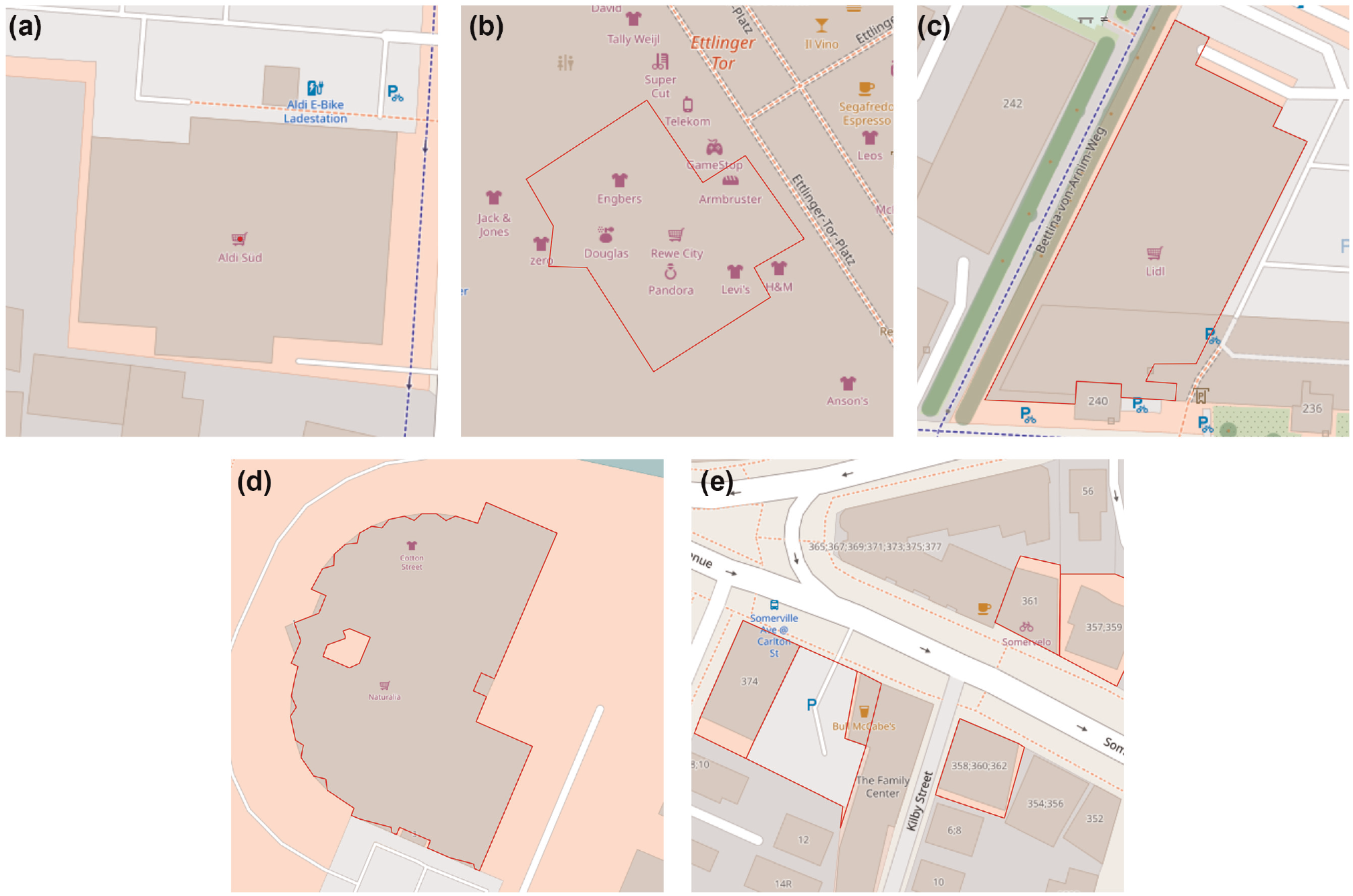
Different methods of modeling a supermarket: (a) as a node; (b) as an area within a building; (c) as a building; (d) as a relation representing a building; and (e) as an area of the land-use retail.
These various options for defining objects result in heterogeneous data, where potential POIs for transport modeling are reported as different OSM elements with more or less detail. This implies that the data must be aligned first, so that POIs can be properly categorized and valid measures of attractiveness can be created (see the section on Data Collection).
The OSM data are updated and checked by the community at different frequencies depending on the region and type of data. Worldwide, about 2 million changes are made every day. According to the company Mapbox, 0.2% of these are vandalism and 2% are of poor quality ( 11 ). However, the users and various institutions such as Mapbox ensure that 50% of the bad edits are improved on the day they are made. Several error detection and monitoring tools are in use to support the contributors ( 3 ). Providers like Mapbox offer additionally controlled OSM datasets for sale.
The validation of (spatial) input data for travel demand models is part of the quality assurance process during model development ( 12 ). In general, the quality of the data can be checked in six different categories ( 13 ): positional, thematic, and temporal accuracy; completeness; logic consistency; usability. Thematic accuracy and completeness are particularly important when using OSM data to generate POI data. The exact positional and temporal accuracy is more relevant for navigation purposes, though discrepancies should not be large. These features can be checked using intrinsic or extrinsic methods. For extrinsic approaches to examine POIs, verified and therefore suitable area-wide datasets are seldom available for comparison or they are expensive to obtain. However, random checks made by persons with local knowledge or the use of available data sources from third parties (e.g., Google Maps or the websites of local authorities) are possible and provide indications of data quality ( 4 ). For intrinsic analyses, tools are being developed by various institutions that enable historical or quantitative investigations (e.g., Ohsome [14], Is OSM up-to-date [15] or QXOSM [16]). Since individual analyses alone are of limited value, the use of frameworks is desirable ( 17 ). Most studies on the quality of OSM data are focused on extrinsic studies of the transport network, which is why there is still a need for research on the quality of POI data ( 18 ).
Methodology
The approach presented consists of two stages. First, data from OSM are gathered. The POIs—nodes, ways, and relations—are assigned to an activity type. Second, all POIs of an activity type are converted to a purpose-specific attractiveness for traffic analysis zones.
Data Collection
There are different methods used to access OSM data. We use OSM data from Geofabrik in .osm.pbf format. To work with the OSM data the tools Osmosis, JOSM, and ArcMap are used. Osmosis is an open source command line application used to process OSM data. It is built in a modular way to combine basic building blocks to larger processing chains ( 3 ). Osmosis has powerful filter capabilities, which can be used to find elements with certain tags or within a geographical region. JOSM is a tool for visualization and completion of ways and elements destroyed by spatial filters ( 3 ). ArcMap offers area calculations and other geographic data processing procedures, which can be automated in process chains.
To use the OSM data in a travel demand model, the OSM elements must be assigned to one or more activities as a first step. For this purpose, a tag list is created for each activity. The data are then filtered using the tag lists with the Osmosis software. As mentioned in the section on Open Street Map, the tags typically used are an informal standard. This allows the lists to be transferred to other cities without checking the tags that are only locally available in a city. When assigning destinations to activities, any fine-segmented activities can be used, since OSM tags are usually very specific. This is especially true for the activities “shopping,”“personal business,” and “leisure.” The reason for this is that locations where these activities can be conducted are typically open to the public and, accordingly, OSM contributors have a greater interest in the detailed recording of these destinations. To find all tags associated with an activity, the feature lists on ( 3 ) were fully analyzed and assigned to the activities. The web service taginfo ( 19 ), which was also used in the process, allows searches for frequently used tags. To consider as many tags as possible, only the key need be given and an arbitrary value is accepted (e.g., “doctor = *”). Table 1 shows an example of a tag list for the activity “shopping daily.” Similar lists were created for the other activities shown in Table 2.
Tag List for the Activity Type Shopping Daily

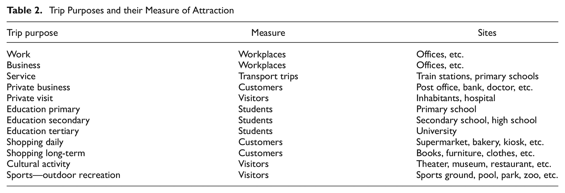
Trip Purposes and their Measure of Attraction
For many activities, it is not just the existence of the POI that is relevant, but also the degree of attractiveness, which can for example be calculated by using the number of square meters and specific parameters ( 20 ). When calculating the attractiveness, a distinction must be made between the different OSM elements described in the section on Open Street Map and the different activities. Various possible procedures for calculating the square meters are explained below.
For the ways and relations to which the tag “building” is added (for example, “building = *”) the area is calculated using the polygon of the element. If the number of floors is given as a tag, the floor area is also calculated. It is assumed that a way representing a building with tags assigning it to an activity is used for this activity. However, for each activity it is necessary to to consider how useful the calculation of the floor area is.
A further variant is that a way or a relation represents an area containing tags from the tag lists except “building = *” and being located outside all buildings. For places like zoos or playgrounds this land-use area is sufficient. However, for activities that are usually carried out inside buildings this definition is insufficient. There are more precise factors for the attractiveness of an activity such as the floor space instead of simply the land area ( 20 ). For this reason, an attempt is made to convert the area to a building area. To do this, all buildings within the area are assigned to the corresponding activity and their floor space is calculated.
There is also the case that a way or a relation represents an area to which a tag is assigned, but it is not a building and is located within a building. An example of this is supermarkets that are located in shopping centers. In this case, the area enclosed by the way or relation can be used directly, unless the whole surrounding building is included in the attractiveness calculation as one POI, for example, as a mall.
If a location is entered as a node, the attractiveness can also be calculated without knowing the use of the space. This includes private services such as doctors, pharmacies, banks, or public administrations. However, if an area is required, especially in the case of shopping facilities, two methods can be used: using the area of buildings surrounding the node (though this is prone to errors for larger buildings or malls); or using the name or brand of the store to assign a typical area. For many popular brands, the average square meters of their stores can be found online, for example, for grocery stores ( 21 ).
After performing these processes, the results can be stored in a POI database for each activity. This serves as a basis for the aggregation on the level of traffic analysis zones and the calculation of their attractiveness.
Application of Data
With the knowledge of the available POI, their influence on travel behavior has to be analyzed and integrated systematically. Most travel demand models apply different kinds of spatial interaction models (e.g., gravity) for the destination choice of everyday trips. Generally, they combine the impact of access or distance and the impact of scale or size in relative terms ( 22 ). This captures the interaction of spatial units such as traffic analysis zones, city districts, or single buildings, for instance, in the context of a travel demand model. The latter impact is targeted in this study, whereas scale describes the sum of measures indicating how attractive the spatial unit is for a certain activity compared with others.
The attractiveness of a destination can be measured by different variables. In the literature, among others, the number of respective POIs, the total floor or base area, or the population indicate the attractiveness of a destination. However, the variable needs to be consistent for every activity: one might loose accuracy if assuming that the same area in a Do-It-Yourself store attracts as many people as in a bookstore. In the context of a travel demand model, an appropriate variable is therefore the number of trips ending at a destination and the number of people being attracted by a destination. Numbers of certain POIs and floor spaces can be multiplied by a factor of visitors per square meter or unit which is based on trip attraction rate databases for multiple building types. Furthermore, there often exist counting data in public facilities supplementing the database in case related attraction values do not exist.
The model is only interested in relative differences as the total number of trips is constrained and not affected by the attractiveness. This is comparable to the production-constrained case of Wilson ( 2 ). Macroscopic travel demand models often use trip attraction data described above to constrain the attraction as well. However, microscopic travel demand models require an unconstrained attraction as the destination choice is made for every agent individually. To assess the quality of the attractiveness generated, absolute measured values of the trip attractiveness of respective POIs are suitable to compare relative differences of destinations in data and reality.
Trip generation and attraction databases often collect counts of trips under different circumstances and set them in relation to the size of the destination, the regional context, the travel mode, and the related time. For the United States, ITE collects trip generation and attraction rates ( 23 ). In Germany, Bosserhoff ( 24 ) created a similar compilation of empirical values called Ver_Bau which is useful in the European context. Comparable databases exist for the United Kingdom ( 25 ), Australia/New Zealand ( 26 ), and many other countries so that rates can be found for almost every country or cultural environment. An extensive comparison of trip generation sources provided the following insights. First, for a long time, data sources focused only on vehicle trip generation given the importance of this measure for assessing the traffic impacts of new developments, though over the last 10 years, multimodal trip generation rates and person counts have become more common. Second, rates vary to a certain degree because of circumstances such as the accessibility of transport modes, sociodemographics, and design aspects that lead to deviations in forecasting and reality. Depending on the volume of data, the potential for attractiveness for different weekdays and times of day exists as well as rates for different personal attributes ( 27 ).
The respective model of this study differentiates between 12 trip purposes. We define relevant POIs for all purposes, choose an appropriate measure of its attraction, and add rates to transform all attraction values to trip ends per 24 h. Table 2 gives an overview of all model purposes and their measures.
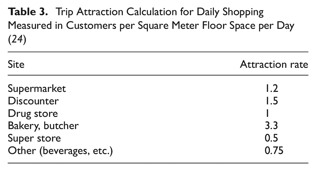
Table 3 presents the calculation method for the example of daily shopping as the trip purpose. It includes the relevant sites and the respective attraction rates per 24 h. The attractiveness for the other purposes is calculated in the same way.
Trip Attraction Calculation for Daily Shopping Measured in Customers per Square Meter Floor Space per Day ( 24 )
Validation of Results
We successfully applied the methodology described in the previous section to an agent-based travel demand model for the region of Karlsruhe in Germany and to an agent-based travel demand model of the region of Boston, MA. It was thus necessary to ensure the quality of the data. We validated the results of every step with official data, analyses of OSM history data, or with data used in previous models of the region. Because of compliance issues, we only show the result for the travel demand model for the region of Karlsruhe. The model was created as a part of the project “Regiomove” and includes about 2 million inhabitants of the region, looking at their activities across an entire week. The model will be used by the local transit agency for demand forecasting, giving it a practical purpose in testing new technologies.
Official Data
The official infrastructure register of the regional planning authority (Regionalverband Mittlerer Oberrhein) was available as an extrinsic comparative dataset for a sub-area of the model. It contains spatial information of manually collected POI data. For the comparison, the 489 travel analysis zones of the model for the sub-area are used. The presence of POIs in the OSM data is then compared with the POIs in the register data for each zone. For grocery stores, 13.1% of the zones are listed in both sources. In 2.5% of the cases, only the OSM dataset has grocery stores recorded and in 2.0% only the infrastructure register contains POIs for the zones. The remaining 82.4% do not contain grocery stores. Thus, both datasets match for 95.5% of the zones. The same comparison was also made for sports facilities (including “leisure = sports_centre,”“stadium,”“pitch building = sport_centre,”“sport_hall”). For 54.0% of the zones none of the sources list such facilities. For 24.3% of the areas examined both datasets contain sports facilities. In 18.8% of the zones only OSM has corresponding POIs. On the other hand, the infrastructure register is the only source for POIs in 2.9% of zones. This is partly a result of a broader definition of the term sports facilities by OSM. This broader definition makes it essential to take into account the dimensions and types of facilities needed to model realistic attractiveness for the POIs in OSM. Random checks reveal the lack of timeliness of the infrastructure register or the inaccurate tagging in OSM, for example, a source of error could be an area marked only as “landuse = retail” rather than “grocery store.”
In a further step, the differences between the shop areas in square meters per zone are compared and the largest deviations examined. The OSM data are more up-to-date in most cases, so stores that are already closed are still included in the official data but not in OSM. In four zones, supermarkets were not included or the calculated areas were smaller by a factor of more than two in OSM. The smaller areas in OSM are mainly caused by multilevel buildings without level information being tagged. However, if all necessary information is included in OSM, the area can be calculated much more precisely than with official data.
OSM History Data
As mentioned in the Open Street Map section, OSM allows for intrinsic evaluation of data quality. One method is to analyze the number of elements over time using historical OSM data. Since OSM data are updated constantly, snapshots of OSM data are made at certain time intervals to ensure that someone can work with the same data status at any time in the future. If the number of elements for a special filter is still growing, one can assume that the process of mapping the elements in OSM is ongoing. When the number of elements remains more or less the same over a period of time, one can assume that this process is completed. Therefore, the measure assessed is the degree of completeness of the map. We are aware that the mapping will never be complete because of the dynamics of land development. But we use the term completeness anyway to indicate that all current elements are mapped, except elements underlying the dynamic.
Figure 2 shows the number of POIs over time from 2009 to 2020 by type of representation for two activity types of the travel demand model: shopping and private business. Whereas the number of shopping POIs has remained more or less the same since 2018, the number of private business POIs is still increasing. Further, the number of polygons remained constant over the past 6 years for both activity types. Assuming that larger and more important POIs are mapped as polygons, we conclude that only smaller and less important POIs are still being added. However, we conclude that in the status-quo of OSM data, POIs for private businesses are not fully included yet and those POIs, therefore, have to be reviewed manually, even if the most important POIs seem to be mapped. Further, we suggest applying this evaluation method on the POIs of every activity type.
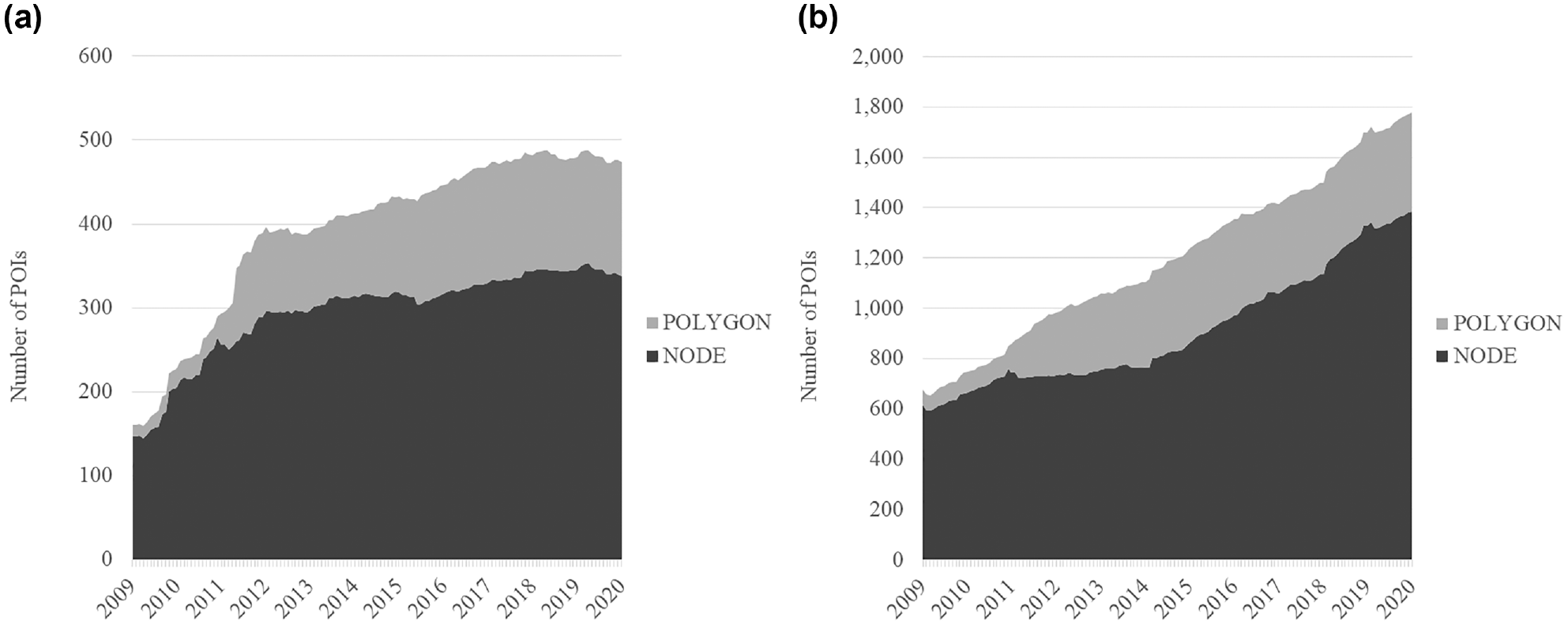
The number of points of interest (POIs) in OpenStreetMap for two different activity types in the region of Karlsruhe since 2009: (a) shopping; and (b) private business.
Travel Demand Model
To evaluate the quality of resulting attractiveness for the travel demand model, it is important to consider the relative differences, as described in the section, Application of Data. We, therefore, compare: the relative differences of attractiveness prepared in this study; the attractiveness of an existing travel demand model for the same region; and the visitor counting data of selected destinations (Table 4). The attractiveness of the existing model is comparable in activity types and represents the state as of 2008. As it is used in planning practice, we compare attractiveness although no clear information is given on its calculation and it represents an older time period. Visitor countings consist of a collection of newspaper articles, statistics, and announcements of respective POIs. We only compare within a category (e.g., water parks) even though all categories are calculated in visitors per 24 h. Relative differences are given in relation to the medium POI in relation to visitor counting.
Model Attractiveness of the OpenStreetMap Founded Model (Model 2020), the Existing Model (Model 2008), and Visitors of the Sights
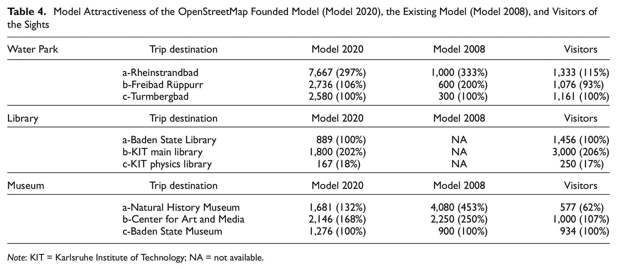
Note: KIT = Karlsruhe Institute of Technology; NA = not available.
Looking at the relative differences of water parks, water parks “b” and “c” are within the same range in relation to visitor counting, even though they differ in absolute terms. Water park “a” represents the largest water park and therefore gets the biggest attractiveness, which can also be seen in the visitor counting. In relation to this, it does not fulfill its expectations as it is only a larger lawn which creates the difference in attractiveness. Further its location is less integrated into the city which compensates for the relative difference by resulting in fewer trip ends in the model. The model data of the existing model perform slightly worse than the modeled OSM attractiveness. The results for libraries best capture the reality. Relative differences only vary marginally. The libraries considered are located in the city center where their accessibility will have only a small influence on the resulting trip ends in the travel demand model, which explain the values obtained. This is only possible as all compared libraries contain information about the number of floors of the building. The modeled results of selected museums reveal a broader variation of attractiveness depending not only on the floor space of the buildings but also on the topic of the exhibition. Further, the data suggest a non-linear interrelation of floor space and visitors. Still, variation is lower when looking at the OSM attractiveness.
In summary, modeled attractiveness and visitors statistics are only comparable to a certain extent. The former misses the influence of accessibility and the nearby population. Further, the approach misses information on special characteristics of POI leading to a higher variation in results. This is in line with the literature; de Gruyter ( 27 ) discovered an “extensive range of site contextual factors.” Nevertheless, the attractiveness generated copes well with those challenges and enables the integration of further site specific characteristics if more detailed attraction data are available. The calibration of input data is not common. However, as these input data are generated by our methodology, it would be appropriate to consider possible adjustments in the main calibration process.
Conclusion and Future Work
We developed an approach for calculating the attractiveness of traffic analysis zones for various activity types. The process is the same for all activity types and can, therefore, be transferred to other activity types. The only difference is the mapping of tags to activity types and the attraction rate per activity type and site category. Because of its nature, the methodology can also be used on single POIs, and this is planned in future research.
However, the data must be of a certain quality to calculate reasonable measures of attractiveness. This can be an issue with, for example, multilevel buildings, as the number of floors is often missing. We, therefore, propose combining data from OSM with other data such as building models to complete the missing number of floors and other information. Another issue that arises with the available information per activity type is that, for different activity types, the number of available POIs varies considerably. While for shopping the amount is quite stable, for private business it is not. Despite these drawbacks, for some activity types, we found that OSM data are more complete and more up-to-date than official data sources. We recommend comparing and evaluating separately the trust in the OSM and official data for each activity type. We further recommend using the historical data as one kind of plausibility check. It quickly provides an impression of the quality of the data in relation to its stability or volatility over time.
As a result of the availability of OSM world wide, this approach can be widened both to other activity types and to other regions. We have applied this approach to build travel demand models in the United States and Europe. One model in Europe is situated in a cross-border region in south-west Germany. It spans districts from multiple countries and multiple states in one of the countries. The spatial transferability of the approach enabled us to build our model on the same database for all districts involved, no matter which country they belong to.
In this study, we applied the methodology manually by using the available tools such as Osmosis, JOSM, and ArcGIS. However, the structured format of OSM data allows further automation of the approach into a single processing chain. An automated process reveals the potential of a much faster estimation of attractiveness. Compared with manually gathered data from various sources, the data fusion can be dropped while the plausibility check can be done in the same manner for all regions of interest. As well as faster generation of models, automation further allows a much faster update of existing models. The same methodology can be applied various times for the same region using a newer OSM dataset. It even enables the user to build attractiveness measures for various years or months allowing the results to be analyzed along with the sensitivity of the model in the context of data changes over time.
As the data can be gathered automatically for various different regions, the effects of data quality on the results of the model can be analyzed, for example, using data of a region with poor quality data compared with a region with high quality data. In such a scenario one could compare the different structural effects of poor and high data quality. Thereafter, a set of metrics could be developed to give a quick impression of the transport-related quality of data in the region comparable to the data viewer Ohsome for historic data. Such metrics could also include an automatic comparison to other open data sources.
Besides the technical improvements following such an automated approach, processing data in an automated fashion and creating value out of it might raise legal concerns. Before using automatically processed OSM data in a travel demand model, one should first consider all restrictions from licenses on the data. As OSM is distributed with an open data license using the data commercially and possibly enriching the data with other data sources might conflict with the OSM license, restrict the usage of the data to academic purposes, or enforce publication of the resulting model.
POIs of OSM provide great potential for calculating measures of attractiveness for travel demand models. Aside from the actuality of the data, their openness makes travel demand models more transparent and should thus be elaborated further in the future. We now have the methodology to calculate measures of attractiveness for any spatial aggregation, even for single POIs.
Footnotes
Author Contributions
The authors confirm contribution to the paper as follows: study conception and design: Christian Klinkhardt, Tim Wörle, Lars Briem, Michael Heilig, Martin Kagerbauer, Peter Vortisch; data collection and application: Christian Klinkhardt, Tim Wörle; analysis and interpretation of results: Christian Klinkhardt, Tim Wörle, Lars Briem, Michael Heilig; draft manuscript preparation: Lars Briem. All authors reviewed the results and approved the final version of the manuscript.
Declaration of Conflicting Interests
The author(s) declared no potential conflicts of interest with respect to the research, authorship, and/or publication of this article.
Funding
The author(s) received no financial support for the research, authorship, and/or publication of this article.