
Abstract
State departments of transportation (DOTs) typically perform annual pavement condition inspections, which serve as an important input into pavement management systems (PMS) software. Road surface defects (cracking, rutting, smoothness, etc.) are analyzed by PMS software to model the deterioration of pavements and to make budget and performance-based recommendations about which roads to maintain and how and when to maintain them. Increasingly at the state DOT level, these data are captured using high-speed 3D lasers (laser triangulation systems) that acquire the 3D shape of the road surface to evaluate its condition. Traditionally the capture of road elevation data relied entirely on the use of survey crews. Although accuracy can be quite high, the process of capturing elevations can require a lot of manpower, is time-consuming, requires lane closures, and results in a relatively small number of points per kilometer of road with which to perform all of the tasks from early project planning through construction. This paper explores an alternate approach that leverages existing 3D laser technology utilized by DOTs to measure the condition of in-service pavements. Typically, these laser systems capture “relatively referenced” 3D profiles of the roadway to evaluate pavement condition based on surface distortion. However, there is often no connection between these “relative” 3D profiles and real-world locations. This new approach involves the addition of high-accuracy blended global navigation satellite system + inertial navigation system positioning systems, as well as specialized software, to map the absolute position of 3D profiles in real-world coordinates.
Keywords
State departments of transportation (DOTs) typically perform annual pavement condition inspections, which serve as an important input into pavement management systems (PMS) software. Road surface defects (cracking, rutting, smoothness, etc.) are analyzed by PMS software to model the deterioration of pavements and to make budget and performance-based recommendations about which roads to maintain and how and when to maintain them. Increasingly these data are captured using high-speed 3D lasers that acquire the 3D shape of the road surface to evaluate its condition ( 1 – 5 ).
Once it is determined that the road condition has degraded to the point that it needs to be rehabilitated and resurfaced, an elevation survey is required. In fact, road surface elevation data play a critical role throughout the entire process of rehabilitating a road.
Elevation data are used during the cost estimation phase in early project programming when the preliminary design estimate is prepared ( 6 ). During the preliminary design stage, civil engineers often make use of planning tools such as AASHTO’s Trn.sport software to perform volumetric estimations and to generate a “length–width–depth” (LWD) cost for prospective projects ( 7 ). LWD estimates include the volumes of material that must be removed, put in place, and compacted.
Later in the life of the project, during the final design stage, elevation data are used by engineers as an input into 3D computer assisted design (CAD) road design software to create the preliminary and final project designs ( 7 ).
During the construction phase, elevation data are used as an input to laser tracking total stations to control 3D pavers and millers ( 8 – 10 ). At the conclusion of construction, elevation data play a role in evaluating whether the new road surface conforms to the geometric design and whether it meets smoothness requirements.
Traditionally the capture of road elevation data relied entirely on the use of survey crews. Although accuracy can be quite high, the process of capturing elevations can require a lot of manpower, is time-consuming, requires lane closures, and results in a relatively small number of points per kilometer of road with which to perform all of the tasks from early project planning through construction.
This paper explores an alternate approach that leverages existing 3D laser triangulation technology utilized by DOTs to measure the condition of in-service pavements. Typically, these laser systems capture “relatively referenced” 3D profiles of the roadway to evaluate pavement condition based on surface distortion. However, there is often no connection between these “relative” 3D profiles and real-world locations.
This new approach involves the addition of a high-accuracy global navigation satellite system (GNSS) integrated with an inertial navigation system (INS), as well as specialized software, to map the absolute position of 3D profiles in real-world coordinates. The result is effectively a fully surveyed pavement surface, at similar accuracy to a traditional survey, captured at speeds up to 100 km/h, without the need for lane closures or to make a separate data collection run in addition to the existing annual pavement condition survey. Figure 1 outlines a possible usage scenario based on this approach, supporting the guidance of laser-controlled milling and paving machines.
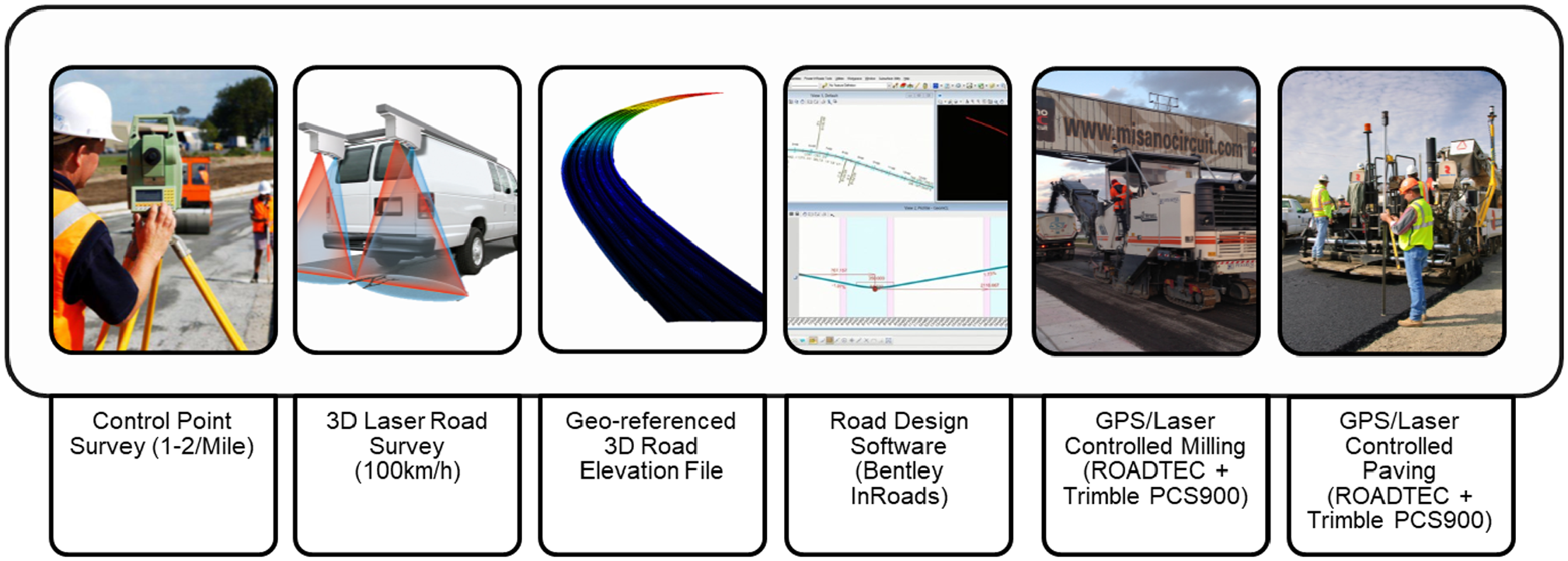
3D pavement elevation modeling workflow.
System Configuration
The 3D laser triangulation technology employed for this project utilizes two 3D laser profilers to acquire 4,000-point 3D transverse profiles of a road lane. The high scanning rate of the system permits the acquisition of transverse profiles at 1 mm intervals at speeds of up to 100 km/h. Thus, the effective points per second (PPS) of the system is 112,000,000 (28,000 Hz × 4,000 points per scan), which is approximately 100 times that of typical mobile LiDAR sensors, which produce upwards of 1,000,000 PPS.
Each sensor head contains an inertial measurement unit (IMU) that is used to monitor the orientation of each sensor during data collection and in the reporting of road roughness as well as roadway geometry.
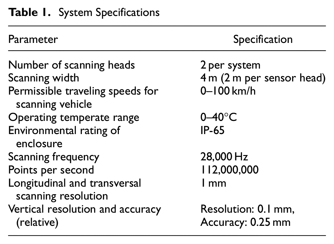
Technical specifications related to the 3D laser triangulation system are presented in Table 1.
System Specifications
These pavement inspection sensors are typically mounted at the rear of the inspection vehicle, perpendicular to the pavement, with each sensor capturing one-half of the driven lane (Figure 2).
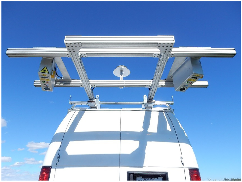
Photograph of the 3D laser profilers and global positioning system (GPS) antenna on the survey vehicle.
For a standard pavement condition application, the 3D point clouds generated by this system are 4 × 10 m in size and are georeferenced to an accuracy of approximately 60 to 100 cm. These point clouds are processed by automated algorithms to extract road surface distresses such as cracks, ruts, pot holes, aggregate loss, and surface texture. Reported pavement defects therefore have a real-world positional accuracy of approximately 1 m.
To utilize these 3D point clouds for a road survey application (in addition to their primary application) the accuracy must be significantly increased and the georeferencing must extend to individual points in the cloud as opposed to 4 × 10 m scans. Additionally, the scans must be corrected for roadway geometry, vehicle and suspension motion, driver wander, and vibrations. The additional hardware, software, and processing steps required to achieve this objective are discussed at length in the following sections.
Additional Hardware and Software Required for Surveying
A high-accuracy blended INS consisting of a GNSS, a wheel encoder (a DMI for measuring linear distance), and an IMU (in addition to the embedded IMU in each sensor head), must be added along with software to map the calculated GPS coordinates to individual points (Figure 3).
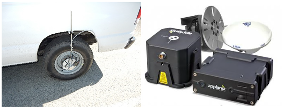
Photograph of wheel encoder and inertial navigation system (INS) including global navigation satellite system (GNSS) receiver, antenna, and inertial measurement unit (IMU).
The blended INS combines GNSS positional data and dead-reckoning data (via the system IMU) to provide the most accurate position possible as an input to the 3D sensors. GNSS and IMU technology are complementary in that dead-reckoning can be used by the INS to continue to provide a position when the GPS signal is lost, with the understanding that the accuracy of the solution will degrade over time (a phenomenon known as “drift”). However, when the GPS signal is regained, the INS can automatically correct the positional solution based on the now known position.
System Calibration
System calibration is required to map the different physical locations and coordinate systems of the 3D laser surveying system’s components (GNSS, IMU, Laser Sensors, and DMI) on the survey vehicle into a single final reference system (GPS). The purpose of the calibration is to establish a digital model of the position of 3D sensors on the vehicle versus the position of the other elements (GNSS, IMU, DMI).
The calibration process consists of four steps:
Physical measures of the distance between each system component (the “lever arms”),
Scanning of a calibration object,
“Stop-and-go” data collection runs, and
Calibration loops.
Physical Measures of the Different Lever Arms Between Each System Sensors
During this step, the physical distances, the “lever arms,” between system components are measured and recorded (Figure 4).
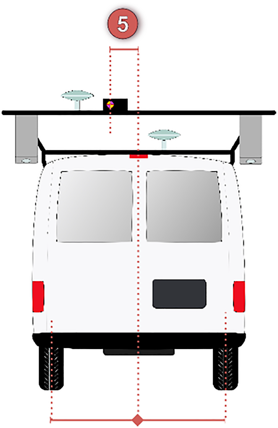
Measuring “lever arms.”
Sensor-to-Sensor Calibration
During this step a precisely dimensioned object is placed on the road surface and the inspection vehicle is driven over the top of it such that the laser scanners capture a scan of it (Figure 5). This step is used to solve the ambiguity between the left and right sensors. The overlap zone between the sensors over the reference object will be used as a reference surface and adjustments will be made in the processing software to account for differences in each sensor’s orientation and mounting position. The end result of this step will be to produce a single combined point cloud from the two sensors that perfectly reproduces the shape of the calibration object.
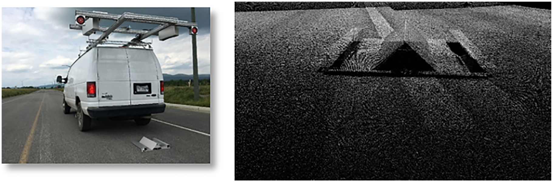
Scan of the calibration object.
“Stop-and-Go” Calibration
The stop-and-go calibration measures acceleration in three axes (X, Y, and Z) using IMUs embedded in each sensor, while the vehicle is both stationary (the “stop” part of the calibration) as well as while it is accelerating (the “go” part of the calibration). This information is used to determine the orientation of the sensors relative to gravitational force.
Dynamic Calibration
This final step in the calibration is used to compensate for the natural degradation of positional accuracy because of IMU drift over time. This compensation is performed for the IMU contained in the integrated GNSS+INS system.
Data captured is used to fine-tune the biases of the gyroscope and accelerometers that are contained in the IMU so as to ensure a perfect match of the scans from the two sensors when combined.
This step requires three special calibration runs, “loops” (Figure 6), “back-through loops” (Figure 7), and “right-angle loops” (Figure 8), to be performed while driving across the calibration object. Loop runs are used to eliminate offsets in pitch measurements that, when uncorrected, result in repeat runs producing spiral patterns rather than properly overlaid loops.
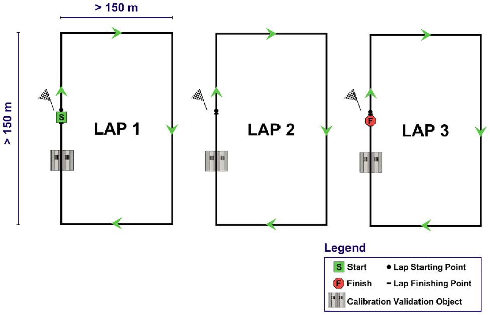
Calibration “loop” runs.
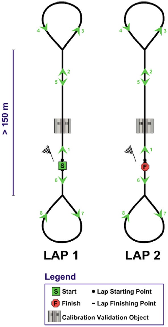
Calibration “back-through loop” runs.
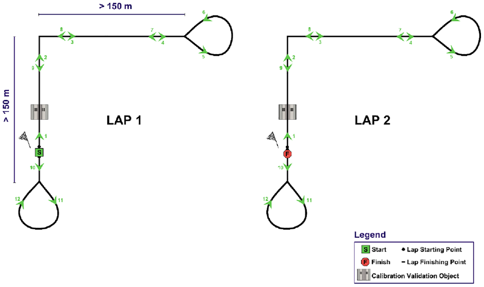
Calibration “right-angle loop” runs.
Back-through loops are used to compensate for roll offsets that, uncorrected, would result in a kind of x pattern for repeat runs as opposed to properly overlaid back-through loops.
Right-angle loops are used to compensate for heading offsets.
Data Capture and Processing
Mapping Vehicle GPS Coordinates to Laser Scan Points
Once 3D scans have been captured in the field and GPS data have been postprocessed (if desired), specialized software is used to translate the GPS positional coordinates of the vehicle to the individual coordinates in the 3D point cloud. There are six steps in this process:
Postprocessing GPS data,
Importing 3D scans in postprocessing software,
Developing the vehicle navigation solution,
Combining multiple adjacent 3D scans into a single surface,
Aligning the 3D surface to ground survey, and
Exporting the 3D roadway model for design.
Postprocessing GPS Data
Although the onboard INS is capable of providing a highly accurate stream of GPS data in real time, the positional solution can be further improved through the use of a GPS base station within 30 to 50 km of the data collection site.
Whereas in the past this task would have required the setup of a dedicated base station for a project, many countries have large networks of established base stations from which the user can obtain data from for free, or for a reasonable fee. For example, in the United States, the National Geodetic Society’s continuously operating reference stations network provides free base station data across the country (Figure 9).
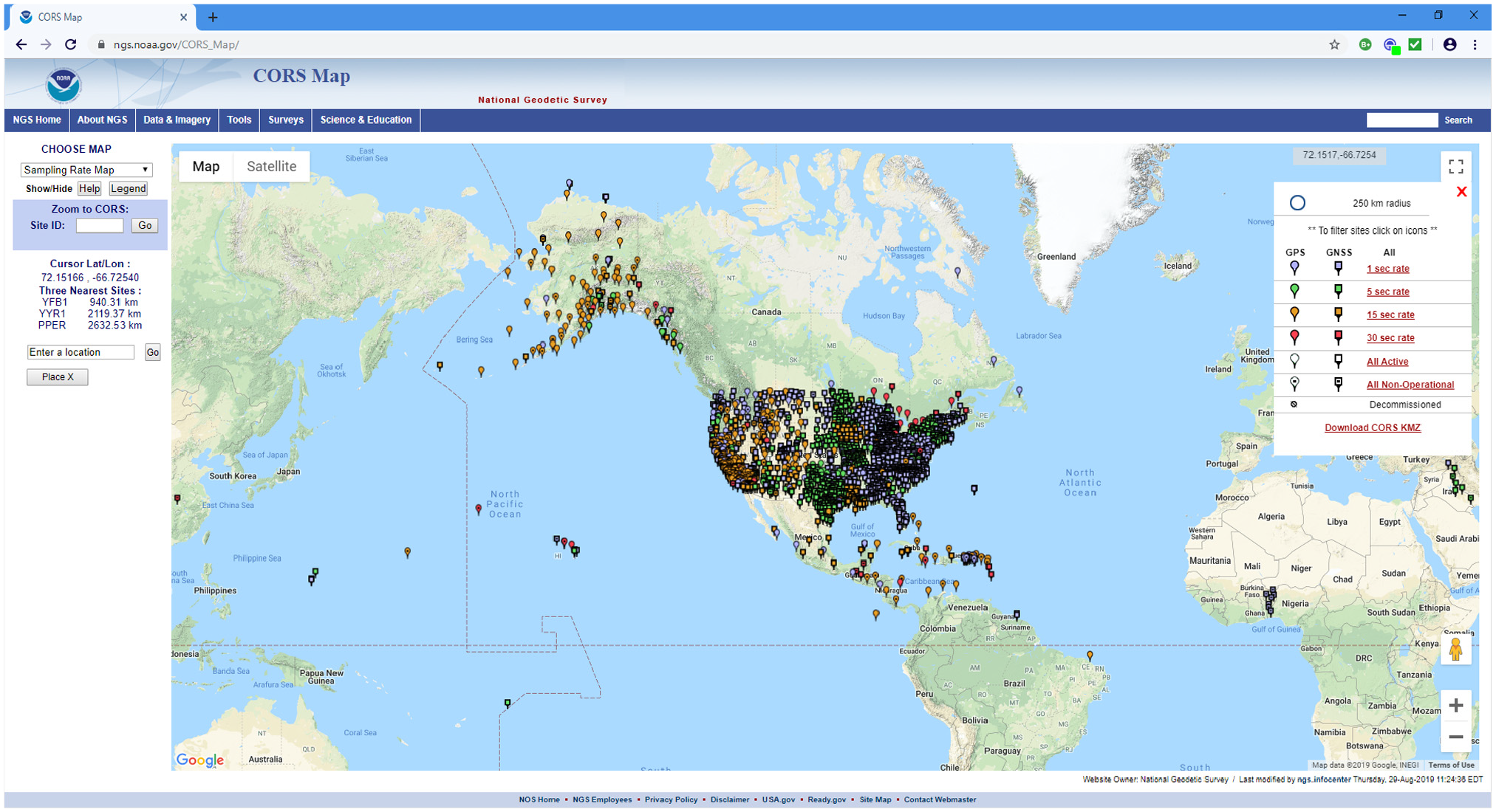
U.S. continuously operating reference stations network.
Postprocessing of the real-time GPS positional solution using base station data can significantly improve the overall accuracy of the final positional solution, which is key for road survey applications. This postprocessing is normally performed using software included with the INS hardware.
If there is no postprocessed data available, it is always possible to produce a 3D surface using the real-time GPS data recorded in the files during the data acquisition, however, accuracy and repeatability will be affected.
Importing 3D Scans into Postprocessing Software
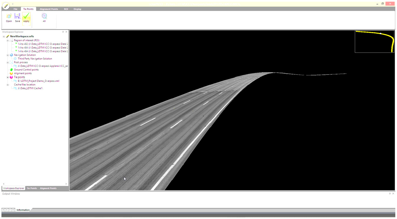
During this step, 3D scans from the field (in FIS format) are imported into a postprocessing software application (Figure 10) along with the real-time or postprocessed GPS track of the inspection vehicle.
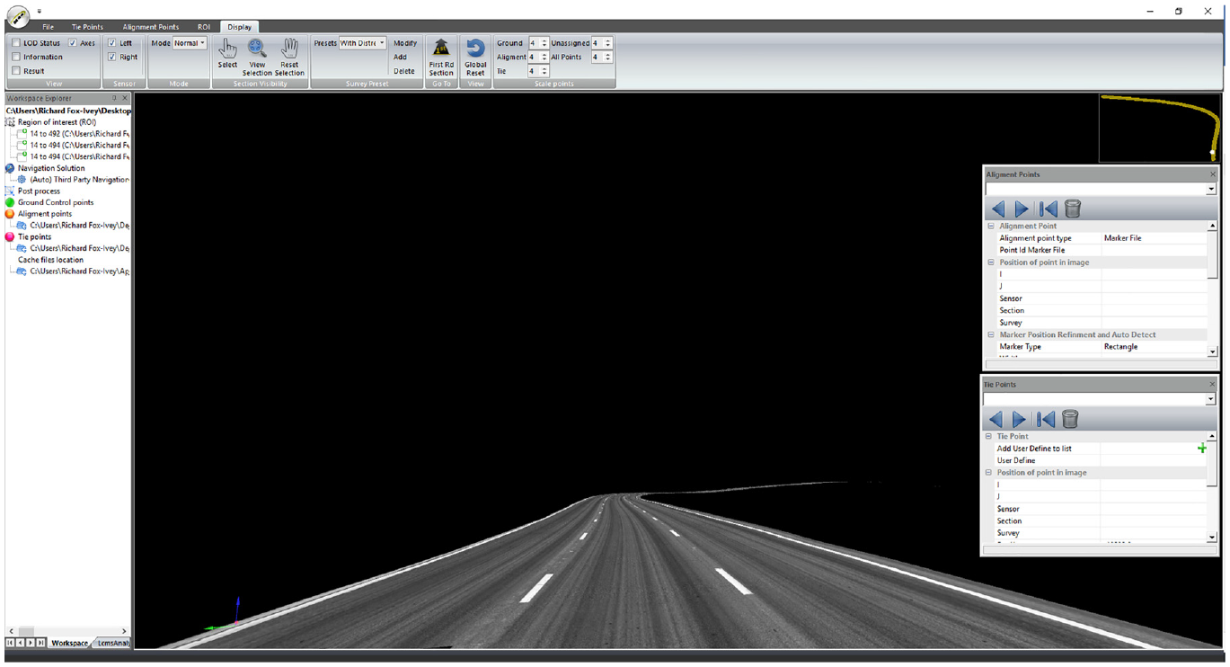
Postprocessing software.
The postprocessing software supports the import of 3D pavement scans, postprocessed GPS data, and ground control coordinates.
Developing the Vehicle Navigation Solution
This step is performed using the postprocessing software and transfers the GPS coordinates of the vehicle, compensated for vehicle motion through the earlier calibration process, to individual 3D points in the laser scan (Figure 11). At this time the accuracy of individual elevation points in the reported surface will be at the same level as the accuracy of the reported vehicle position.
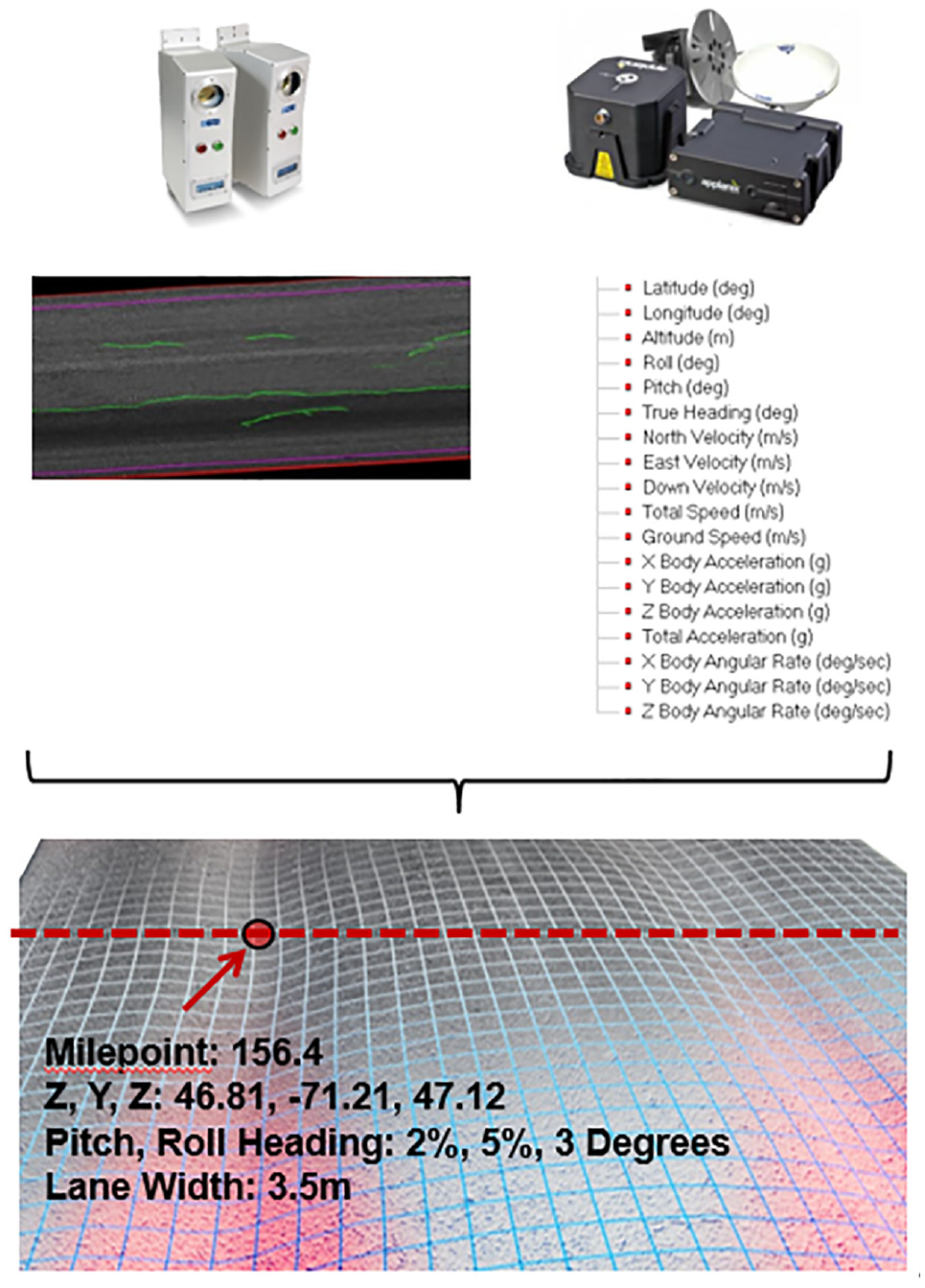
Location system components.
With the application of a high-accuracy INS and the use of postprocessed GPS data, this solution will be in the range of a couple of centimeters accuracy (however it will be significantly enhanced in later steps).
Combining Multiple Adjacent 3D Scans Into a Single Surface
When surveying wide surfaces, such as runways or multilane highways, it will be necessary to make multiple 4-m wide overlapping data collection scans. Following field work, these scans must be merged together to create a single, final, 3D surface to replace a traditional survey.
The process of merging multiple scan passes is referred to as “stitching” and it is an automated process wherein a computer algorithm searches for common features between adjacent overlapping scans (Figure 12). Common features can include anything that is visible on the surface of the pavement (e.g., a pavement marking or an embedded reflector) or something with a unique 3D profile such as a pavement distress (e.g., a crack or a construction joint).
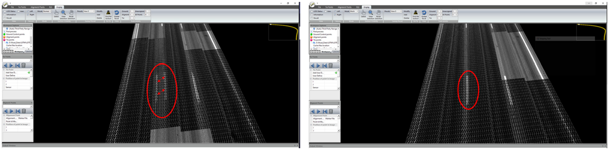
Overlapping 3D scans (left is before stitching, right is post stitching).
Aligning the 3D Surface to Ground Survey
This is an optional step that can be used to further refine the accuracy of the navigation solution by “tying” it to local surveyed control points. This step is recommended for final project surveys that will be used during the construction phase, but could be omitted if the data are being used as a preliminary survey or for a project estimate.
As opposed to a traditional road resurfacing survey that would involve hundreds or thousands of surveyed points per kilometer across the width of the pavement, this process only requires one control point at the very edge of the pavement surface per kilometer.
During this step, circular reference targets are painted at the start of each kilometer on the pavement shoulder, and the latitude, longitude, and elevation of the center of the targets are recorded using a robotic GPS total station (Figure 13). This approach avoids the need for a full lane closure and allows survey staff to work from the safety of the road shoulder.
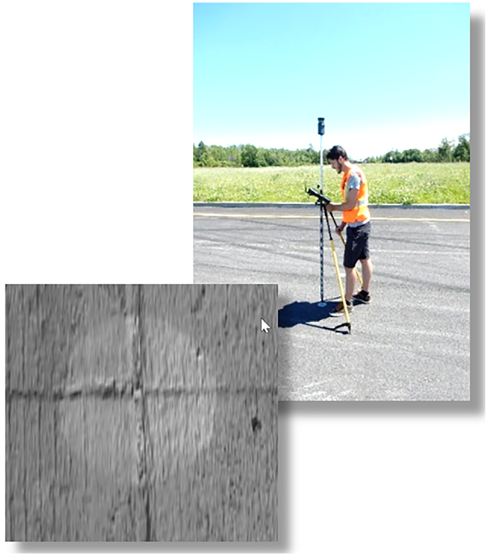
Survey of ground control targets using a global positioning system (GPS) total station.
The latitude, longitude and elevation of the targets can then be entered into the postprocessing software and the 3D surface aligned accordingly (Figure 14).
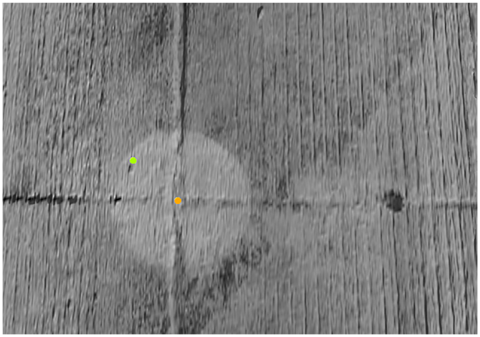
Unaligned target center (green point) and aligned target center (orange point).
Exporting the 3D Pavement Model
Available outputs from the postprocessing software include LAS files containing the ground survey elevations as well as BMPs containing a high-resolution view of the pavement surface. The LAS format is nonproprietary and can be directly imported into numerous 3D CAD road design applications such as AutoCAD®Civil 3D®.
Before exporting survey data, the software allows the user to scale the resolution of the data to reduce point densities as desired; very detailed maps can be generated at resolutions of 100 × 100 mm for example. Points are decimated to fixed resolutions (X, Y) and the vertical (Z) position is filtered to avoid reporting the elevation of loose aggregate, the pavement surface, or of a pavement defect such as a crack.
This final step creates a 1 × 1 mm elevation survey of the pavement surface (Figure 15) with a vertical accuracy matching traditional methods (approximately 3 to 5 mm for elevation).
Final 3 to 5 mm absolute elevation accurate surface (containing three lanes and a bridge deck).
Applications and Benefits of 3D Elevation Data
This enhanced dataset presents a wide range of benefits to the industry. Federal Highway Administration (FHWA) research indicates that 3D laser scanning models can deliver both significant cost savings as well as provide an effective tool for planning and communication between DOTs, contractors, and consultants ( 9 ).
The FHWA’s Techbrief on 3D, 4D, and 5D Engineered Models for Construction reports an average saving of 66% for grade checking, up to 85% savings in reduction of stakes, 3% to 6% savings by volume for improved material yields and 4% to 6% savings in total project costs for projects using 3D models ( 9 ).
Likewise, research published by Michigan DOT indicates significant savings as well:
3D models (indiscriminate of project size) consistently produced bids that were lower than the engineer’s estimate. When bids came in higher than the engineer’s estimate, 3D models produced fewer change orders than 2D plans. MDOT observed a net cost savings of $12.9 million across projects using 3D models … and a net cost overrun of $19.1 million across projects using 2D plans only (
10
)
Savings can be attributed to a variety of sources, including improved earthwork calculations and improved milling and paving operations ( 9 ).
During earthwork, highly accurate 3D elevation models allow for the optimization of material quantities that need to be carried into and out of the construction site.
During resurfacing, automated laser-controlled milling machines can use 3D elevation models to optimize and correct the road’s longitudinal profile dynamically, compared with fixed-depth milling ( 9 ).
During paving, 3D laser-controlled pavers can make use of 3D models to create variable thickness asphalt layers that deliver smoother rides and longer service life owing to reduced axial dynamic loads imparted by heavy vehicles ( 11 , 12 ).
Accuracy Compared to Ground Truth
To establish the real-world positional accuracy of the system (as opposed to the simple relative accuracy of individual points), a pavement elevation reference site was developed that included more than 500 reference points (Figure 16). Reference points were created by painting circular targets at 500 separate locations spread throughout the test site and then surveying the center of each target a total of three times using a robotic total station and a laser level.
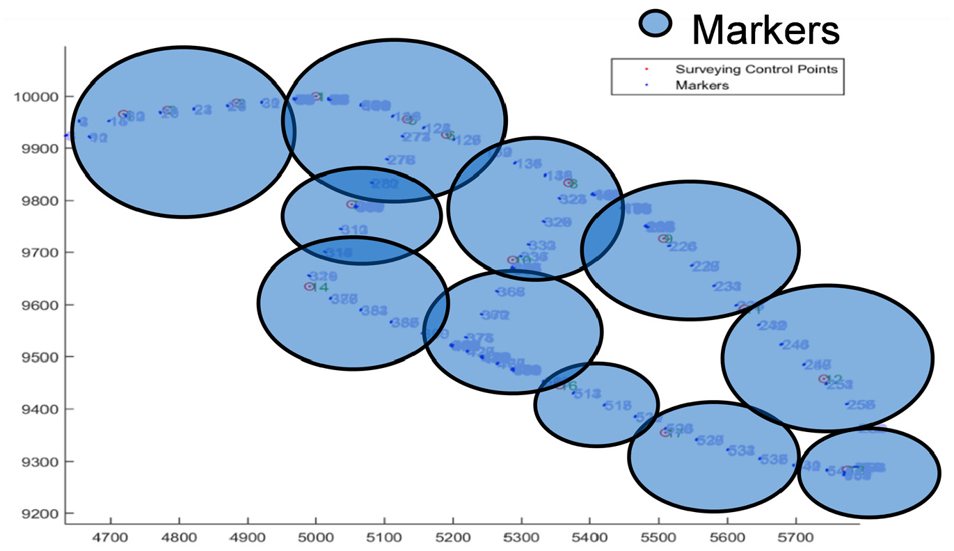
Reference site.
Repeat measurements were used to minimize the error of reported elevations to create a “ground truth” that was as accurate as possible. Using this method, the absolute elevation accuracy of the reference points was determined to be between 2 and 5 mm.
Following the generation of reference points, a survey vehicle equipped with the 3D laser triangulation system (and associated hardware) was driven a total of 12 times through the reference site. Repeat runs were used to ensure a thorough evaluation of the average accuracy of the system compared with ground truth, as well as to determine repeatability.
Accuracy of the system was then evaluated under two different survey-alignment scenarios to explore the tradeoff between resulting surface accuracy and gains in time reductions and safety improvements through the elimination of traditional survey work. Consequently, the focus of the evaluation was to consider alignment scenarios that produced the most accurate 3D surface with the least amount of survey-alignment points.
The first approach utilized an alignment point spacing of 300 m (roughly three per kilometer) and the second approach utilized a spacing of 825 m (roughly one per kilometer). Both scenarios represented a significant reduction in cost, time, and impact to the traveling public when compared with a traditional road survey.
For the 300 m scenario, the average error in elevation measurements across 12 inspection runs for the 3D laser triangulation survey was 2.5 mm for elevation (Z) when compared with ground truth (Figure 17).
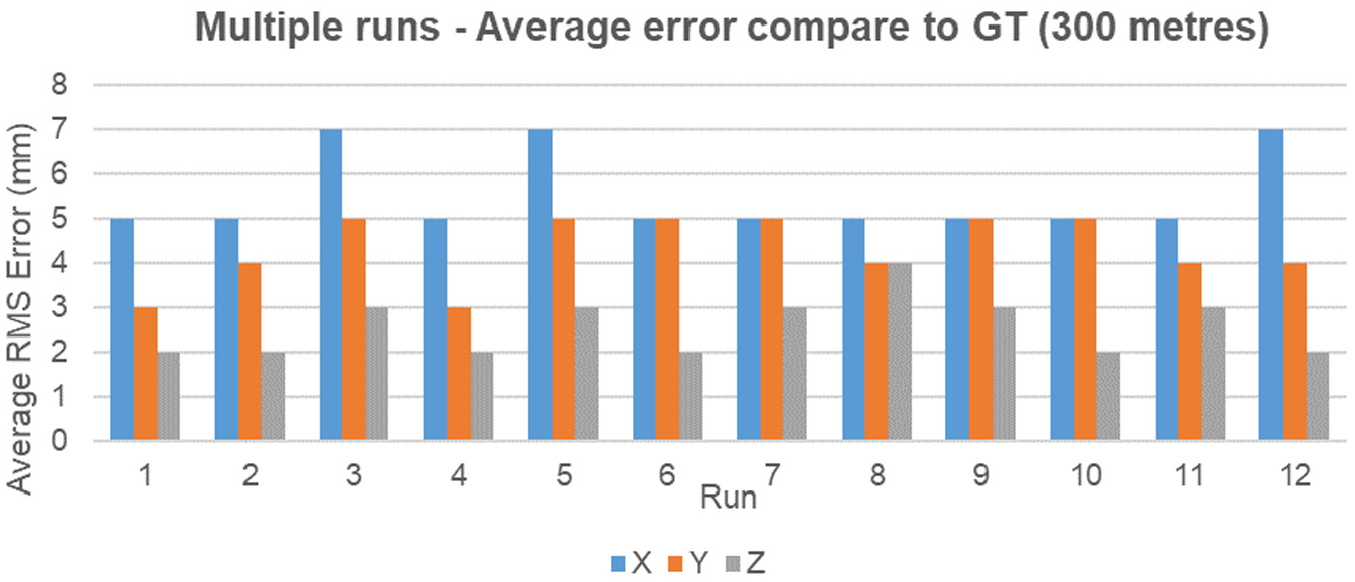
Accuracy of laser triangulation versus ground truth (300 m).
As the accepted accuracy of the ground truth itself was between 2 and 5 mm, a reported accuracy of 2.5 mm for the 3D laser triangulation survey effectively made it identical to a traditional survey. Repeatability of the 3D laser triangulation survey was also excellent with a reported error of just 2 mm for elevation (Z) when comparing the 11 repeat runs to the initial run.
In the 825 m scenario, the number of alignment points used per kilometer of road was reduced from three to just a single point at the edge of the pavement. In this scenario the average error in elevation measurements across the 12 inspection runs was 5 mm for elevation (Z) when compared with ground truth (Figure 18).
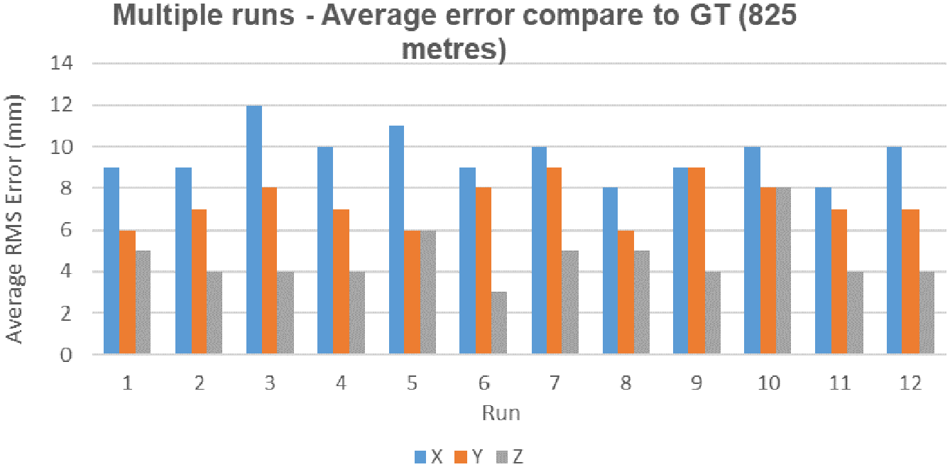
Accuracy of laser triangulation versus ground truth (825 m).
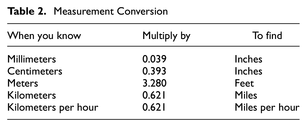
Although the average error of the 825 m alignment scenario was slightly higher, at 5 mm instead of 2.5 mm, it is still within the range of the accepted accuracy of the ground truth itself (2 to 5 mm). Repeatability for the 825 m scenario was also excellent with a reported error of 4 mm for elevation (Z) when comparing the 11 repeat runs to the initial run. Metric to imperial measurement conversions are presented in Table 2.
Measurement Conversion
These results show the clear advantages of this approach over the traditional survey and LiDAR. Traditional surveys typically only provide three elevation points every 20 m longitudinally with which to design surfaces. Likewise, LiDAR-based solutions are often limited in accuracy; compared with traditional survey and the approach described here, LiDAR-based elevations are often only accurate to a few centimeters.
Conclusion
There is an untapped opportunity to enhance and repurpose 3D scans that are being collected solely for the purpose of pavement condition evaluation, such that they could provide the necessary elevation data for project estimates, and the preliminary and final designs of roads slated for resurfacing and reconstruction.
By integrating high-accuracy INS with 3D scans, and the use of specialized software, it is possible to generate 3D surfaces of roads while performing existing annual pavement condition survey inspections. The resulting absolute accuracy of elevation data was in the range of 3 to 5 mm, which is effectively the same accuracy as traditional methods.
This method presents numerous advantages over the traditional approach including:
– Time savings at the project planning stage, as elevation data for the entire road network can be made available without the need to dispatch a survey crew;
– Significant cost savings through the project planning and construction stages, as the number of traditional survey points per mile can be reduced to just a single point;
– Reduced impact on the traveling public by nearly eliminating the need for road closures related to surveys; and
– Increased safety by reducing the exposure of survey staff to traffic.
Footnotes
Author Contributions
The authors confirm contribution to the paper as follows: study conception and design: J. Laurent, B. Petitclerc, R. Fox-Ivey; data collection: B. Petitclerc; analysis and interpretation of results: J. Laurent, B. Petitclerc; draft manuscript preparation: R. Fox-Ivey. All authors reviewed the results and approved the final version of the manuscript.
Declaration of Conflicting Interests
The authors declared no potential conflicts of interest with respect to the research, authorship, and/or publication of this article.
Funding
The authors received no financial support for the research, authorship, and/or publication of this article.