
Abstract
Dhaka, one of the fastest-growing megacities in the world, faces severe traffic congestion leading to a loss of 3.2 million business hours per day. While peak-spreading policies hold the promise to reduce the traffic congestion levels, the absence of comprehensive data sources makes it extremely challenging to develop econometric models of departure time choices for Dhaka. This motivates this paper, which develops advanced discrete choice models of departure time choice of car commuters using secondary data sources and quantifies how level-of-service attributes (e.g., travel time), socio-demographic characteristics (e.g., type of job, income, etc.), and situational constraints (e.g., schedule delay) affect their choices. The trip diary data of commuters making home-to-work and work-to-home trips by personal car/ride-hailing services (957 and 934 respectively) have been used in this regard. Given the discrepancy between the stated travel times and those extracted using the Google Directions API, a sub-model is developed first to derive more reliable estimates of travel time throughout the day. A mixed multinomial logit model and a simple multinomial logit model are developed for outbound and return trip, respectively, to capture the heterogeneity associated with different departure time choice of car commuters. Estimation results indicate that the choices are significantly affected by travel time, schedule delay, and socio-demographic factors. The influence of type of job on preferred departure time (PDT) has been estimated using two different distributions of PDT for office employees and self-employed people (Johnson’s SB distribution and truncated normal respectively). The proposed framework could be useful in other developing countries with similar data issues.
Dhaka, the capital of Bangladesh, is home to more than 15 million people. The population of Dhaka (within the Rajdhani Unnayan Kartripakkha [RAJUK] jurisdiction area, which is the Capital Development Authority of the Government of Bangladesh) is projected to be 26.3 million by the year 2035, predominantly as a result of migration from rural to urban areas ( 1 ). To meet the mobility demand of this rapidly growing population, the number of motorized vehicles in the city, private cars in particular, is increasing at an alarming rate. According to the statistics of the Bangladesh Road Transport Authority, a total of 145,000 private cars, 20,000 trucks, and 14,000 buses and minibuses are currently registered in the Dhaka Metropolitan Area, and their numbers are expected to grow at a rate of 34% annually. This escalating growth of motorized vehicle coupled with the increasing usage of private vehicles is associated with the severe traffic congestion that cripples the city and results in a loss of 3.2 million business hours per day ( 2 ).
The traffic congestion levels in Dhaka are worst during the morning and evening peak hours. According to the World Bank ( 3 ), the average speed on Dhaka’s urban network during peak hours is approximately 8.75 km/h, indicating that the travel time during the peak hours is almost triple the travel time during the off-peak hours. Many of the trips made during these periods are presumed to be mandatory trips by commuters that are often hard to cancel or reschedule. However, different types of commuters are expected to have different levels of flexibility in their start times at their workplaces as well as their commitments at home. It is, therefore, crucial to develop an understanding of the factors affecting the departure time choice decisions made by the commuters and how they vary with the type of their job and socio-demographic characteristics. It is then a matter of identifying the appropriate modeling specifications that can reflect the behavior of decision-makers about departure time choice that can be used to design policies to flatten the peak demand.
Although departure time choice is a crucial determinant in measuring the temporal and spatial distribution of travel demand ( 4 ), it has received less attention than mode or route choice ( 5 , 6 ). For example, previous travel demand models developed that focused on Dhaka city discussed methodological issues in developing the mode choice model ( 7 ) but there has not been similar research done in the context of departure time choice. Key challenges to developing a departure time choice model in the case of Dhaka (as well as many countries in the developing world) include the following:
(1) lack of dependable data sources to calculate the travel time for different origin–destination pairs.
(2) different opening and closing times of different types of institutions making it harder to infer the preferred departure time choice.
In the context of developed countries, several modeling approaches have been used to model departure time choice. Bhat and Steed ( 8 ) developed a continuous time model for urban shopping trips. In parallel, many studies have used discrete choice models to investigate departure time choice by dividing the continuous departure time variable into a finite set of discrete intervals. For example, Small ( 9 ), McCafferty and Hall ( 10 ), Hendrickson and Plank ( 5 ), and Holyoak ( 11 ) used simple multinomial logit (MNL) structures to model departure time choices of commuters. MNL models have also been used to model time of day choice in the context of trips made during weekends and holidays ( 12 , 13 ). In addition to the single facet model, Bhat ( 14 ) used a joint MNL and ordered generalized extreme value formulation for integrated models of mode and departure time choices. That study, however, focused only on non-commute trips. De Jong et al. ( 15 ) and Hess et al. ( 16 ) used mixed MNL (MMNL) models to capture the influences of unobserved factors in the time of day switching in the context of mode and departure time choices. However, all these studies and their applications focus on countries in North America and Europe which, compared with developing countries like Bangladesh, have very different socio-economic composition (e.g., income and age distribution, gender roles, household size and family structure, etc.), work culture (e.g., inflexible working hours, recording of arrival time at workplace, etc.), state of technological advancement (e.g., reliable internet access and uninterrupted power supply to work from home) and transport landscape (e.g., car ownership levels, public transport accessibility, paratransit, etc.). All these lead to significant differences in activity and travel behavior ( 7 , 17 , 18 ) and affect the transferability of the models ( 17 – 19 ). Further, modeling frameworks formulated for the developed countries are very often not directly applicable in the context of developing countries where detailed socio-demographic information and fine-scale spatial and temporal data are not available ( 7 ).
Very few studies have discussed the methodological issues and data challenges of modeling departure time choice in the context of developing countries ( 20 , 21 ). Anwar ( 20 ) proposed a departure time choice model in the context of Dhaka using primary data with a pre-defined classification of timeslots within a narrow range (7:30–8:50). The collected data was used to develop ordered logit models of departure time choice. However, the study focused only on officials who had office hours from 09:00 to 17:00, ignoring the rest of the working population. Further, the travel times used in calibrating the model lacked adequate temporal and spatial granularity.
This motivates this research, which develops advanced discrete choice models of departure time choice of car commuters using secondary data sources. It proposes approaches to account for the data limitations and quantifies how the level-of-service attributes (e.g., travel time), socio-demographic characteristics (e.g., type of job, income etc.), and situational constraints (e.g., schedule delay, activity duration) affect the departure time choices of different types of commuters. Trip diary data of commuters making home-to-work and work-to-home trips by personal car/ride-hailing services (957 and 934, respectively) have been used in this regard. It may be noted that although stated preference data have been used in some of the departure choice modeling studies ( 6 , 15 , 16 , 21 , 22 ), it is prone to hypothetical bias and behavioral incongruence ( 23 ) and therefore revealed preference (RP) data has been deemed to be the better option. To the best of the authors’ knowledge, this is the first study that highlights the key challenges and methodological issues to model departure time choice using RP data from developing countries and proposes ways to address these issues.
The rest of the paper is organized as follows: the next section describes the data sources used in this study. The modeling issues are presented next followed by the description of the model structure and the estimation results. The findings are summarized at the end of the paper along with directions for future research.
Data
This study used travel diary survey data conducted across the Dhaka Metropolitan Region (RAJUK area) by TYPSA (https://www.typsa.com/en/) as part of the Dhaka Subway Project. The data was collected from Monday to Saturday between February 28, 2019 and May 4, 2019. It should be noted that Friday is the general weekly holiday in Bangladesh. Educational institutes and some offices are closed on Friday and Saturday. A total of 35,000 households were surveyed in the RAJUK area. A stratified sampling procedure with proportional allocation was applied to determine the number of households to be surveyed in each sub-divided area. About 25,000 households were surveyed in the Dhaka City Corporation area, with the remaining 10,000 household interviews conducted in the rest of the RAJUK area. During the surveys, each household member was asked about trips made during the previous working day (from Sunday to Thursday). The questionnaire survey was divided into two parts: the first part focused on general household information (e.g., age, gender, education, occupation, income, car ownership) and the second part focused on trip-related information (e.g., departure time, travel mode, travel time) for each household member who had made at least one trip on the previous working day. Very short trips (less than 10 min of walking distance) and trips made by children (under 6 years) were not recorded. The survey was well planned to avoid trips made on Fridays, Saturdays, public holidays, hartal (strike days), election days, major events (like Ijtema), and during Ramadan. From the full dataset, only commuting trips by car-based modes (private car and ride-hailing services like Uber/Pathao car) have been considered for this study. Before conducting the survey in each zone, the survey correspondents had communicated with local representatives including the ward commissioners to gain approval of, and assistance for, the surveys. This survey yielded a total of 957 unique home-to-work trips and 934 unique work-to-home trips. There is an imbalance in the number of home-to-work and work-to-home commute trips by car/ride-hailing services as some travelers had used public transport and non-motorized modes in one of the legs of the trip. Commuting trips with origins outside Dhaka have not been considered. The socio-demographic characteristics of the commuters are summarized in Table 1.
Summary of Socio-Demographic Characteristics of the Commuters in the Sample
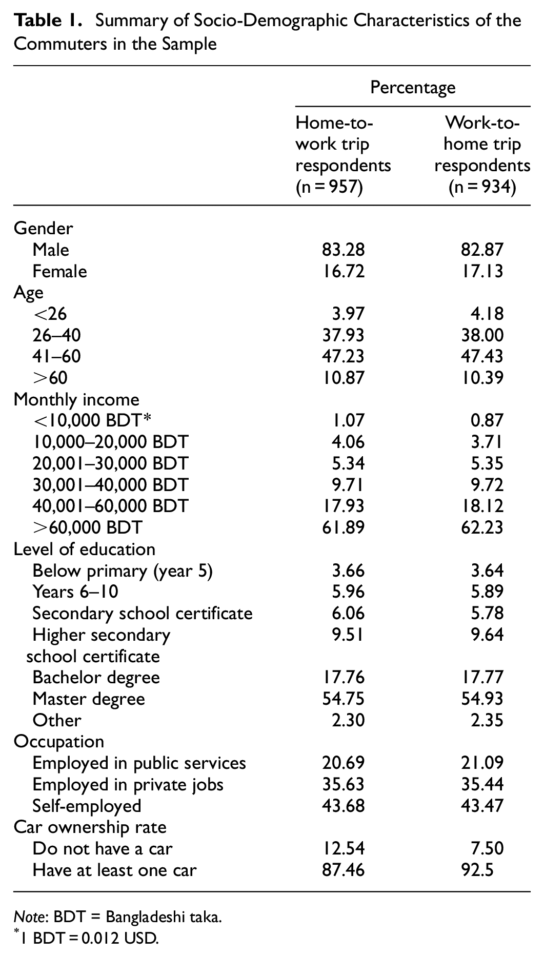
Note: BDT = Bangladeshi taka.
1 BDT = 0.012 USD.
It may be noted that, although the original sample was representative of the population of Dhaka city, the sample used in the departure time choice models of this paper is expected to be biased toward high-income and educated segments of the population as it focuses only on car users (who have higher affordability than the others).
Modeling Issues
Choice Set Specification
The number and length (i.e., duration) of alternative time periods play an important role in the computation, interpretation, and transferability of the departure time choice models ( 24 ). In a usual specification, a separate alternative specific constant (ASC) is recommended for each possible combination of home-to-work (outbound) and work-to-home (inbound) time period to capture the unexplained time preference of travelers. However, this can lead to a compounding problem of higher computational cost and complex parameter identification. For example, using 1 h time periods (N = 24) would lead to a requirement for 300 constants (following the rule N(N+1)/2), of which 299 (N(N+1)/2–1) can be estimated ( 16 ). To reduce this computational cost, a separate set of alternatives for the outbound (home-to-work) and return (work-to-home) trip is used. The choice set for the outbound (home-to-work) trips is assumed to range between 06:00 and 18:00. Between 06:00 and 12:00, 1 h intervals are used (since the majority of the trips are likely to be made before 12:00) and 2 h intervals are used for the rest. The choice set for the return (work-to-home) trips is assumed to range between 10:00 and 24:00. Between 16:00 and 20:00, 1 h intervals are used (since the majority of the trips are likely to be made before 20:00) and 2 h intervals are used for the rest. In the time choice model, the off-peak hours (6:00–7:00, 10:00–12:00) are considered as base alternatives.
Calculation of Travel Time
Departure time choice models require the calculation of travel times between origins and destinations for the chosen and unchosen time periods. In many cities, software such as Google Maps and Open Street Maps provide reliable travel times for each alternative time period with adequate spatial and temporal granularity. Examples include departure time choice models developed in the context of the U.S.A. ( 4 , 23 ) where Google Maps Distance Matrix API/Direction API has been used for deriving travel times during different time periods for different origin–destination pairs. Since Google Maps uses historical data to predict future traffic, it is considered that future traffic conditions based on Google Maps are more stable and represent better trends in traffic than real-time information. However, in the context of a developing country, it is more difficult to infer travel time accurately from Google Maps. For example, in Dhaka, both motorized and non-motorized vehicles share a common right-of-way, making travel times very sensitive to the proportion of different types of vehicles. Further, in Dhaka, traffic intersections are manually operated by traffic police which also makes it harder to infer travel times reliably between a specific origin–destination pair. Moreover, there are multiple types of public transport and paratransit services (e.g., human hauler, “tempo,” etc.), which tend to allow passengers to board, alight, or both, at almost any place. These also make it almost impossible to predict travel times reliably across the network. Finally, though Google Maps can show the shortest path in Dhaka, the use of navigation technology is not widespread among car users. Most of the cars are chauffeur-driven, and the chauffeurs use their intuition to select the route to travel instead of choosing the quickest or shortest path that would have been recommended by a navigation device. For these reasons, instead of providing a single predicted travel time between an origin–destination pair, Google Maps Direction API provides three different travel time suggestions: best guess, pessimistic and optimistic. The best guess model returns the trip duration in traffic using both historical traffic conditions and live traffic. Live traffic becomes more important the closer the departure time is to the present moment. The pessimistic model returns the trip duration in traffic that usually should be longer than the actual travel time on most days, though occasional days with particularly bad traffic conditions may exceed this value. The optimistic model returns the trip duration in traffic, that usually should be shorter than the actual travel time on most days, however, occasional days often with good traffic conditions could be faster than this value. Comparison of the stated travel time (only available for the chosen time of travel) and the three different predicted travel times showed variations in fit depending on the time of the day and origin–destination pair. This prompted the authors to estimate a sub-model to establish a relationship between the stated travel time and the best guess, pessimistic, and optimistic travel times.
The proposed relationship between the stated travel time and predicted travel time using models from the Direction API can be expressed as follows:
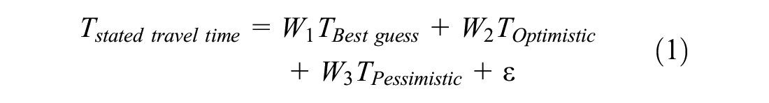
where

were n is the number of alternative time periods (n = 7 for home-to-work and n = 5 for work-to-home trip) and j refers to the number of models (j = 3) considered for travel time prediction. Weights calculated from different Google Maps models are presented in Tables 2 and 3.
Calculated Weights of Different Models Used for Travel Time Calculation (Home-to-Work Trip)
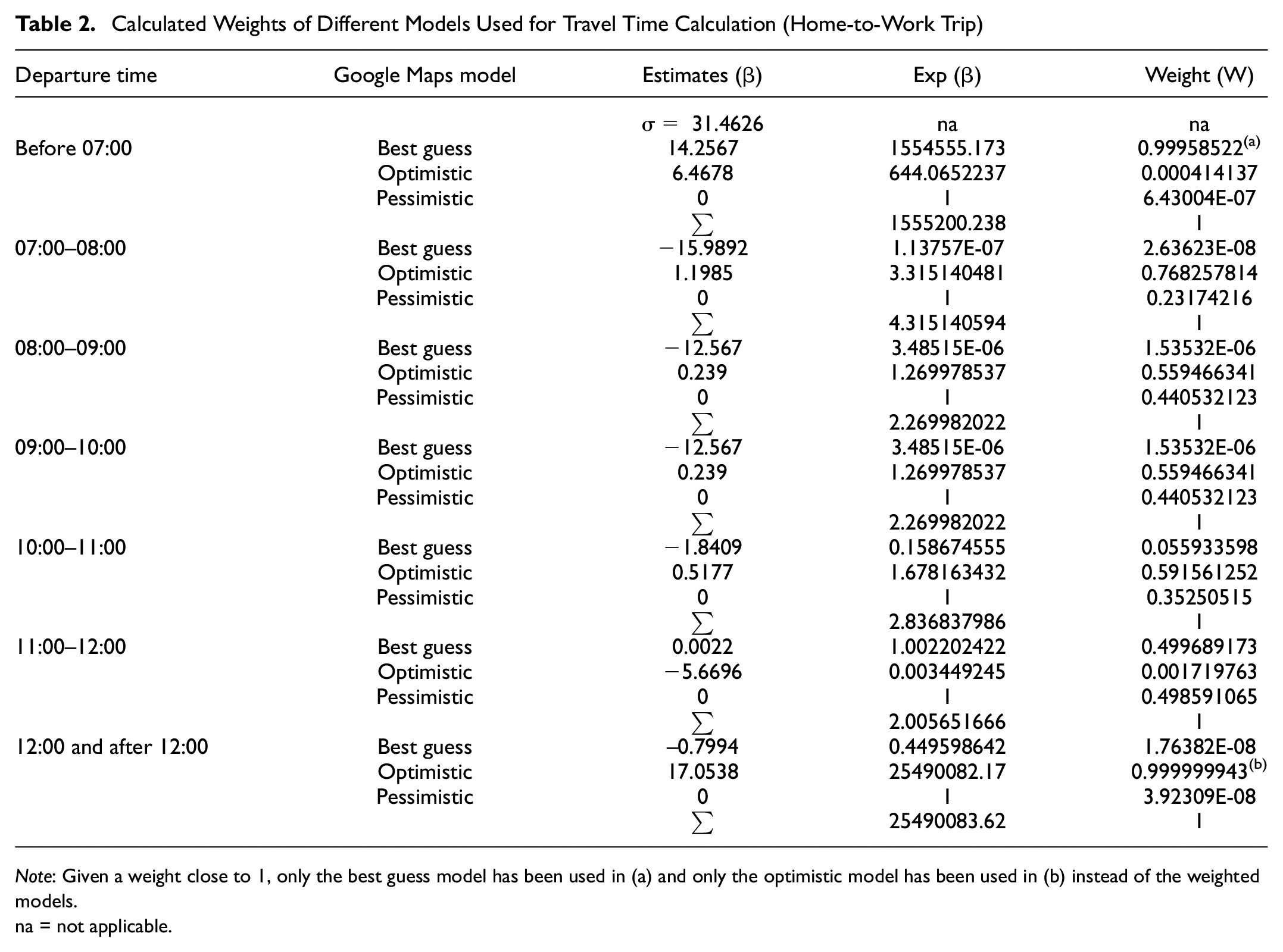
Note: Given a weight close to 1, only the best guess model has been used in (a) and only the optimistic model has been used in (b) instead of the weighted models.
na = not applicable.
Calculated Weights of Different Models Used for Travel Time Calculation (Work-to-Home Trip)
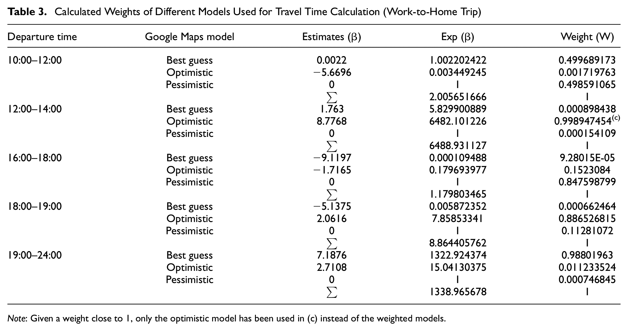
Note: Given a weight close to 1, only the optimistic model has been used in (c) instead of the weighted models.
Further, the fit of the results has been tested by comparing the measured travel times (calculated using the estimated weights) with the stated travel times for each origin–destination pair (Figure 1). The correlation coefficients (0.65 and 0.6 for home-to-work and work-to-home trips, respectively) signify the substantial positive association between the estimated and measured travel times.
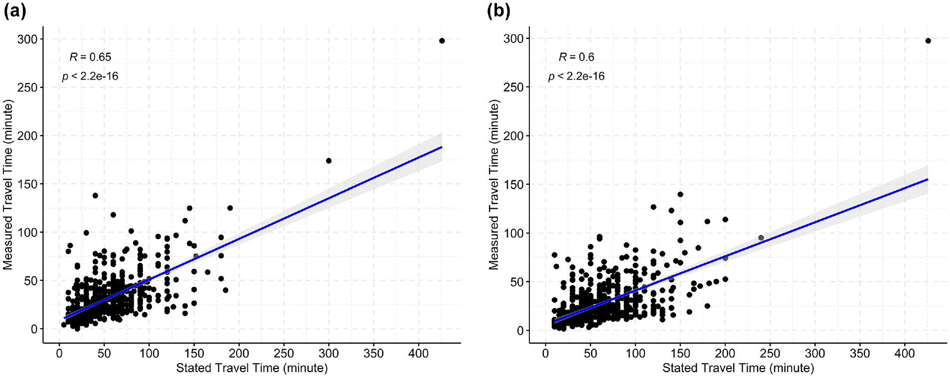
Correlation between stated and measured travel time: (a) home-to-work trip, (b) work-to-home trip.
Accounting for Schedule Delay
Schedule delay, which captures the disutility caused by traveling at times other than the desired time of travel, is a key variable in modeling departure time choice. Usually, the actual departure and travel times are recorded in RP surveys and the preferred arrival time (PAT) and preferred departure time (PDT) are missing from the data source. Asking direct questions to extract the information can also be biased given potential subjective justification toward the actual or the intended arrival time (i.e., respondents may try to justify to themselves and/or the interviewer that their actual behavior is the optimum). Different studies have used different modeling approaches to model schedule delay. Koppelman et al. ( 25 ) assumed that PDT follows the same trend as the observed departure time. Though this assumption could be realistic for air travelers, for regular commuters, it could be rigid. Ben-Akiva and Abou-Zeid ( 24 ) suggested two methods: (i) assumption of a constant desired time of travel by market segment as PDT and (ii) assumption of a latent desired time of travel assuming a probability density function for the latent (unobserved) PDT. While these methods yield good results in cities with homogeneous starting times of offices and businesses, the situation in Dhaka (as well as many other countries in the Global South) is more complicated. For instance, in the RP data used in the current study, the occupations are reported in three categories: public, private, and business (i.e., self-employed). However, depending on job type, the starting time of offices and the working hours very often vary within a single market segment. For example, in Dhaka, the opening times of public banks, administrative offices, and so forth is 10:00 a.m., whereas public universities, schools, and colleges have different start times. Therefore, it is not worthwhile to consider a constant time for a specific market segment in such a complex situation. Therefore, this study considered a latent desired time of travel for each market segment and the parameters of the distribution of the PDT were estimated along with the other model parameters.
Theoretical Model
The modeling framework is based on the random utility framework. Random utility theory suggests that individual decisions follow rationality and complete information. Decision-makers choose each alternative time with the highest utility, where the utility of an alternative

where, xin is the vector of the attribute of alternative
McFadden ( 26 ) proposed that this utility has the linear-in-parameters separable form:

where

where TTi is the travel time at alternative i. The early and late schedule delay can be defined as:

and

where PDTn is the PDT and DTi is the midpoint of the departure time interval of alternative time i measured in hours (e.g., for the 07:00 to 08:00 time interval DT corresponds to 07:30). In the absence of PDTn in the available RP data, statistical distributions are used. From a behavioral perspective, it is assumed that the disutility of earliness and lateness is lower around the PDT and higher when departure time spreads further away from the PDT. Therefore, it is assumed that the schedule delay is symmetrical for earliness and lateness and follows a parabolic function (as this functional form gives better consistency [ 23 ]). After adjusting the schedule delay term, the deterministic part of the utility equation can be expressed as:

where
Different assumptions about the distribution of the unobserved error term
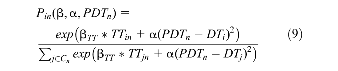
where
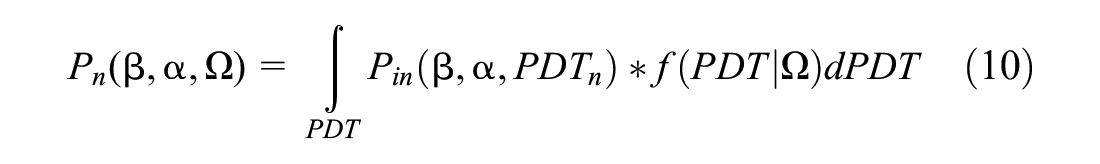
Since Equation 10 does not have a closed-form, a simulated log-likelihood is used using “Halton draws” from the specified distribution (normal distribution for Johnson’s distribution and uniform distribution for truncated normal distribution) to calculate the logit probabilities, which are then averaged over the number of draws. To keep the simulation variance lower in the estimated parameter and, at the same time, to reduce the computation run time, Halton draws have been used. The number of draws has been gradually increased starting from 50 till they were found to be stable for different starting values. The final model was estimated with 300 Halton draws ( 28 ).

Here,

where R is the number of draws and
Results and Discussion
Models have been estimated using the “Apollo” package R, applying the Maximum Likelihood Estimation with the BFGS optimization algorithm ( 30 ). Model estimation is done for both outbound and return commuting trips separately. Base outbound and return models are developed first, which are simple MNL models. The base models are then extended to advanced MMNL models that acknowledge the heterogeneity in PDT. Both in the base and advanced MMNL models, the effects of different socio-demographics have been considered. These effects are allowed to vary among the alternative time periods. It is important to note that, in the survey data, respondents who work at the office have been categorized as public and private employees and no further details about their professions have been recorded. These two categories are aggregated to a single category (“office employees”) as the choices of both car and ride-hailing commuters (who are likely to be “white collar” workers) are being modeled. Developed outbound and return models (both MNL and MMNL) include three broad types of independent variables: individual socio-demographics, household-level socio-demographics, and level-of-service attributes. Individual socio-demographic variables included in the model are: gender, usage of ride-hailing service (include Uber or Pathao car use and considered as a proxy of car availability), observed activity duration (<3 h or not). Since employees’ job flexibility information was missing from the data, observed activity duration is included as a dummy variable to capture its effect on the departure time choice. Household socio-demographics explored in the model specification include a dummy variable for income (household income >60,000 Bangladeshi taka [BDT] per month or not). The level-of-service attribute includes travel time which is estimated for different alternative periods where the observed and unobserved travel times have been calculated using the sub-model described in the Calculation of Travel Time section. To distinguish the influence of different occupations, in the outbound and return MMNL models different distributions of PDT have been defined. The modeling results from the outbound (home-to-work) and return (work-to-home) models are shown respectively in Tables 4 and 5. The signs of the parameter estimates are plausible; they support the hypotheses and are consistent with those in previous studies. Most of the variables considered are statistically significant at 95% confidence interval (Tables 4 and 5). However, for some parameters which are not statistically significant, corresponding coefficients have been retained in the model for the sake of comparison between simple MNL and MMNL models, and intuitive interpretation of each coefficient.
Estimates from Simple Multinomial Logit [MNL] Model and Advanced Mixed Multinomial Logit [MMNL] Model of Home-to-Work Trip.
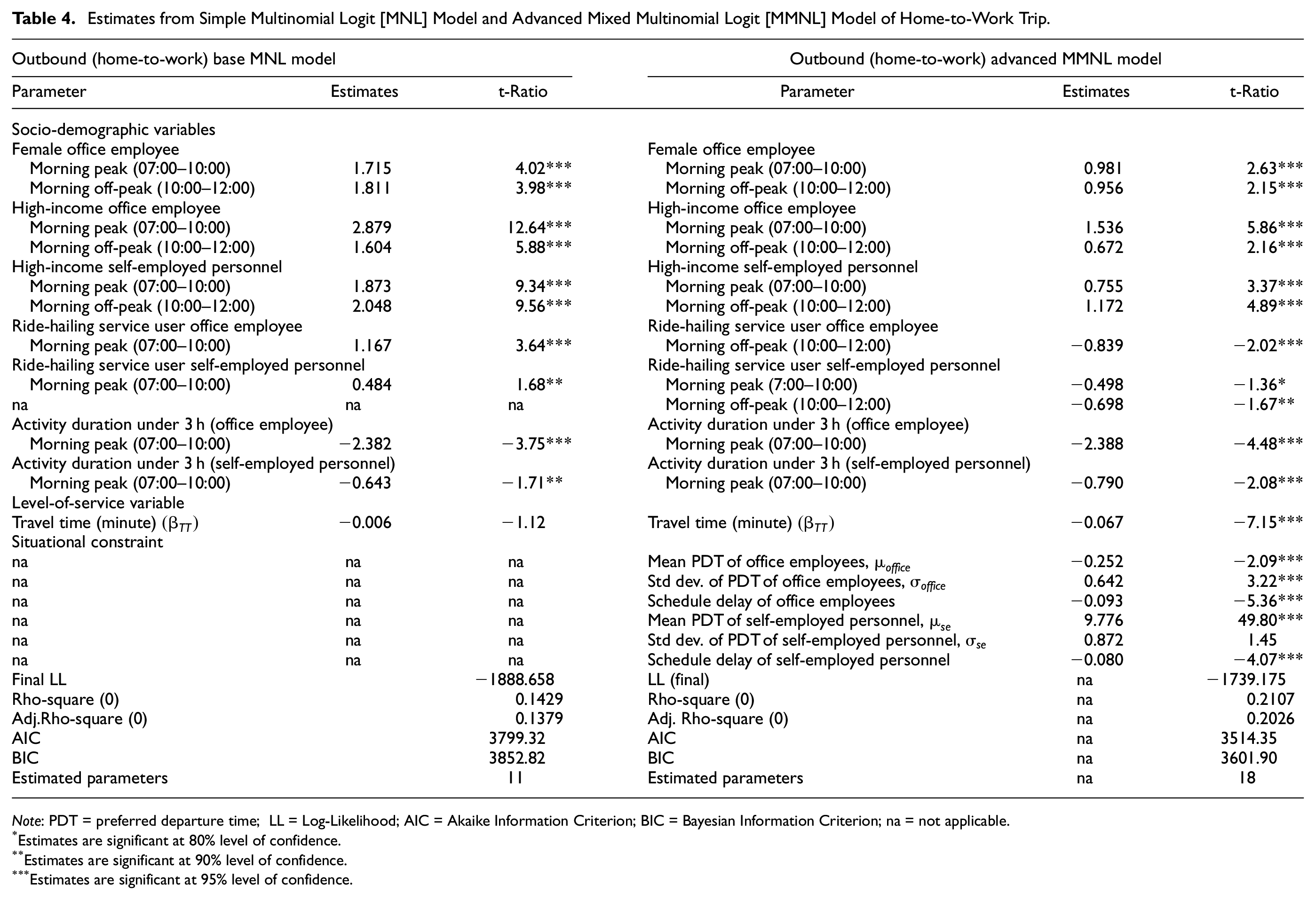
Note: PDT = preferred departure time; LL = Log-Likelihood; AIC = Akaike Information Criterion; BIC = Bayesian Information Criterion; na = not applicable.
Estimates are significant at 80% level of confidence.
Estimates are significant at 90% level of confidence.
Estimates are significant at 95% level of confidence.
Estimates from Simple Multinomial Logit [MNL] Model and Advanced Mixed Multinomial Logit [MMNL] Model of Work-to-Home Trip.
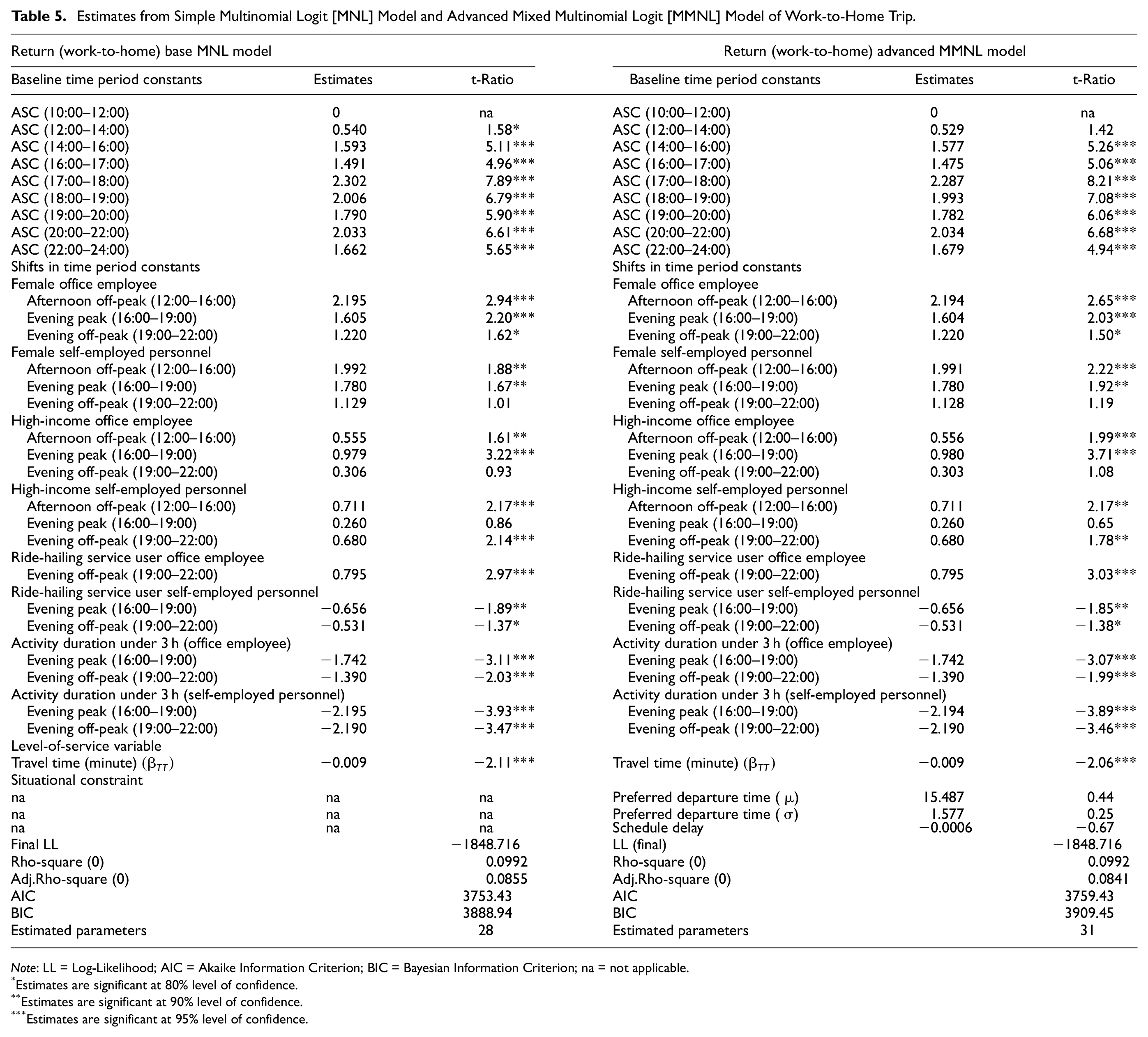
Note: LL = Log-Likelihood; AIC = Akaike Information Criterion; BIC = Bayesian Information Criterion; na = not applicable.
Estimates are significant at 80% level of confidence.
Estimates are significant at 90% level of confidence.
Estimates are significant at 95% level of confidence.
Outbound Model
For the outbound model, 10 discrete time intervals are grouped under four broad discrete time intervals: early morning (before 07:00), morning peak (07:00–10:00), morning off-peak (10:00–12:00), afternoon off-peak (12:00–16:00) and evening (after 16:00). These groupings are done considering the sign and magnitude of more disaggregate time-period-specific parameters.
Overall, most of the socio-demographic variables considered in the two specifications of the outbound models show similar trends. It is observed that different socio-demographic determinants have a significant influence in determining the departure time choice of car commuters for their home-to-work trips. For example, the results from both outbound models show that, compared with male commuters or female self-employed personnel, the utility associated with departing for the outbound trip is larger for the morning peak (07:00–10:00) and morning off-peak (10:00–12:00) for female office commuters compared with early morning, afternoon off-peak and evening (Table 4). This is intuitive given the potential consequence of increased obligation of housework and safety concerns (the majority of the cars in Dhaka are driven by male chauffeurs). A similar trend is observed in both models for office commuters with monthly income greater than 60,000BDT—the utility of departure for outbound is highest during the morning peak which is followed by morning off-peak time compared with the other periods. On the contrary, for self-employed personnel with monthly income greater than 60,000BDT the utility is highest during the morning off-peak followed by the morning peak. This implies the greater privilege of self-employed personnel to avoid peak time congestion and travel in the period of reduced travel time. In both models, office commuters and self-employed personnel who have activity durations less than 3 h have the lowest utility to travel during the peak time. The influence of observed activity duration can be explained by shorter activity durations (<3 h) implying the flexibility of employees both at work and at home. The effect of travel time is captured using generic coefficients for all time periods in both specifications. In both cases, the coefficient of travel time is negative, as expected, indicating disutility associated with longer travel times. The variable travel time is statistically not significant in the MNL model, but significant in the MMNL model. Therefore, it has been retained in the MNL model.
The MNL and MMNL specifications however lead to different sensitivities between car and ride-hailing service users. In the MNL specification, all else being equal, the office employees using ride-hailing services tend to prefer to travel in the morning peak time (07:00–10:00). Once the effect of schedule delay and PDT are accounted for in the MMNL specification, however, they show disutility associated with traveling in the morning peak compared with other alternative time period.
It may be noted that the influence of other socio-demographic variables (e.g., age, household size, vehicle ownership, etc.) have also been tested in both specifications, but not included in the final models as their influences are not significantly different from zero. Similarly, the effects of ASCs have been also tested, but not found to be statistically significantly different from zero.
In the MMNL model, the inclusion of schedule delay leads to a significant gain in model fit. The negative coefficient of the schedule delay term captures the increased disutility associated with a late arrival (i.e., after the start of office hours). The coefficient is statistically significant for both occupation groups, but sensitivity to schedule delay is slightly higher for the office employees (β = −0.09361) compared with self-employed personnel (β = −0.07999). The density curve of the PDT derived from the outbound MMNL model outputs shows a single peak for office employees with a mean value of approximately 09:00 (Figure 2a). On the other hand, for self-employed personnel, the PDT graph is similar to that for office employees (Figure 2b) with a slight shift of mean value toward the right (around 10:00). This can be explained by self-employed personnel being able to avoid office peak hours because of their increased flexibility and lower sensitivity to schedule delay. Further, higher sensitivity to schedule delay among office employees is attributed to the strict enforcement of the reporting time at the workplace (i.e., requirement to sign-in on arrival) compared with the more flexible schedule of self-employed personnel. It may be also noted that the corresponding standard deviation is statistically significant only among the office employees. This can be attributed to the start times (and subsequently reporting times) of office employees working in the public and private sectors being different (it was not recorded in the data whether or not an office employee worked in the public or private sector).
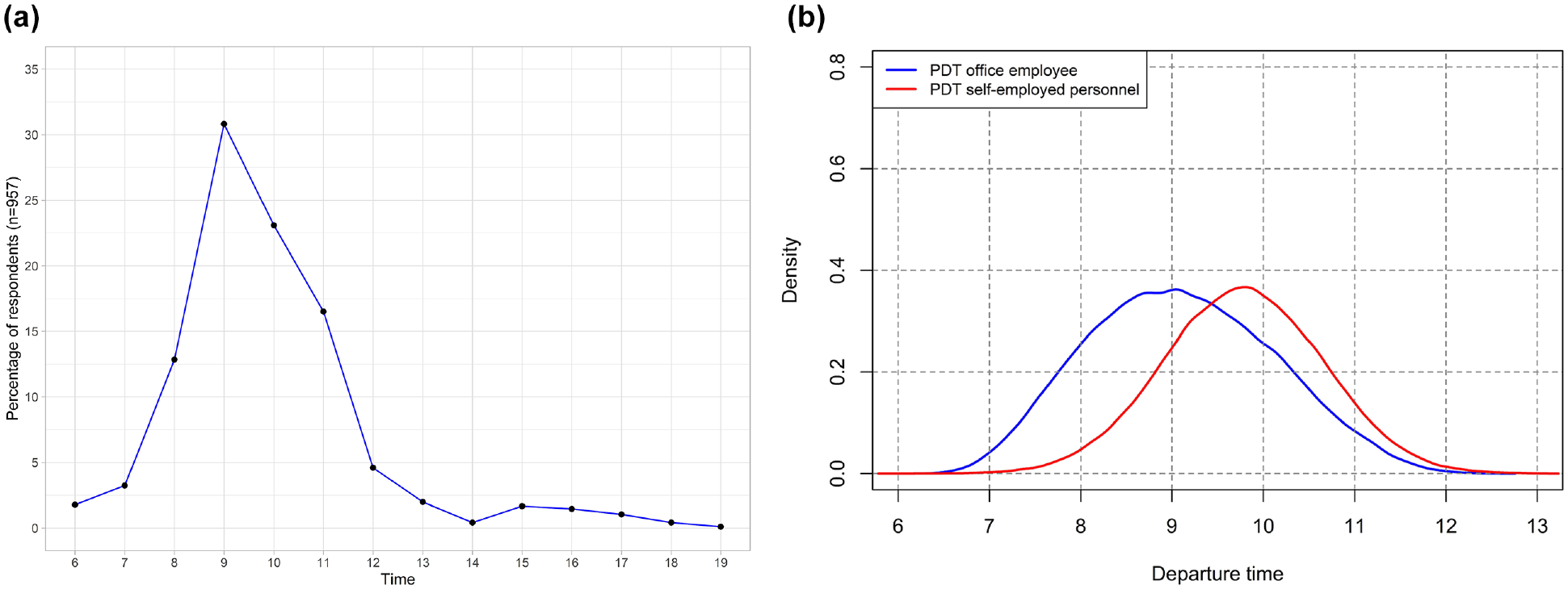
Home-to-work trip: (a) Observed departure time; (b) Preferred departure time.
Return Model
Table 5 summarizes the estimation results of the return model. In the return model, nine discrete time intervals are considered in the choice set: 10:00–12:00, 12:00–14:00, 14:00–16:00, 16:00–17:00, 17:00–18:00, 18:00–19:00, 19:00–20:00, 20:00–22:00, and 22:00–24:00. Unlike the outbound model, the ASCs of most of these time intervals are found to be significantly different from zero, therefore they were retained in the model. Results from both MNL and MMNL specifications indicate that, all else being equal, the most preferred time period is 17:00–18:00, followed by 20:00–22:00, 18:00–19:00, 19:00–20:00, 22:00–24:00, 14:00–16:00, 16:00–17:00, and 12:00–14:00 compared with the base alternative (10:00–12:00).
Similar to the outbound model, the return choice set is further grouped under four broad discrete time intervals: morning off-peak (10:00–12:00), afternoon off-peak (12:00–16:00), evening peak (16:00–19:00) and evening off-peak (19:00–22:00) to capture the heterogeneity associated with departure time choice among different socio-demographic groups. The same set of socio-demographic variables tested for the outbound trips have been tested in this regard. All the socio-demographic variables considered in the two specifications of the return models (MNL and MMNL) show similar trends. Estimated shifts in the time period parameters indicate that for both specifications, the utility for departing during afternoon off-peak (12:00–16:00) and evening peak (16:00–17:00) is higher for female commuters. This might be because traveling later (i.e., 19:00–22:00) can be associated with safety concerns, and returning before 12:00 is not likely to be feasible.
With regard to the availability of a personal car for return trips, the differences in preferences are tested separately for office workers and self-employed people. The shifts in the time period parameter estimates are statistically significantly different between the office employee and self-employed personnel, possibly because of the higher rate of car ownership (and therefore lower propensity to use ride-hailing services) among the self-employed personnel. The estimates reveal that office employees are more likely to choose evening off-peak time (19:00–22:00) for return trips if they are using car-based ride-hailing services. This is likely to be driven by the propensity to avoid the peak surcharge.
With regard to income, from both MNL and MMNL model specifications, it is found that for the office employee group with monthly income greater than 60,000BDT, the utility of returning is highest during the evening peak followed by the afternoon off-peak and evening off-peak. On the other hand, for the self-employed personnel who have monthly income greater than 60,000BDT, the utility is highest for departing at afternoon off-peak followed by evening off-peak and evening peak compared with other alternatives. This is likely to be associated with the higher flexibility of schedule of the self-employed group.
For office commuters and self-employed personnel who have observed activity duration less than 3 h, the utility for traveling during the peak time (16:00–19:00) is the lowest. The disutility of longer travel time of peak period might have exceeded the utility associated with short duration activity participation.
Unlike the outbound model, travel time coefficient is a significant determinant in both the return trip MNL and MMNL models. However, it is evident that the travel time parameter has a greater influence on the outbound trip (β =−0.06737 in the MMNL model) than the return trip (β =−0.009347 in the MMNL model). This suggests that car commuters are less willing to spend longer time in traffic for outbound trips than on their return trips.
Unlike the outbound MMNL model, the inclusion of situational constraint on the return MMNL model does not lead to a statistically significant improvement in the model fit and the coefficient of schedule delay is not statistically different from zero. This can be attributed to the greater flexibility in schedule during the return segment. The parameters of the PDT distribution (mean and standard deviation) are also not found to be statistically significant reflecting this flexibility. In the return segment, the MNL model outperforms the MMNL model, however, the density curve of the PDT derived from the return MMNL model is consistent with the reality (Figure 3b). It is also observed that the sensitivity to schedule delay is generally higher during the outbound trip than the return trip. This is intuitive because late arrival at the office probably has more serious consequences or penalties than late arrival at home. Overall, the model fit of the return model has lower R-squared value compared with the outbound model, which might be because of the many alternatives (times) considered in the model specification. Since inclusion of situational constraint on the return MMNL model does not improve the model performance, this study recommends the MNL model for the return segment.
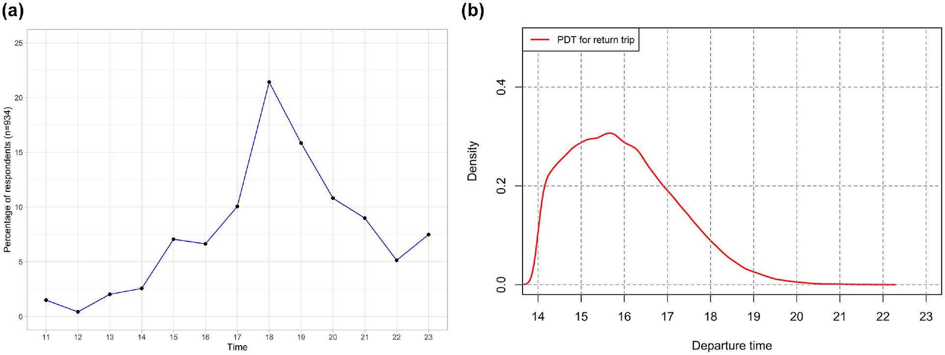
Work-to-home trip: (a) Observed departure time; (b) Preferred departure time.
Time Value of Schedule Delay
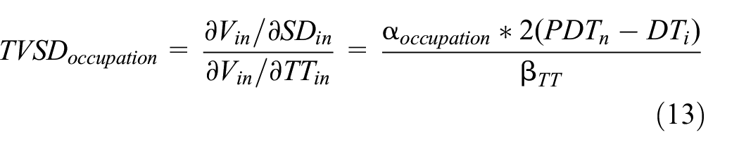
Generally, commuters encounter scheduled disutility with early arrival or late arrival at the workplace. Therefore, commuters attempt to choose the appropriate departure time by making a trade-off between travel time and schedule delay. For instance, they can choose the alternative with the “best travel time but large schedule delay” or “worst travel time with no schedule delay” or anything in between. To gain better insight from the developed model, therefore, the time valuation of schedule delay (TVSD) was estimated to understand the sensitivities to schedule delay versus travel time. TVSD is estimated using the formulation proposed by Bwambale et al. ( 23 ). It is estimated as the ratio of the partial derivatives of utility equation (Equation 8) with respect to schedule delay and travel time. The following equation has been used and the average of the estimated output is shown in Table 6. Since the schedule delay term is insignificant for the return trip, TVSD is only estimated for the outbound trip.
Time Valuation of Schedule Delay
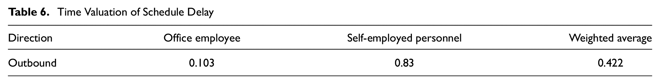
The estimated TVSD is the unitless metric representing the amount of delay a commuter is willing to experience for a unit reduction in travel time. The TVSD is lower for office employees than for self-employed personnel. This value signifies that office employees have very low willingness to accept schedule delay, potentially because of the very inflexible working hours in the office. On the other hand, self-employed personnel have the flexibility to choose longer schedule delay for the sake of reducing travel time. It may be noted that it was not possible to validate these because of absence of supplementary source of information. However, according to the literature, the TVSD in European countries varies between 0.81 and 1.71 ( 31 ). Therefore, the estimated output seems logical as the time valuation in developing countries will be lower than in developed countries.
Policy Insights
The estimated model parameters can be utilized in formulating peak-spreading policies for car travel in Dhaka, Bangladesh. Some proposals are suggested in this regard, below:
The coefficients of gender reveal that female office employees have a higher propensity to travel by car during the morning and evening peak hours. Targeted incentives for female employees (e.g., flexibility of start times, working from home privileges, discounted transport cost during the off-peak and/or public transport, etc.) could be taken into consideration.
The coefficients of income reveal that high-income office employees (household income >60,000BDT per month) are more likely to choose the peak time to travel when the schedule delay is minimum, but travel time is worst. This same group has higher affordability and therefore are less likely to be price sensitive. Therefore, a congestion pricing policy targeting the peak-time traveler, though an effective way for revenue generation, may not be effective to shift this group from traveling in the peak time. This revenue could, however, be a useful means of funding efficient and dependable public transport services.
The propensity to travel during the peak and off-peak time is very subtle for the users of ride-hailing services (e.g., Uber, Pathao Car). Changing the pricing structure of ride-hailing services to make peak-time travel much more expensive compared with the off-peak could serve as the incentive to travel during the off-peak time.
The higher sensitivity to schedule delay of the office employees and their lower willingness to accept schedule delay (i.e., lower time value of schedule delay) reflects the strictness of their schedules. Therefore, enhancing the flexibility of working hours of office employees (e.g., staggered start and end times, flexible start times, etc.) is a critical pre-requisite before the implementation of congestion pricing policies. To do so, the transport authority can work in collaboration with employers to estimate the required ratio of employee needed at a time in the office premises and offer flexibility to the rest so that they can travel during the off-peak time if needed.
The schedule delay was not found to have a significant effect on work-to-home trips. Therefore, the afternoon peak is likely to be easier to flatten compared with the morning peak.
Conclusion
In this research, the key challenges in modeling the departure time choice model in the context of Dhaka, Bangladesh, have been identified and solutions have been proposed. Separate departure time choice models of home-to-work and work-to-home of commuters using personal car/ride-hailing service have been developed to demonstrate the proposed solution to overcome the limitations of using RP data in modeling departure time choice. The methodological contributions include the following:
A new method to estimate the travel time for the full range of alternative time periods using Google Maps API and stated travel times when the Google Maps API is not deemed to be a reliable stand-alone source of travel time information.
Extension of the state-of-the-art method for representing PDT. Instead of assuming a constant value for a specific market segment or a generic statistical distribution, the proposed method includes two different statistical distributions for office workers and self-employed people acknowledging the high level of heterogeneity between and within each group. The estimation results support the hypothesis that a significant difference exists among different occupation groups in their departure time choices.
Based on the results, an advanced MMNL model is recommended for outbound trips to account for the heterogeneity in schedule delay among the travelers. A simple MNL model was found to be adequate for return trip segment where the schedule delay was not found to have a significant effect. The key aspects of the study are listed below:
The estimation results provide empirical evidence that departure time choices in Dhaka are significantly affected by activity duration, and schedule delay in addition to travel time. The results also reveal substantial heterogeneity depending on the type of job.
The results indicate that PDT/PATs, though unobserved in the RP data, are important aspects of departure time choice models. The proposed modeling framework to estimate the unobserved PDT through the assumed distribution parameters (mean and standard deviation) using a mixed logit framework can be an effective way to address the unobserved PDT issue, even in cross-sectional data. The framework can be also applied in case of passively generated data sources (e.g., GPS, mobile phone data, etc.) which also have the unobserved PDT problem.
Along with the distribution parameters, the sensitivities to schedule delay of different occupation groups have been estimated, which can be critical inputs in designing effective peak-spreading policies in Dhaka city. Results highlight that schedule delay and PDT parameters are significant in the home-to-work trip, but not in the work-to-home trip segments. This finding can have important policy implications.
Further, results suggest that car commuters are sensitive to travel time for both outbound and return trips. Therefore, policies aiming to reduce traffic congestion, such as road pricing, inbound flow control, and so forth, will enable commuters to adopt their PDT at the expense of minimal schedule delay.
Results indicate that schedule delay is the dominant factor for home-to-work trips and that the time value of schedule delay is much less compared with European countries (i.e., a commuter is willing to accept fewer units of schedule delay per unit reduction in travel time). The effect of income (high-income office employee dummy) is found to be more substantial than that of gender (female office employee dummy) for the home-to-work trips—but the trend is the opposite in the case of the return trip. The results thus strengthen the notion that there are problems associated with transferability of the models between developed and developing countries.
It may be noted that the effect of travel cost has been explored as well. Travel cost was not recorded in the data, however, and—in the absence of information about the vehicle type and the type of driver (as noted above, in Dhaka most cars are chauffeur-driven; there can be substantial variation in cost depending on the skill level of the chauffeur)—it was not possible to estimate the cost in a reliable manner. This can be explored in future using primary data or appropriate supplementary data. Further, the current study focuses only on commuting trips made by car, which are the biggest contributors to traffic congestion in Dhaka. In future, this could be extended to commuting trips made by public transport and paratransit modes, and include other trip purposes.
However, even in the current form, the research findings can be practically useful for devising peak-spreading policies in Dhaka—either as a stand-alone tool to test the impact of varied start times of offices in different locations or within an agent-based simulation tool to test the impact of different congestion pricing policies. In addition, the proposed framework could be useful in other developing countries with similar data issues.
Footnotes
Acknowledgements
The authors acknowledge the help from Mr Anisur Rahman and Mr Dhrubo Alam of DTCA for providing clarifications with regard to the data.
Author Contributions
The authors confirm contribution to the paper as follows: study conception and design: K. Zannat; data collection: K. Zannat, C. F. Choudhury; analysis and interpretation of results: K. Zannat, C. F. Choudhury, S. Hess; draft manuscript preparation: K. Zannat. All authors reviewed the results and the responses and approved the final version of the manuscript.
Declaration of Conflicting Interests
The author(s) declared no potential conflicts of interest with respect to the research, authorship, and/or publication of this article.
Funding
The author(s) disclosed receipt of the following financial support for the research, authorship, and/or publication of this article: The funding for the research has been provided by the Faculty for the Future Program of the Schlumberger Foundation. Charisma Choudhury’s time has been partially supported by the UKRI Future Leader Fellowship (Grant Number MRT020423/1).
Data Accessibility Statement
The data used for the study has been made available by the Dhaka Transport Coordination Agency (DTCA).