Automated Assessment of Passing Sight Distance on Rural Highways using Mobile LiDAR Data

Abstract

Providing sufficient Available Sight Distance (ASD) that meets the minimum design requirements is crucial for highway safety. Previous work on sight distance assessment focused on Stopping Sight Distance (SSD) with little attention given to Passing Sight Distance (PSD). Insufficient PSD could lead to severe collisions such as head-on and sideswipe crashes. To address this gap, this paper introduces an automated method for PSD assessment on two-lane highways using mobile Light Detection and Ranging (LiDAR) data. The procedure involved extracting centerline lane marking, defining passing-allowed and passing-prohibited regions, computing the ASD, and comparing the existing centerline marking pattern (i.e., passing and no-passing zones) to a proposed lane marking that is based on the ASD for passing maneuvers. Regions that meet the design standards, substandard zones, and non-optimal design regions were all defined. A reallocation of PSD zones was conducted based on the ASD including modifying the existing lane marking pattern, which resulted in increasing the total length of passing zones by up to 20%, providing more, but safer, passing opportunities. A high-level safety assessment of historical collisions showed clusters of crashes along regions where passing is currently allowed at locations where the ASD is less than standard requirements. The proposed framework represents a tool by which transportation agencies could assess PSD, upgrade the design of existing highways, and investigate the consequences of PSD limitations to ensure compliance with standards during highway service life.

The Available Sight Distance (ASD) is a core element when designing highways to ensure a safe driving environment ( 1 ). Different types of sight distance are accounted for in the design stage, including Stopping Sight Distance (SSD), Passing Sight Distance (PSD), Non-Stripping Sight Distance, and Decision Sight Distance, with SSD and PSD being the prime aspects of sight distance. The American Association of State Highway and Transportation Officials (AASHTO) defines SSD as the total of perception-reaction and braking distances needed by a driver to realize the presence of a potential hazard and come to a safe and complete stop ( 1 ). The PSD is the distance required by a vehicle to safely complete a passing maneuver on two-lane two-way highways where passing is permitted. To ensure drivers’ safety, highway design standards necessitate that ASD is greater than the minimum requirements for the expected maneuver, whether it is stopping or passing ( 2 ). Unfortunately, the failure to meet the minimum sight distance requirements leads to limited vision for drivers, which could be associated with more traffic collisions. Thus, maintaining adequate SSD and PSD during the service life of a highway is of crucial importance for safe highway operation.

Previous studies showed that sight distance deficiencies affect traffic safety and operation efficiency on highways ( 3 , 4 ). Limiting a driver’s vision is considered a contributing factor in collision occurrence along road corridors and construction sites. A previous study on evaluating the safety of construction fatalities between 1990 and 2007 concluded that the absence of sufficient sight distance was a primary cause for about 5% of total crashes at these sites. It was also shown that when a vehicle is involved in a collision, over 23% of those collisions were caused mainly by the presence of obstructions ( 5 ). In such cases, recommended measures usually include identifying sight obstacles and defining proper mitigation strategies based on hazard type and available budget. Therefore, improving the safety of locations where sight distance is limited relies mainly on locating obstructed areas and identifying hazards. This requires detailed field measurements of the ASD to serve as a basis for proposing and implementing effective safety measures.

ASD can be evaluated using various methods, which can be classified into two categories: (i) two dimensional (2-D) methods; and (ii) three dimensional (3-D) approaches. When using 2-D methodologies, sight distance is usually assessed during sight visits, where professionals use traditional surveying methods to collect information on road segments where the vision is obstructed. Using 2-D-based methods is associated with several limitations. First, the ASD is often evaluated separately on the horizontal and vertical alignments ( 6 ). Since the ASD relies on various road geometric attributes, roadside features, and the integrated effect of horizontal and vertical alignments, computing the ASD using 2-D projection could be inaccurate. Previous work found that combined road vertical and horizontal alignments have concurrent effects on ASD and impose more vision restrictions, which led researchers to conclude that considering both alignments when assessing ASD is a more reliable approach ( 6 , 7 ). Second, the conventional field measurement of ASD could represent a safety concern as it requires personnel to be in or adjacent to active traffic lanes when data is collected. Third, using traditional sight distance assessment methods, especially on a large scale, is time-consuming, labor-intensive, and could be an infeasible process because of the considerable manpower required depending on the road network size.

To overcome limitations associated with conventional methods, recent research has introduced various technologies to provide 3D-based assessments of sight distance on highways. In this approach, different information sources such as Global Positioning System (GPS) data, Geographic Information System (GIS) maps, and Light Detection and Ranging (LiDAR) data are used. The majority of GIS-based sight distance calculation applications focused on assessing the ASD using ArcGIS tools ( 8 ). Although this has been very useful in shifting the attention to the use of 3-D models of highways, it still requires considerable manual input during different phases of the assessment process, which hinders large-scale implementation and makes the aggregate assessments desired by transportation agencies infeasible. With the recent advances in remote sensing and the noticeable power of using remotely sensed data sets, attention has been shifted to using LiDAR data as 3-D models for sight distance computation. Several benefits support the emerging popularity of using LiDAR data. The acquired LiDAR dataset can be used for various purposes such as extracting road features, assessing sight distance, analyzing site conditions, conducting safety reviews, and transportation studies ( 9 – 18 ). Moreover, many transportation agencies have begun to obtain mobile LiDAR data to map their roadway assets and gain access to 3-D models of their road networks enabling frequent, and virtual visits from the safety of their offices ( 19 ).

The majority of previous studies on developing sight distance assessment tools focused on SSD with less attention given to PSD ( 10 , 20 ). Passing is a risky maneuver in which a sufficient ASD needs to be ensured to provide a vehicle a safe opportunity to pass another slowing vehicle ahead using the lane of the opposing traffic. The failure to provide sufficient sight distance at locations where passing is permitted could result in severe collisions such as head-on, sideswipe, and run-off-road crashes ( 21 ). Compared with SSD-related collisions, which likely result in Property Damage Only (PDO), crashes associated with PSD limitations likely lead to fatalities ( 21 ). With the previous studies being centered on studying SSD and the severity of collisions that result from the failure to meet PSD requirements, there is a need to develop a robust methodology to assess the PSD on two-lane two-way highways and ensure that passing zones meet, and preferably exceed, the minimum requirements of design standards.

This paper, therefore, addresses these limitations and develops an automated method for assessing the 3-D sight distance available for passing maneuvers using mobile LiDAR data. The objectives of this research are: (i) to develop an automated tool to assess the sight distance available for passing maneuvers on highways; (ii) to use the proposed method to reallocate the existing lane marking based on the estimated ASD to ensure safe passing maneuvers by ensuring that adequate sight distance is available on exiting highways where passing is permitted, in other words, to use the outcome of the sight distance assessment tool and identify locations where passing should be permitted or prohibited in comparison with the existing lane marking configuration (i.e., whether passing is currently allowed or not); and (iii) to conduct a high-level safety review to explore if limited sight distance along passing zones on highways have likely resulted in PSD-related collisions in the past.

The procedure involves extracting centerline lane marking, defining passing-permitted and passing-prohibited zones, assessing ASD, and comparing the ASD with the minimum PSD required by design standards. The algorithm was tested on 16 km (≈9.94 mi) of LiDAR data of two-lane two-way highway segments in Alberta, Canada. The results showed that the code successfully defined passing-allowed and passing-prohibited regions and computed the ASD along test segments. The output of this work is a tool to be used by transportation agencies to evaluate PSD and improve compliance with design standards. The paper then makes recommendations for reallocating passing-permitted zones and proposes a new centerline marking pattern that provides more/fewer, but safer, passing regions. The paper also investigates the occurrence of historical collisions along regions where passing is currently allowed, but the ASD is found to be lower than the required PSD. To conclude, the framework presented in this paper represents a tool that could help transportation agencies involved in PSD assessments, design reviews, and upgrades of existing two-lane highways to conduct safety assessments of passing-related collisions.

Previous Studies

There have been several studies on assessing ASD on roadways. One of the earliest studies was conducted by Lovell ( 7 ), who developed parametric curves to represent the road centerline. These curves were then used to assess the ASD using 2-D projection. This method was recommended to be used on flat roadways since it does not consider the road vertical alignment. Hassan et al. ( 22 ) proposed a method to estimate the ASD along the roadway horizontal alignment. This method was also based on evaluating the sight distance against lateral obstructions without considering the roadway’s longitudinal profile.

Several researchers provided 2D-based methods for sight distance measurement, and some studies provided semi-automated algorithms to compute the ASD in a 3-D world. Ismail and Sayed ( 23 ) proposed an algorithm to calculate the 3-D sight distance based on a parametric representation of the roadway and roadside elements. The authors also examined the impacts of various road geometric attributes of sight distances. In other work, Nehate and Rys ( 6 ) estimated the ASD along roadways using GIS data. Road surface and obstructions were represented by piecewise parametric equations. Sight distance was then computed by searching for the conflict between sightlines and obstructions. The model was found to be of moderate accuracy because of its inability to consider bumpy vertical alignments. The ASD was also assessed by Castro et al. ( 8 ) using a GIS-based method.

The authors computed the sight distance on different highways using ArcGIS software. Their results were then compared with sight distance values estimated by road design software. The study concluded that there were some differences between the two methods, but they were not statistically significant. The road design software was also found to yield shorter sight distance values because of its ability to detect road vertical alignment. Moreover, Namala and Rys ( 24 ) proposed calculating the ASD using GPS data to identify the passing-prohibited zones. De Santos-Berbel et al. ( 25 ) compared using 2-D and 3-D sight distance assessment methods. The results of this study emphasized the importance of using 3D-based approaches, especially in traffic safety assessments. With the increasing popularity of using LiDAR technology, recent studies focused on using LiDAR point clouds in sight distance estimation. Castro et al. ( 26 ) proposed a method for sight distance computation using aerial LiDAR data and ArcGIS tools. The authors indicated that this method’s processing time was lower than that of a previous study ( 8 ). LiDAR data was also used by Khattak et al. ( 27 ) to define sight obstructions at intersections. The method proposed by the authors was able to identify 90% of the actual obstructions at studied locations. In 2015, Bassani et al. ( 28 ) conducted sight distance analysis using point clouds obtained through the conversion of collected photogrammetric images of a road segment. ArcGIS tools were then used to compute the ASD.

Recently, Gargoum et al. ( 20 ) introduced a semi-automatic approach for ASD assessment using ArcGIS tools and mobile LiDAR data. A script was written in Microsoft Visual Basic (VB) to process ArcGIS output and estimate the ASD. Locations with limited sight distances were defined. One of the challenges reported by the authors was the long processing time resulting from the high number of observer and target points. In a more recent study, Shalkamy et al. ( 10 ) developed an automated methodology to evaluate the SSD on different highway segments using mobile LiDAR data. The method involved assessing the ASD, comparing ASD values to the minimum requirements of design standards, and identifying locations with sight obstructions. The authors recommended future research to assess the PSD on highways.

The above review reveals that several studies have been conducted to assess the SSD on highways, with minimal attention given to evaluating PSD and its implications on road safety. The majority of the previous studies used 2-D-based approaches or proposed 3-D-based methods using ArcGIS tools that still require significant manual input and represent a challenge if a large-scale assessment is desired. As recommended in previous work, this paper introduces an automated method to assess PSD on highways using mobile LiDAR point clouds. The procedure used extracts centerline lane marking, defines regions where passing is permitted and others where it is prohibited, and assesses the ASD against passing requirements. Using a case study of highway segments, the developed method is used to explore whether passing-allowed zones meet the PSD requirements. The proposed framework could help Departments of Transportation (DOTs) assess and upgrade passing zones on their highway network and conduct safety reviews to gain more understanding of the potential causes of PSD-related crashes.

LiDAR Data

The data used in this paper are mobile LiDAR data collected by Alberta Transportation on numerous highways in Alberta, Canada. A laser scanning system (REIGL VMX 450) was used to collect 360° LiDAR point clouds representing 3-D models of scanned highways. Figure 1 shows a virtual image of the LiDAR point cloud for one of the highway segments. Information collected on points includes x, y, z, intensity, and scanning angle. LiDAR data were acquired using a data collection truck that scans highway segments while driving at the posted speed limits without causing any traffic disruption. The data obtained have a high density of an average of 300 points/m² on the pavement surface, and point intensity ranges from 2,000 to 67,000 with an average of 21,000. The data collected were stored in several LASer (LAS) files, each of which represents a 3-D model of a 4-km (≈2.49 mi) highway segment and contains up to 30 million points. Because of the high density of point clouds and the rich information contained, the size of an LAS file of a 4- km section could reach 700 MB. This large file size indicates that the LiDAR model is rich, containing a large amount of information about millions of points. This required storing the LiDAR data files on a secure Hard Drive of 3 TB capacity.

Figure 1.

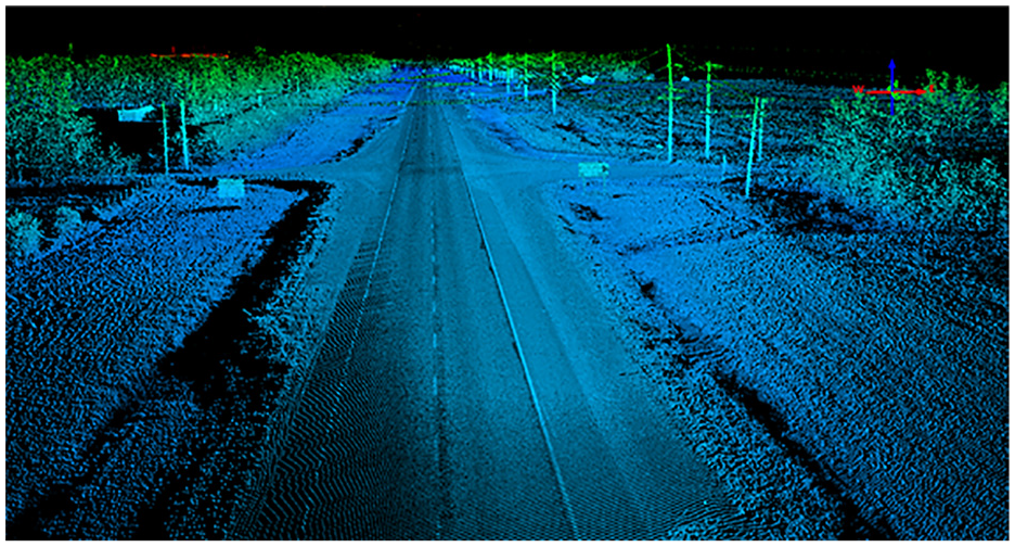
A virtual image of the LiDAR point cloud sample.

Mobile and airborne LiDAR are the most common data sources used in extracting information on roadways. Mobile LiDAR data are known to have higher point density, a good view of the road surface, and a better view of vertical surfaces such as the faces of roadside features and buildings but they cannot capture the tops of buildings. Airborne LiDAR data have a lower point density and a better view of pavements and building surfaces but have a poor view of vertical faces ( 29 ). Airborne LiDAR systems have a great advantage of providing a more synoptic view of scanned areas, however, such a wider coverage comes at the expense of lowered point density of collected data ( 30 ). This indicates that different data types have various advantages and disadvantages and can, therefore, be used for different purposes. For example, more detailed information about roadside features that could restrict a driver’s visibility can be obtained using mobile LiDAR data, while a wider coverage of scanning can be achieved through using airborne LiDAR data. Even though airborne LiDAR data can also be a potential source of data for ASD assessment, considering data availability and the above-mentioned advantages (including that ASD can be limited by roadside features or the vertical curvature of pavement surfaces that are better represented in mobile LiDAR data), this study uses mobile LiDAR data and imagery data sources that can be better used in a wide range of applications such as feasibility studies, mapping, vegetation planning, road alignment selection, and environmental assessment ( 31 ).

It is worth mentioning that a huge advantage in using mobile LiDAR data is that the same data set can be used for different applications which could potentially result in considerable money and time savings. The use of the same LiDAR data set in several applications could justify the investment in using LiDAR in transportation engineering. In fact, adopting LiDAR data in assessing and managing highway networks could open a new epoch of asset management, design review, and road safety audits.

Methodology

The procedure used has five stages: (i) extracting lane markings to identify passing-permitted and passing-prohibited zones; (ii) defining observer and target points which represent the driver’s eye and object locations at which the ASD is assessed; (iii) LiDAR point cloud voxelization in which LiDAR data are converted into a 3-D representation of a highway segment; (iv) estimating the ASD; and (v) comparing the ASD with the minimum requirements of PSD. These five stages are executed on test segments, after which the sight distance available for passing is compared with the pattern of the existing lane markings. This process is applied to ensure the compliance of existing conditions with design standards requirements and provide recommendations if substandard regions are found. A high-level preliminary safety review is also performed in which historical collisions, information on ASD, and patterns of existing lane marking are all mapped for further assessment. Figure 2 shows the workflow summarizing the paper framework. The following sections explain the applied method in more detail.

Figure 2.

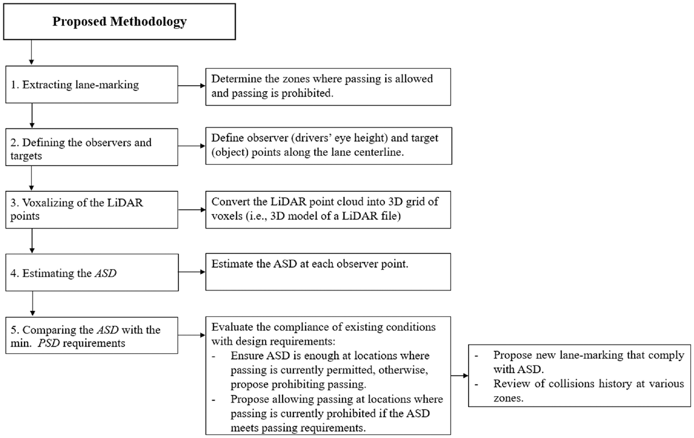
Overall workflow of the proposed methodology.

Lane Marking Extraction and Passing Zones Identification

These zones first need to be identified to estimate the ASD along the permitted/prohibited passing zones of a highway segment. Passing-allowed and passing-prohibited regions can be defined through the pattern of the centerline lane markings. When the centerline lane marking type is “dashed,” this refers to a passing-permitted zone, while regions with “solid” lane marking represent zones where the passing maneuver is prohibited. Thus, it is essential to extract lane marking information to define these regions.

The lane marking is extracted by applying two filters onto the LiDAR point cloud. The first filter uses the proximity to the vehicle trajectory. After reading LiDAR data with the algorithm, points representing the path (i.e., trajectory) of the data collection truck are extracted by filtering the data using the scanning angle. Previous research ( 10 , 12 ) showed that points scanned at a zero scanner-angle are located right under the laser scanner and represent the data collection truck’s trajectory. To optimize the number of points processed by the algorithm, the first filter is applied to extract all points near the trajectory points, which covers the limits of travel lanes. Since the paper focuses on passing maneuvers on two-lane two-way highways and the lane width of test highways ranges from 3.5 m (≈11.48 ft) to 5.0 m (≈16.40 ft), filtering the data to keep the points that are located at a distance between 2.5 m (≈8.20 ft) and 5.0 m (≈16.40 ft) would keep point clouds that cover the centerline lane markings. The second step involves using an intensity-based filter. LiDAR data contains information about points’ position, elevation, as well as intensity. Highly reflective objects, such as lane markings, have high-intensity readings. Since lane marking is the highly reflective object from the group of points previously filtered, the intensity filter successfully isolates lane marking from the pavement surface, as shown in Figure 3. Using sensitivity analysis revealed that intensity readings of lane markings in the analyzed segments range from 29,000 to 33,000. Thus, this range was used in the extraction process.

Figure 3.

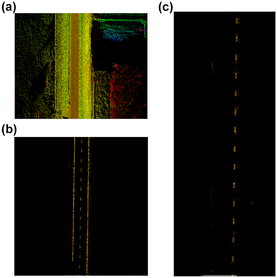
A visualized road segment before and after lane marking extraction: (a) all points; (b) the first filter output; and (c) the second filter output.

The next step is to use the extracted lane marking to determine passing-permitted and passing-prohibited zones. This involves separating centerline marking into two parts: (i) a proportion where the centerline lane marking type is “dashed,” which refers to a “passing-allowed” zone; and (ii) a proportion along which the centerline marking is a “solid” line (i.e., continuous) which represents a “passing-prohibited” zone. This is implemented by using a Density-Based Spatial Clustering of Applications with Noise (DBSCAN) clustering algorithm ( 32 ), which is an algorithm that groups points based on their proximity and hit count (i.e., density and number of points in each cluster). The proximity represents how close the points are to each other. The typical centerline lane marking consists of dashed lines (i.e., each of which is 3 m [≈ 9.84 ft] long) that are 6 m (≈19.69 ft) apart. Therefore, when setting the criteria of defining clusters of dashed lines, a threshold of 3 m (≈9.84 ft) (i.e., the typical dashed line length) is used. The hit count represents the number of points in a cluster. Considering the density of the LiDAR data used (300 points/m²) and the geometric properties of dashed marking lines, clusters that have between 10 and 100 points and a cluster length of up to 3 m (≈9.84 ft) are considered points of “dashed” marking lines, and those containing more than 100 points with a cluster length greater than 3 m (≈9.84 ft) are considered “solid” marking lines. Since the lengths of “dashed” and “solid” centerline marking lines are typical (i.e., have standard values) and significantly different, these criteria enabled successful lane marking extraction and passing zones identification on all analyzed highway segments. The output of this step is a graph that represents the lane marking along the test segments, as shown in Figure 4. This outcome will then be used in the results analysis section for each road segment.

Figure 4.

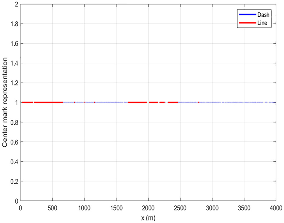
A sample of the algorithm output for the lane marking extraction.

Observers and Targets Definition

After extracting the centerline lane marking, the next step is to define the observer and target points. Observer points represent driver’s locations along the driving lane centerline for which the sight distance is to be assessed. Target points represent locations being observed by a driver along the roadway. In other words, targets are a set of points to be observed by observer points. Trajectory points of the data collection truck that have been extracted in the previous step (i.e., the points that lie on the path of the data collection truck) are, therefore, used to represent the observer and target points. The distance between observer and target points depends on the interval at which the sight distance is to be assessed. The ASD is typically assessed every 20 m (≈65.62 ft) to 50 m (≈164.04 ft) along highway segments ( 20 ). Sensitivity analysis showed that assessing sight distance at 5 m (≈16.40 ft) to 20 m (≈65.62 ft) distance intervals yields almost the same results. Although the user can alter the distance at which the ASD is estimated, this paper’s sight distance is computed every 20 m (≈65.62 ft). Therefore, the moving average technique is used to smooth the trajectory points and generate observer and target points that are 20 m (≈65.62 ft) apart. After the observers and targets are defined, their elevations are modified to comply with Alberta Highway Geometric Design Guide requirements ( 33 ) which recommend that, when the ASD is computed to evaluate PSD requirements, an observer height of 1.05 m (≈3.44 ft) and a target height of 1.30 m (≈4.27 ft) should be used. The outcome of this step is a vector that contains observer points o_i = [i, i+1, i+2, …., n] and a vector t_j = [j, j+1, j+2, …., m] that contains target points between each of which the ASD is to be calculated. As a validation step, the extracted set of points was mapped onto the LiDAR point cloud using Quick Terrain Modeler software ( 34 ) and found to be aligned perfectly along the driving lane along which the sight distance is evaluated.

Voxelization of LiDAR Data

The third stage includes creating a 3-D model of the highway segment to assess the sightlines in a 3-D view. Voxelization is based on a 3-D histogram counting algorithm ( 35 ). It is also the process of dividing the LiDAR point cloud into a 3-D grid of voxels of a size that can be altered by the user. In this step, the LiDAR point cloud is converted into voxels that are 3-D volumetric shapes (i.e., cubes) and represent the road segment. Using this approach, a point cloud file is divided into a 3-D grid consisting of millions of voxels with a unique identification number given to each voxel. The number of defined voxels depends on the size of the LiDAR point cloud and the voxel size defined by the user. The points contained in the point cloud are then assigned to the defined voxels based on their spatial coordinates. To demonstrate how a point is assigned into a voxel, let P(x, y, z) denote a point to be assigned to a voxel v (i, j, k) of dimensions Δx, Δy, and Δz in the x, y, and z directions. Let (x₀, y₀, z₀) denote the origin of the 3-D voxel grid. Then the spatial identification number of the voxel v (i, j, k) that would contain the point P (x, y, z) is computed as follows ( 36 ):

$$i=\frac{\mathrm{int}(x-x_0)}{{\Delta }_x}$$

(1)

$$j=\frac{\mathrm{int}(y-y_0)}{{\Delta }_y}$$

(2)

$$k=\frac{\mathrm{int}(z-z_0)}{{\Delta }_z}$$

(3)

For more information about the voxelization process, the reader is referred to a previous study by Gargoum et al. ( 36 ). It is worth noting that using voxelization to discretize LiDAR point cloud does not compromise information on objects in the 3-D space ( 37 ). It is a process by which discrete millions of points are assigned to a smaller number of 3-D shapes to be processed by the algorithm much faster. This step’s outcome is a 3-D grid of voxels representing the road segment, and it will be used as the 3-D input model for the next step, “estimating the ASD.”

Estimating the Available Sight Distance for Passing Maneuvers

To compute the ASD for passing at each observer, observers and targets are overlayed onto the grid of voxels created in the previous stage. The next step is to connect vectors representing sightlines from every observer to all targets included in the observer and target vectors previously defined. The algorithm starts at the first observer O_i (i=1) and connects vectors to all targets contained in the vector t_j (j=1:m). Suppose the first target is visible (i.e., no obstructing voxels exist along the connecting vector between the observer and the target). In that case, the code then moves to assess the successive target until the code detects the first obstructing voxel. Once the first obstructed voxel is defined, the ASD is recorded as the distance between the observer and the last visible target. A voxel is considered to be obstructing the sightline (i.e., sight vector) when the vector position is lower than the highest point’s position belonging to the voxel or higher than the position of the lowest point the voxel contains. The same assessment process is repeated at all observers along the passing-permitted and passing-prohibited regions while recording the ASD at each observer. The code then outputs the ASD along the entire segment, as shown in Figure 5. The last step uses LiDAR data of test segments and involves comparing the ASD with the minimum PSD required by the design guide, which depends on the design speed of the highway segment. This is followed by reviewing the existing pattern of centerline lane marking (i.e., current permission or prohibition of passing) with the resulting ASD to ensure compliance of existing highways with design standards and to propose improvements for allowing or prohibiting passing maneuvers based on the ASD and the pattern of existing lane marking.

Figure 5.

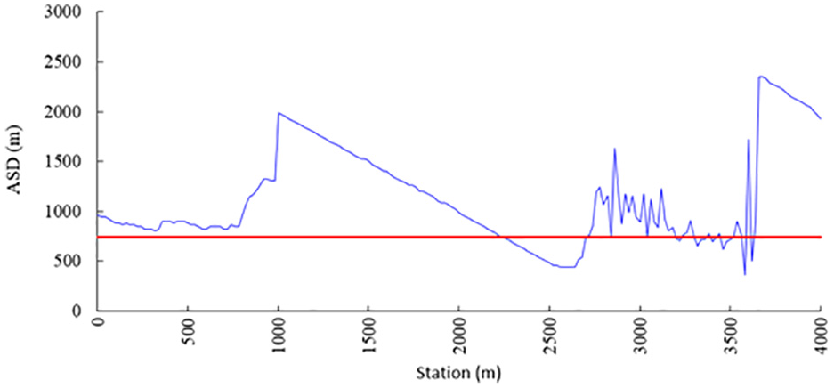
A sample of the algorithm sight distance assessment output.

The phases mentioned above have been implemented using MATLAB programming software ( 38 ). The methodology is executed through two MATLAB codes. The first MATLAB code starts by reading the LiDAR data file, then extracts the existing lane marking as explained previously. The second MATLAB script reads the same LiDAR file, defines the observers and targets, and then converts the LiDAR data into a 3-D grid of voxels. After that, the code overlays the observers and targets into the voxels and creates sightlines between each observer and all targets to estimate the ASD. The outputs of both MATLAB codes (graphs) are combined and then used to analyze the results.

Test Segments

The proposed procedure was coded using MATLAB. The developed algorithm was tested on LiDAR data from 16 km (≈9.94 mi) two-lane two-way highway segments. All segments are located on Alberta Provincial Highway No. 35 (principal arterial) located in the northwest of the Province of Alberta and designated as one of Canada’s National Highway System’s core routes. All segments are two-lane undivided rural highways. The Average Annual Daily Traffic (AADT) for these segments ranges between 1,065 and 1975 vehicles/day. The test sections are four highway segments, 4 km (≈2.49 mi) each, with varying horizontal and vertical alignment features and a balanced presence of passing-allowed and passing-prohibited zones. The posted speed limit is 100 km/h (≈62.14 mph), and the design speed is 110 km/h (≈68.35 mph). According to Alberta Highway Geometric Design Guide, the minimum required sight distance to perform a passing maneuver is 740 m (≈2,427.82 ft) according to the highway speed limit.

Results and Discussion

As discussed, the methodology involves five stages (Stage 1 to 5) as shown in Figure 2. This section discusses the results of executing the proposed procedure by applying the developed algorithm to the test segments.

Lane Marking Extraction (Stage 1)

The lane marking was extracted for the four segments to identify passing and no-passing zones, as shown in Figure 6 (i.e., the figures are the outputs from step 1 which is extracting the lane marking). As shown, lane marking was successfully extracted, and the proposed procedure defined passing-allowed and passing-prohibited regions. Passing zones, where a driver is allowed to pass a slowing vehicle ahead, are represented by dashed (i.e., blue) lines while solid (i.e., red) lines represent zones in which passing is not permitted. The original LiDAR data files were visually inspected to verify the code output, which perfectly matched the lane marking pattern in the original LiDAR data.

Figure 6.

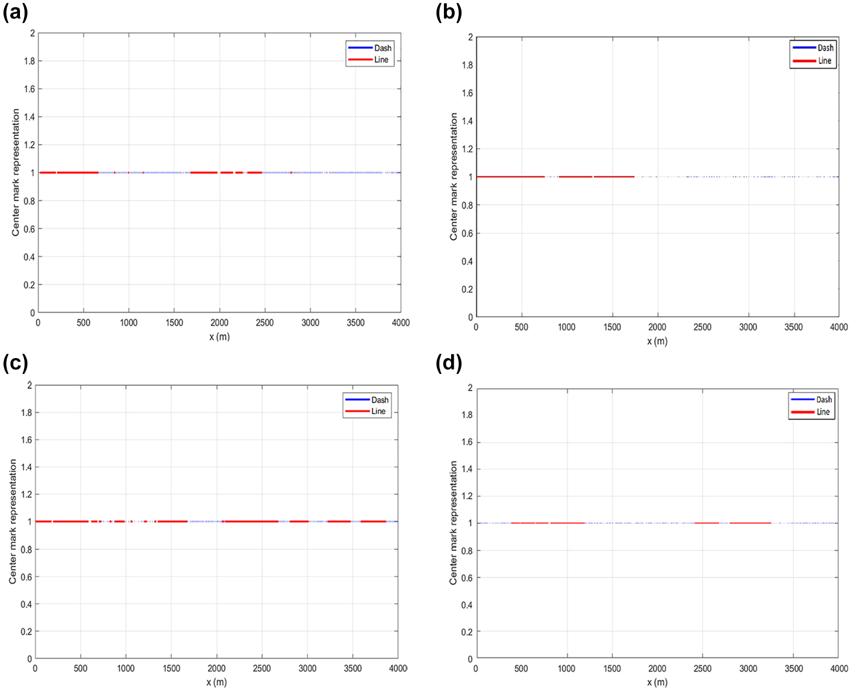
Extracted lane marking for the tested segments: (a) segment 1; (b) segment 2; (c) segment 3; and (d) segment 4.

ASD Assessment and PSD Evaluation along Test Segments (Stages 2 to 5)

Following the extraction of lane marking and the identification of passing and no-passing regions, the ASD for passing was calculated along passing-allowed and passing-prohibited regions. Figure 7 shows the ASD on all segments which is the output from Step 4 of the methodology. The horizontal gray line represents the minimum ASD required for passing (i.e., 740 m or ≈ 2,427.82 ft). In regions where the ASD falls below this line, drivers would not have adequate sight distance to safely perform a passing maneuver. The figures also show the existing lane marking patterns and proposed lane marking lines allocated based on the findings and exact ASD for passing maneuvers.

Figure 7.

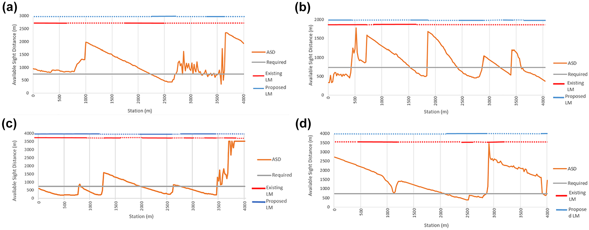
Available sight distance on test segments and existing marking pattern: (a) segment 1; (b) segment 2; (c) segment 3; and (d) segment 4.

For Segment 1, the figure shows that the ASD meets the minimum PSD requirements along the segment, except for regions from Station 2+220 to 2+680 and from Station 3+340 to 3+620. This represents a total distance of 740 m (≈2,427.82 ft) (i.e., 19% of segment length) where the passing maneuver should be prohibited to avoid any safety consequences that could occur as a result of sight distance deficiencies. In comparison, the remainder of the segment (i.e., 3,260 m [≈ 2.03 mi], 81% of segment length) has enough ASD for passing. When checking the pattern of the existing lane marking, the total length of existing passing-permitted zones (i.e., dashed red lines) equals 2,450 m (≈1.52 mi) (i.e., 61% of segment length) and passing-prohibited zones (i.e., solid red lines) equals 1,550 m (≈0.96 mi) (i.e., 39% of segment length). Therefore, the outcome of ASD assessment is used to propose a revised lane marking pattern (i.e., dashed and solid blue lines) that align with the available visible distance for passing and is consistent with the existing conditions of the highway segment.

Using this approach, a passing-prohibited marking line (i.e., solid blue line) is proposed at locations where enough PSD is available, and a passing-allowed marking line (i.e., dashed blue line) is proposed at locations where the ASD is greater than the minimum PSD requirements. This newly proposed marking pattern that agrees with ASD values allows for increasing the total length of passing-allowed zones from 2,450 m (≈1.52 mi) (i.e., 61%) to 3,260 m (≈2.03 mi) (i.e., 81%), enabling more and safer passing opportunities. It also helps prevent unsafe passing maneuvers where, according to the existing marking pattern, passing is currently allowed in regions along which ASD is less than the PSD requirements (e.g., from Station 3+340 to 3+620). Using the same approach, ASD and the existing pattern of lane marking were reviewed for all segments, and new lane marking patterns were proposed based on the findings.

For Segment 2, the proposed lane marking resulted in reducing the total length of passing-permitted regions from 2,445 m (≈1.52 mi) (i.e., 61%) to 2,200 m (≈1.37 mi) (i.e., 55%). This is a result of prohibiting currently permitted passing opportunities along some regions between Station 1+700 and Station 4+000, where the ASD was found to be lower than the PSD requirements. This is demonstrated by the existing (i.e., dotted red) and proposed (i.e., solid blue) marking lines between these station ranges. As shown in the figure, the results of Segment 3 show relative consistency between the pattern and locations of existing and proposed marking lines. This is represented by a total length of 1,400 m (≈0.869 mi) (i.e., 35.0%) of existing passing-allowed zones compared with a total of 1,410 m (≈0.876 mi) (i.e., 35.3%) for the proposed marking lines. The review of Segment 4’s existing conditions and designation of a new marking pattern resulted in increasing the total length of regions along which passing is permitted from 2,520 m (≈1.56 mi) (63%) to 3,050 m (≈1.89 mi) (76%) as shown by the existing and proposed marking patterns. The segment also has locations where passing is proposed to be permitted at regions where it is currently prohibited, although the ASD meets the PSD requirements. Also, there are a few regions where passing is currently allowed, while it must have been prohibited because of sight distance limitations.

The analysis of all segments revealed three general outcomes based on the existing conditions. The first case represents an existing condition (i.e., regions) that meets standard requirements where the ASD meets the minimum PSD requirements and passing is currently allowed. The second case represents a substandard condition that might indicate the presence of safety concerns. In this case, there are locations where passing is currently permitted, but the ASD is lower than the required PSD. The third case is for zones along which passing is currently prohibited, and the ASD is higher than the required PSD, which is a case that represents a non-optimal existing condition. These findings emphasize the presence of imperfections in the existing designation of passing-allowed and passing-prohibited zones. Although highways should have been designed and constructed to meet design requirements, imperfections during construction stages, maintenance operations, practical construction limitations, and budgetary constraints are all potential reasons that could have led to existing conditions that do not meet the standard requirements. This demonstrates the value of using LiDAR data to obtain up-to-date information on highways and emphasizes that the LiDAR point cloud represents data-rich 3-D models of roadways that could be visited virtually and frequently to extract attributes of highway segments and assess existing conditions.

Preliminary Road Safety Review

A high-level road safety review was also conducted to investigate the potential safety implications of regions where passing is currently allowed, but the ASD does not meet the PSD requirements. Historical collisions on the test segments between 2009 and 2014 were mapped onto the ASD. Figure 8 shows the ASD, marking patterns, and plotted crashes using their spatial coordinates. The collisions used in the analysis are crashes that likely occurred as a result of PSD limitations such as sideswipe, run-off-road, and hit-object collisions. Rear-end collisions were excluded because of their high correlation with SSD limitations ( 10 ). A total of 70 collisions occurred in the four segments. As shown in Figure 8, the analysis revealed that 30% of these crashes occurred along regions currently used as passing-allowed zones, although the ASD does not meet the PSD requirements. Although this does not confirm that these collisions occurred because of insufficient sight distance, it demonstrates that sight distance limitations at these regions might have been a contributing factor in collision occurrence. This also identifies these regions as candidates for a more in-depth and detailed safety assessment. These findings demonstrate how serious it could be to permit passing opportunities along regions where ASD is less than PSD requirements. They also emphasize the importance of conducting periodic passing sight distance and safety assessments on highways and demonstrate the value of using LiDAR data for these purposes.

Figure 8.

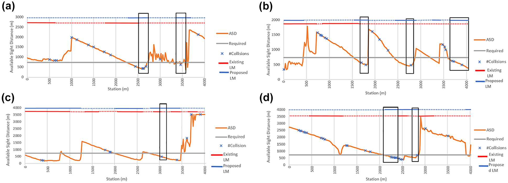
Historical collisions along regions where passing is currently allowed; (a) segment 1; (b) segment 2; (c) segment 3; and (d) segment 4.

The proposed framework demonstrates an automated approach and a tool that can be used for PSD assessment enabling the review of the existing design of highways and the investigation for safety-related issues along highways where sight distance is problematic. Using LiDAR data alleviates the hurdles associated with using traditional approaches such as time consumption, traffic disruption, and the infeasibility of large-scale implementation. It is worth mentioning that one of the core benefits of using LiDAR data is the ability to use the same data set in various applications such as feature extraction, sight distance assessment, cross-section extraction, and roadside evaluation. The value of using LiDAR data lies in using the same data set for multiple purposes. It is worth noting that comparing the costs associated with obtaining and using LiDAR data for one application with using traditional methods is not a feasible comparison ( 27 ). Adopting the use of LiDAR data in asset management could result in considerable cost and time savings. For example, the Savannah-area geographic information system (SAGIS) used LiDAR data to develop contour maps for a drainage improvement project of the Hardin Canal in Georgia ( 39 ). The savings from using LiDAR data were estimated to be $7 million. In a more recent study, Shalkamy et al. ( 12 ) explored the time and cost savings associated with using LiDAR data to detect highway horizontal curves and extract their geometric characteristics along 242 km (≈150.37 mi). Time saving is also a great benefit of using LiDAR datasets. The methodology used in the research by Shalkamy et al. ( 12 , 40 ) has successfully identified 35 horizontal curves in 13 min and 32 s without causing any onsite road closures or safety risks. It was concluded that using LiDAR data in asset management could result in significant time and money savings. In summary, the proposed framework is of great value to both design professionals and transportation agencies and represents a tool that can be used in assessing the compliance of existing roads with design requirements and can be used in investigating safety issues associated with limited sight distance.

Conclusions

This paper introduced a fully automated methodology by which PSD can be computed and evaluated on two-lane two-way highways using remotely sensed LiDAR point clouds. The procedure involves centerline lane marking extraction, passing and no-passing zones definition, and ASD computation along regions where passing is allowed or prohibited. This is followed by assessing passing and no-passing locations based on the ASD and the existing pattern of centerline marking (i.e., whether passing is permitted). The method used was tested on 16 km of LiDAR data collected on highway segments in Alberta, Canada. After assessing the ASD and existing passing and no-passing zones along the test segments, three cases representing the existing conditions were found: first, regions in which the ASD complies with PSD requirements; second, zones along which the ASD is insufficient for passing maneuvers (i.e., substandard regions), based on which passing at these locations should be prohibited; third, locations where passing is currently not allowed, but there is adequate ASD to allow passing maneuvers (i.e., non-optimal existing conditions). Based on these scenarios, a reallocation of passing and no-passing zones was done in which passing is to be prohibited in some areas and allowed in some others.

For the test segments, the reallocation resulted in increasing the total length of passing-permitted zones from 61% to 81% of the segment length for Segment 1 and reducing the total length from 61% to 55% on Segment 2 (i.e., because of the presence of substandard regions). There was no change in the accumulated length of the passing regions on Segment 3 while it was increased from 63% to 76% on the fourth segment. A preliminary safety review was conducted across all test segments along substandard regions. The assessment revealed the presence of PSD-related collisions at these locations, supporting the recommendation to prohibit the currently allowed passing along these regions. A more detailed safety analysis is a potential area for future research. The implemented framework enhances the evaluation of PSD on two-lane highways and represents a tool that is ready to use by transportation agencies to assess and improve the geometry of existing highways. As road design parameters can be feasibly mapped using LiDAR data ( 12 , 41 ), the required changes in design parameters to improve PSD, lane markings, and road safety can be determined on a network level. Future research may also explore developing statistical models that validate the expected relationship between road crashes and PSD limitations. These safety prediction models could relate road collisions to road geometry features including sight distance available for passing maneuvers. As is the case with any research, one limitation of the proposed method is that lane markings need to exist and be captured in the data set to enable successful detection by the proposed method. It is also recommended that roadways be scanned when they are in good condition to have a representative record of the roadway features.