Sage Journals: Discover world-class research

Abstract

In this paper, we address a multi-objective residential waste collection problem with an integrated territory planning and vehicle routing approach. Dividing the problem into territories enables drivers to carry out the same route every week so they get familiar with it and residents put out their bins at the appropriate time. Another benefit is to reduce the computation time for large problems, since the complex characteristics of the involved vehicle routing problem make it otherwise difficult to solve. There are three characteristics that are important for good territory planning: minimum overlap, minimum travel time, and balanced workload. The purpose of this paper is to investigate the influence these three objectives have on each other, since they might be contradictory. Moreover, an Adaptive Large Neighborhood Search (ALNS) algorithm is developed for this specific problem which uses a K-means algorithm to generate the initial solution for territories. The results with the three objectives are shown to be useful for planners seeking to make informed decisions through the trade-off across different solutions with the Pareto frontiers provided. Moreover, the ALNS algorithm is shown to find good quality solutions in a reasonable computational time.

Waste collection is an important topic, since a growing population produces more and more waste and which has a negative impact on the environment ( 1 , 2 ). Four factors that influence the efficiency of waste management are: the amount of waste generated; the number of waste collectors; the amount of effort they put in; and the number of vehicles they run ( 3 ). The high cost of labor and trucks mean that transportation and collection account for the largest proportion of operational costs ( 1 , 4 , 5 , 6 ). Optimizing route planning, therefore, offers scope for the biggest improvement which is why the waste collection problems are usually considered as a specific form of the vehicle routing problem (VRP). There are two aspects that distinguish the waste collection issue from a standard VRP. First, it has several pick-up points, waste collection bins or containers, and one delivery point, a disposal facility. Second, there is the possibility that demand exceeds the capacity of the vehicle, if during the route extra disposal visits are made ( 1 ). Decisions of when to visit a disposal facility and, in the case of several facilities, which one to visit add extra complexity to the decision-making process ( 7 ). As VRP is known to be an NP-hard problem ( 8 , 9 ), our problem also belongs in this category.

In VRP, it is important to represent real-life situations to create solutions which planners and drivers are willing to use, in addition to the aim of reducing costs. First, territories should be both connected and as compact as possible ( 10 ). Compact territories result in smaller travel distances and travel time. When territories are not compact and are unconnected, there are a lot of crossovers between routes. This is not beneficial in practice and models should, therefore, consider minimizing the number of crossovers or overlaps ( 7 ). Operational planners and drivers tend to find plans that look visually attractive (without overlap) easier to accept ( 11 ). Furthermore, solutions with unbalanced workloads will not be accepted by the end users. Considering more balanced solutions brings several advantages such as lower overtime hours, higher employee satisfaction with lower turnover, better customer service, and more flexible use of available capacity ( 12 ). It can also reduce the fluctuation in daily service revenue ( 10 ).

The goal of this paper is to investigate how the three objectives of minimizing travel time, minimizing overlap, and balancing workload influence each other through an integrated territory planning and vehicle routing problem. This makes a clear contribution to the literature for three reasons. (1) There is no study that considers all three objectives at the same time within routing optimization. In most cases the overlap and workload balance are evaluated as post-processing steps but are not considered during the optimization of the routes as objective functions. (2) Territory planning and vehicle routing are modeled in an integrated way. (3) An ALNS algorithm is developed for larger instances of the problem that involve various additional components (e.g., clustering algorithm) to fit it to this multi-objective waste collection problem with territories.

Literature Review

The consideration of waste collection problems has are two main focus points: developing algorithms to solve the optimization problem; and capturing the reality as much as possible using realistic data and constraints ( 2 ). We first provide a review of territory planning that aims to reduce the computation time and then we cover studies that consider overlap and workload balance.

Territory Planning

A way to deal with the complexity of the (waste collection) VRP is to split the total area of customers into territories. The smaller sub-problems are easier to solve and resources can be used several times if the territories can be serviced on different days. Territories can also be beneficial for improving the customer service. Drivers visiting the same set of customers regularly know the area which leads to shorter service and travel times ( 13 ). Besides, they are easier to operate than the whole system together and, if something changes, only part of the global planning needs to be adjusted ( 14 ). Kim et al. ( 7 ) solve a commercial waste collection problem where territories fit the real-life procedure with a fixed schedule. Most literature is based on a two-phase method, in which the clustering and the routing phases are separated ( 8 ). Nevertheless, the clustering solution influences the solution of the routing. A bad clustering assignment might result in higher travel times ( 15 ) and therefore higher operational cost and poor customer service ( 16 ). One of the few examples of researchers not using a two-phase approach is Litvinchev et al. ( 17 ) who solve the pick-up and delivery problem with time windows using territory planning with a mixed integer programming model. Their goal is to minimize the longest zone route to create more balanced territories. They mention problems with computation time when the number of nodes or the number of zones get higher.

Heuristics can provide relatively good solutions for large-scale problems without any optimality guarantee. Among the waste generation papers, local search is the most popular, followed by tabu search ( 6 ). Another often used heuristic is the cluster-first-route-second approach. According to Cordeau et al. ( 8 ), the first type of cluster-first-route-second heuristic used in literature is the sweep algorithm. Gillett and Miller ( 18 ) use this method to solve a vehicle dispatch problem with limited capacity of the vehicles and distance restrictions. Up until their research, most methods could only solve problems with a maximum of 100 nodes. Using territory planning with the sweep algorithm, the problem is split into smaller sub-problems and computation time is reduced. Other examples are the sweep ( 8 ), K-means ( 7 ), and shifting insertion ( 19 ) heuristics.

No Overlap

As mentioned earlier, one important objective in waste collection VRP is route compactness ( 7 ), that is, no overlap, that leads to a route planning with fewer crossovers between the routes. Some literature uses the term visual attractiveness ( 20 ), which refers to compact routes on which no crossovers take place between routes. According to Tang and Miller-Hooks ( 21 ) this is not vital for the implementation of a route plan, but highly desirable and therefore often incorporated in the problem as soft constraints. Some research however argues that solutions are not acceptable if overlap takes place and thus fully eliminates overlap between clusters ( 10 , 19 ).

The importance of fewer crossovers comes mostly from a business point of view. Kim et al. ( 7 ), Tang and Miller-Hooks ( 21 ), and Poot et al. ( 11 ) all state that planners use the visual attractiveness of a solution to determine if the solution is acceptable or not. Kim et al. ( 7 ) even experienced rejections of solutions by planners because of overlapping routes in solutions. The tendency to accept route plans that look visually attractive is because they seem logical to them, even though these solutions might perform worse on other aspects, such as travel time ( 11 , 22 ). Solutions without overlapping routes have clear boundaries and this helps planners to adjust general computer based solutions to specific business needs ( 10 ). Adjustments can be made easily without disrupting other routes in the planning ( 20 , 23 ). This might also be beneficial for real-life disruptions, such as congestion, accidents, or malfunctioning vehicles in the operational phase of waste collection routing. It might seem intuitive that minimizing route time or distance will also lead to clusters in which nodes lie close to each other, which results in less overlap between the clusters. To a certain extent this will probably be the case, but several papers, mention poor results with respect to overlap or visual attractiveness if they are not taken into account explicitly ( 7 , 11 , 24 ). Both Sahoo et al. ( 25 ) and Tang and Miller-Hooks ( 21 ) showed that their algorithm increased the visual attractiveness significantly, when it is explicitly considered, while the increase in travel time was still acceptable.

Workload Balance

From a business point of view, every vehicle serving a territory should perform approximately the same amount of work, for example, number of customers served or travel distance/time. Unbalanced solutions will not be accepted by drivers and route planners ( 7 ) as they result in irregular hours. In addition, there are several advantages to workload balance that are not based on minimizing cost, but can benefit the company ( 12 ). Examples are lower overtime hours, higher employee satisfaction with lower turnover, better customer service, more flexible use of available capacity ( 12 ) and a reduction in the fluctuation in daily service revenue ( 10 ).

There is no single straightforward way to measure workload balance and most research focuses on balancing the tour lengths, however balancing the number of stops, service time, or demand might be more suited for specific problems. Once the measure is selected, a balance method needs to be defined to incorporate it in the objective function. According to Matl et al. ( 12 ) the chosen balance method influences the VRP solution significantly. For example, more complex measures result in a higher number of trade-off solutions. Different balance methods found for the route length are the standard deviation of route length ( 17 ) and the difference between the longest and the shortest route time ( 7 ). For the number of stops, the sum of deviations of the average number of customers in each cluster is used by Cao and Glover ( 10 ). Li et al. ( 19 ) minimize the standard deviation of the number of nodes in a cluster if the demand of all customers is the same or does not matter, otherwise they minimize the standard deviation of the total demands within a cluster. Lum et al. ( 23 ) combine the number of nodes and the travel distance to achieve a balanced route.

The literature also differs in the way the workload balance is evaluated. In most cases it is evaluated after the final solution is created or it is evaluated at improvement steps ( 7 ). Only in a few cases is the measure of the workload balance incorporated into the routing optimization ( 17 ).

Problem Description

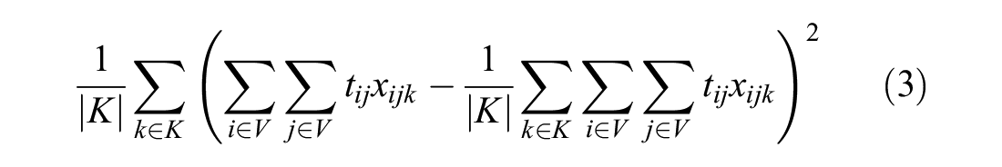
In this research, multiple objectives are incorporated within routing optimization to generate solutions that provide real-life applicability. One of them is the minimization of overlaps between territories to obtain solutions that are compact and visually attractive. The second is the workload balance to generate routes that lead to similar workload across drivers. Finally, a company always tries to minimize cost and it is necessary to find optimal routes through territories, which is incorporated as the third objective through total travel time. The workload balance is measured as the variance of the route travel times in minutes. The overlap value is measured by the sum of the distance between all nodes assigned to the same route.

Since the above-mentioned three objectives influence each other and may be contradictory, there will not be an optimal solution that provides the minimum possible value for all of them at the same time. We, therefore, work with the Pareto frontier which consists of so called non-dominated solutions. According to Ombuki-Berman et al. ( 26 ), a solution vector $u = [x_{1}, x_{2}, \dots, x_{n}]$ is said to dominate another vector $v = [y_{1}, y_{2}, \dots, y_{n}]$ if and only if:

\forall i \in [1, \dots n] : u_{i} \leq v_{i} and \exists i \in [1, \dots, n] : u_{i} < v_{i} .

In this research, such a solution vector u would look like $[t_{u}, o_{u}, w_{u}]$ , in which $t_{u}$ represents the travel time, $o_{u}$ the overlap and $w_{u}$ the workload balance value. This results in solutions in which one of the objectives might decrease, while the others increase. For example, a perfectly balanced route might result in a lot of overlap or higher travel times, to create a solution in which the travel times of all routes are equal.

The vehicle fleet in this paper is considered to be homogeneous, that is, all vehicles have the same maximum load capacity and maximum vehicle routing time. If the vehicle reaches its load capacity, it has to visit a disposal facility. Besides, the number of vehicles is not known upfront. This means several vehicles have to be chosen before the solution method starts. This is needed to determine the number of territories. Vehicles have to start and end at a depot and before a vehicle returns to the depot, it has to visit a disposal facility to arrive empty at the depot. Finally, all nodes should be visited by exactly one vehicle and the demand should be served.

Mathematical Model

We formulate the residential waste collection VRP as a Mixed Integer Quadratic Programming Problem over a network $G = (V, A)$ , where V is the set of nodes and A is the set of arcs. The set V includes the depot (0), the residential stops ( N), and the disposal facilities ( F), that is, $V = {0} \cup N \cup M$ . The travel time between node i and j is given by $t_{ij}$ . A demand $d_{i}$ is associated with customer $i \in N$ . Since a vehicle can visit a node only once, but in reality a disposal facility could be visited multiple times by the same vehicle, the nodes that represent disposal facilities are duplicated. The number of duplicated disposal facility nodes is equal to $⌈ \frac{total demand}{vehicle capacity} ⌉ - 1$ . The set F consists of the original disposal facility nodes and their duplicates. The set of vehicles is represented by K. The binary variable $x_{ijk}$ tracks the route of vehicle k and is equal to 1 if vehicle k travels from stop i to stop j and 0 otherwise. The assignment of a node i to a vehicle k is represented by $z_{ik}$ , which is equal to 1 if vehicle k serves customer i and 0 otherwise. The variable $Q_{ik}$ represents the load of vehicle k at node i. To make sure there are no sub-tours for any vehicle k, the variable $u_{ik}$ is introduced. Last, variable $b_{ijk}$ is used to minimize the distance between every two nodes assigned to vehicle k. It is equal to 1 if both node i and j are assigned to vehicle k and 0 in all other cases. The vehicles have restrictions related to capacity C and operation time O.

The objective function (4) minimizes one of the three objectives, total travel time (1), overlap (2), and workload balance (3):

\sum_{k \in K} \sum_{i \in V} \sum_{j \in V} t_{ij} * x_{ijk}

(1)

\sum_{i \in N} \sum_{j = i + 1}^{N} \sum_{k \in K} t_{ij} * b_{ijk}

(2)

\frac{1}{| K |} \sum_{k \in K} {(\sum_{i \in V} \sum_{j \in V} t_{ij} x_{ijk} - \frac{1}{| K |} \sum_{k \in K} \sum_{i \in V} \sum_{j \in V} t_{ij} x_{ijk})}^{2}

(3)

To enable the model to minimize one of the three objectives and limit the other two with an upper bounds of $ε_{1}$ and $ε_{2}$ , constraints (5) and (6) are introduced. The objective chosen to be minimized is denoted by $Objective a$ and the other two objectives that are bounded, are given as $Objective b$ and $Objective c$ .

min Objective a

(4)

s . t . Objective b \leq ε_{1}

(5)

Objective c \leq ε_{2}

(6)

For minimizing the overlap, it is necessary that the model can calculate the distance between nodes assigned to the same vehicle. Constraints (7)–(9) together make sure this is possible.

b_{ijk} \leq z_{ik} \forall k \in K, i \in N, j \in {i + 1, \dots, N}

(7)

b_{ijk} \leq z_{jk} \forall k \in K, i \in N, j \in {i + 1, \dots, N}

(8)

z_{ik} + z_{jk} = b_{ijk} + 1 \forall k \in K, i \in N, j \in {i + 1, \dots, N}

(9)

Constraints (10) and (11) are assignment constraints. They ascertain whether a customer is visited exactly once by one of the vehicles and all vehicles start from the depot, respectively.

\sum_{k \in K} z_{ik} = 1 \forall i \in N

(10)

\sum_{k \in K} z_{0 k} = | K |

(11)

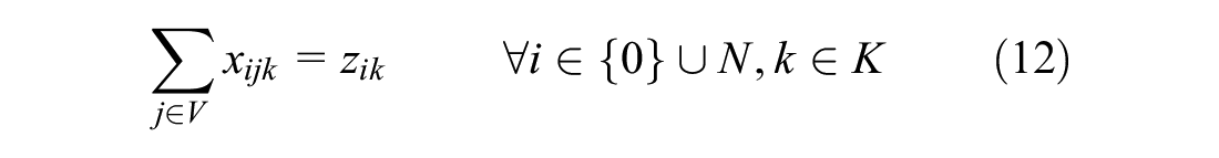
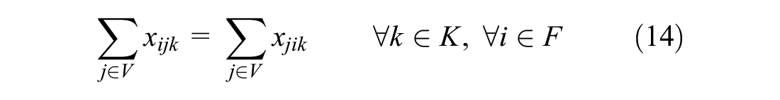
Flow conservation is taken care of by constraints (12)–(14). Combined with constraint (11) it is assured that the routes start and end at the depot for all vehicles.

\sum_{j \in V} x_{ijk} = z_{ik} \forall i \in {0} \cup N, k \in K

(12)

\sum_{i \in V} x_{ijk} = z_{jk} \forall j \in {0} \cup N, k \in K

(13)

\sum_{j \in V} x_{ijk} = \sum_{j \in V} x_{jik} \forall k \in K, \forall i \in F

(14)

Constraint (15) prohibits the load of a vehicle to exceed its capacity and when a vehicle visits a disposal facility to empty its content Constraint (16) sets the load back to zero. Constraints (17) and (18) keep track of the load. If a vehicle drives from a resident to a disposal facility, the disposal facility must be assigned to the vehicle to keep track of the routes, so Constraint (19) takes care of this. Constraint (20) ensures the maximum total vehicle routing time is not exceeded.

Q_{ik} \leq C \forall k \in K, i \in N

(15)

Q_{ik} = 0 \forall k \in K, i \in {0} \cup F

(16)

Q_{ik} + d_{j} \leq Q_{jk} + (1 - x_{ijk}) * C \forall k \in K, i \in V, j \in N

(17)

Q_{jk} \leq Q_{ik} + d_{j} + (1 - x_{ijk}) * C \forall k \in K, i \in V, j \in N

(18)

\sum_{i \in N} x_{ijk} = z_{jk} \forall k \in K, j \in F

(19)

\sum_{i \in V} \sum_{j \in V} t_{ij} * x_{ijk} \leq O \forall k \in K

(20)

Constraints (21) and (22) eliminate sub-tours. Furthermore, a vehicle must be empty when it arrives at the depot which is ensured by Constraint (23) by avoiding a depot visit directly after a customer visit. In addition, it does not make sense to go to a disposal facility without a load, so Constraint (24) makes sure routes do not visit two disposal facilities consecutively and Constraint (25) makes sure vehicles do not go directly from the depot to a disposal facility.

1 \leq u_{i} \leq | V | + 1 \forall i \in N + F

(21)

u_{jk} \geq u_{ik} - (| V | + 1) * (1 - x_{ijk}) + 1 \forall i, j \in F + N

(22)

x_{i 0 k} = 0 \forall k \in K, i \in N

(23)

x_{ijk} = 0 \forall k \in K, i, j \in F

(24)

x_{0 jk} = 0 \forall k \in K, j \in F

(25)

Finally, Constraints (26) and (27) define x, z, and b as binary variables, Constraint (28) enforces non-negativity for the load and Constraint (29) defines the variables for sub-tour elimination.

x_{ijk}, z_{ik} \in {0, 1} \forall k \in K, i, j \in V

(26)

b_{ijk} \in {0, 1} \forall k \in K, i \in N, j \in {i + 1, \dots, N}

(27)

Q_{ik} \geq 0 \forall k \in K, i \in V

(28)

u_{ik} \in ℛ \forall i \in N + F, k \in K

(29)

Solution Algorithm

We develop an ALNS heuristic to deal with the solution of the problem for large size instances. ALNS takes an initial solution and adjusts it in every iteration by first destroying part of the solution and then repairing it. For the type of problems we have, this means first removing some nodes from a territory and afterwards inserting them in the remaining territories. To make sure solutions are feasible, capacity constraints of the vehicle and maximum routing times are taken into account when re-inserting the nodes. An overview of the full ALNS heuristic is displayed in Figure 1.

Figure 1.

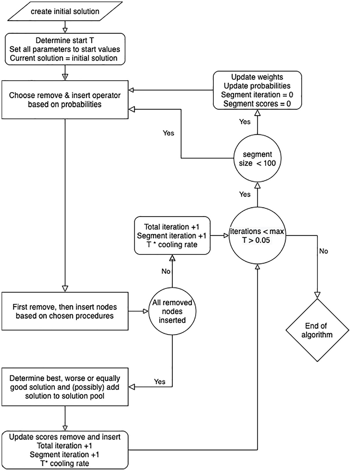
ALNS procedure.

Finding an Initial Solution

A K-means algorithm is used for the initial solution (Algorithm 1) to generate the territories. First, the number of clusters (NC) to be created is determined based on the demand and the capacity:

NC = ⌈ \frac{total demand}{vehicle capacity} ⌉ .

Algorithm 1 K-means
1: NC ← number of clusters to create
2: Choose seed nodes for NC clusters from all nodes
3: for all other nodes n do
4: closest _ seed _ n ← assign node n to closest seed node
5: end for
6: For all clusters calculate center of gravity
7: center _ node _ c ← closest node to center of gravity of cluster c
8: while non of the three stopping criteria reached do
9: for all nodes n do
10: closest _ seed _ n ← reassign n to closest center _ node _ c
11: end for
12: calculate new center _ node _ c after reassigning nodes for all clusters c
13: end while

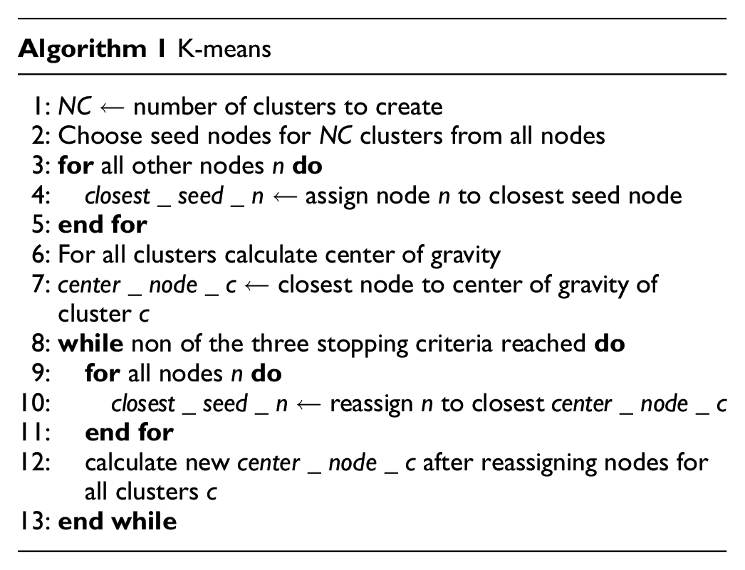
Then NC random customer nodes are chosen as seed nodes for the clusters. The next step is to assign all other nodes to the cluster of the seed node that is closest to them. When all nodes are assigned, the new center of gravity of the cluster is calculated. The node nearest to the center of gravity is assigned the new cluster seed node. Afterwards, for all nodes it is determined whether the new cluster seed is still the nearest to them. If this holds for all nodes, the algorithm stops. If not, it reassigns all nodes to their nearest seed node and the iterations start again. There are three situations in which the algorithm stops: (i) when all nodes are assigned to the cluster with the seed node closest to them; (ii) when the algorithm keeps on iterating infinitely with repeating solutions; and (iii) when 100 iterations is reached.

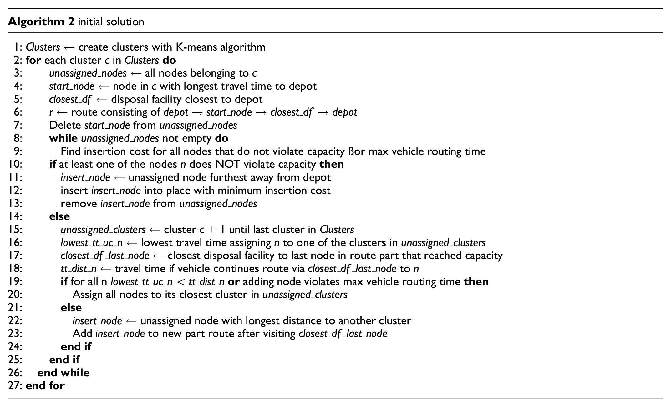
In the K-means algorithm, the capacity of the vehicles and the maximum routing time is not considered yet. So after creating these clusters, routes are created for each cluster as given by Algorithm 2. If the routes created cannot accommodate all the nodes to be visited, the algorithm adds one extra vehicle to the problem and a new solution is created with the K-means procedure.

Algorithm 2 initial solution
1: Clusters ← create clusters with K-means algorithm
2: for each cluster c in Clusters do
3: $unassigned_nodes$ ← all nodes belonging to c
4: $start_node$ ← node in c with longest travel time to depot
5: $closest_df$ ← disposal facility closest to depot
6: r ← route consisting of $depot \to start_node \to closest_df \to depot$
7: Delete $start_node$ from $unassigned_nodes$
8: while $unassigned_nodes$ not empty do
9: Find insertion cost for all nodes that do not violate capacity ßor max vehicle routing time
10: if at least one of the nodes n does NOT violate capacity then
11: $insert_node$ ← unassigned node furthest away from depot
12: insert $insert_node$ into place with minimum insertion cost
13: remove $insert_node$ from $unassigned_nodes$
14: else
15: $unassigned_clusters$ ← cluster $c + 1$ until last cluster in Clusters
16: $lowest_tt_uc_n$ ← lowest travel time assigning n to one of the clusters in $unassigned_clusters$
17: $closest_df_last_node$ ← closest disposal facility to last node in route part that reached capacity
18: $tt_dist_n$ ← travel time if vehicle continues route via $closest_df_last_node$ to n
19: if for all n $lowest_tt_uc_n$ < $tt_dist_n$ or adding node violates max vehicle routing time then
20: Assign all nodes to its closest cluster in $unassigned_clusters$
21: else
22: $insert_node$ ← unassigned node with longest distance to another cluster
23: Add $insert_node$ to new part route after visiting $closest_df_last_node$
24: end if
25: end if
26: end while
27: end for

Solution Pool and Acceptance Criteria

All non-dominated solutions are saved in a solution pool, SP. A solution s is added to SP if it is accepted by the algorithm based on the following criteria:

The solution s is the best solution that is found, that is, $s_{i} < u_{i} \forall u \in SP, i \in [1, 2, 3]$ ;

The solution s is not dominated by any of the solutions $u \in SP$ ;

The solution s is dominated by at least one of the solutions in SP, but is accepted based on the acceptance probability of the simulated annealing algorithm.

In the first case, the solution pool created so far is deleted, as the new found solution dominates all. In the second and third cases, the solution is added to the existing pool. The third case is included to avoid getting stuck in a local optimum based on the simulated annealing idea where a large temperature value T is selected initially and with every iteration the temperature is cooled down by a cooling rate, with $0 < coolingrate < 1$ . The acceptance probability of a worse solution with value $v_{worse}$ is given by:

P (rd < \exp (\frac{v_{current} - v_{worse}}{T}))

where $v_{current}$ is the value of the last added solution and rd is a random number between 0 and 1. As T decreases, the acceptance probability decreases. Since we have three individual objective function values, they have to be combined to determine if a worse solution has to be accepted.

Removal Operators

For neighborhood search, the first step is to remove part of the solution. The number of nodes removed and the rule by which they are removed vary per iteration. If nodes are removed from a route, the demand and length of the route are changed accordingly. Since we consider three objectives, there are different variations of the same removal operator for every objective.

For random and worst removal, a number q is chosen as the number of nodes to be removed. There are three different ranges from which to choose the value q: small, medium, and large. In the small case, the value of q can vary between 1% and 30% of the total number of customer nodes. This range is 31% to 70% for the medium case and 71% to 100% for the large case.

Random Removal

The random removal operator can be of three different types, namely removing nodes, a route, or a cluster. When removing nodes, the algorithm chooses q customer nodes from the total set of customer nodes at random and removes these nodes from their routes. The number that is chosen for q lies in one of the three ranges mentioned above. With route removal, the algorithm picks one of the routes at random and deletes all customer nodes in that route. With cluster removal, a random number is chosen, nc, between the number of routes and the number of nodes, which represent the number of clusters. With Kruskal’s minimum spanning tree algorithm ( 27 ), clusters are created of nodes that lie closest to each other. Note that these clusters are not considered to be territories, so they could be assigned to different routes. The algorithm is stopped when the customer nodes belong to nc groups. One of these nc groups is randomly chosen and all nodes belonging to this chosen cluster are removed.

Worst Node

The worst node removal chooses q nodes to be removed, where q can lie in one of the three ranges mentioned above. It uses the objective function to determine which customer nodes are the worst q nodes. Since, the goal of this research is to find solutions that can be minimized for all three objectives, the worst node is the one that adds the most cost to the solution, in which the cost means something different for every single objective. Therefore, three different worst node removal heuristics are created, one for each of the objectives.

Worst Route

The worst route is the route that increases the cost the most (depending on the objective function) all nodes in this route are removed.

Worst Cluster

For each cluster created by Kruskal’s algorithm, the savings are calculated if it is removed and the one with the highest savings according to one of the three objectives is chosen to be actually removed.

Remove All Routes Worse Than Random Chosen Route with Respect to Travel Time

This removal procedure is used for improving the travel time. First, it randomly chooses a route from the set of all routes. The length of the chosen route is compared with all the other routes. The routes that have a longer travel time than the chosen route will be removed. If the chosen one is the longest then it is removed (equivalent to the worst route removal operator with respect to travel time).

Radius Based Removal

This removal operator focuses on improving the overlap. First, a radius is randomly chosen between 1 and 20 and a seed node is randomly chosen from the set of customer nodes to create a circle, with the seed node as its center. The algorithm searches for nodes that lie within the circle, but do not belong to the same route as the seed node. If it finds nodes that meet this criterion, it removes them, otherwise it does not remove any of the nodes.

Remove All Routes Worse Than Random Chosen Route with Respect to Workload

To get a better solution for workload balance, this operator chooses a random route and will delete all routes that differ more than p % in length, where p can vary in the same three categories as for the removal of the nodes, mentioned at the beginning of the section. If there are no other routes as such, the randomly chosen route will be removed.

Insertion Operators

The second step of neighborhood search is to insert the elements that were removed into the solution. Just as with the removal operators, different methods are used and there are variations of each method considering the three objectives. It is important to bear in mind that a node cannot be inserted between a disposal facility and a depot. Also, feasibility with respect to the capacity of a vehicle and the maximum routing time needs to be maintained.

Greedy Insertion

This operator iterates over a list of nodes that have to be inserted. It picks the first node in the list and finds the “best” place to insert the node in one of the routes. Which place is the best, depends on the objective considered. It does not consider other nodes when finding the best insertion place for this node. If for at least one of the nodes no feasible insertion place can be found, either because of the maximum routing time or the capacity of the vehicle, the solution is rejected.

Best Insertion

The best insert operator also looks for the best insertion place, but in this case it considers all the nodes at the same time. The algorithm first finds the best insertion place for each node and chooses the overall best value from the best values of all the nodes. It inserts this node and the whole procedure is then repeated until there are no nodes left to insert. If at least one of the nodes cannot be inserted because of limited capacity or route time, the whole solution is rejected.

Regret Insertion: Next Best

The regret insertion operator is based on the idea that it is beneficial not just to consider the best insertion place at the moment, but also the consequences thereafter. If there is one node for which the difference between its best and second best insertion places is very high, it could be better to insert this node first, because it might give issues with capacity constraints or unsatisfactory solutions later on. The regret here is defined as the difference between the best and second best route. In one iteration the regret of every node is calculated and the node with the largest regret is chosen to be inserted first. This procedure is repeated until there are no nodes left to insert. If a node cannot be inserted in one of the routes, it gets a very high penalty for this route. If no insertion is possible at all for at least one of the nodes, the solution is rejected.

Regret Insertion: Summed

The difference with the previous operator is that the regret is defined as the sum of the differences of all routes from the best route. The node with the highest regret is chosen to be inserted first. If at least one of the nodes cannot be inserted in any of the routes, the solution is rejected.

Adaptive Weights

For each iteration a removal and an insertion operator are chosen and the probability to choose one of them is based on a weight $w_{i}$ . The probability $p_{j}$ to choose operator j with weight $w_{j}$ is determined by: $\frac{w_{j}}{\sum_{i} w_{i}}$ . When the algorithm starts, the weights are the same across the operators. The algorithmic procedure is split into so called segments and after each segment sg the weights are adjusted and the probabilities are updated. We use the definition by Ropke and Pisinger ( 28 ), so that one segment represents 100 iterations of the ALNS algorithm.

The adjustment of the weight is based on how well the algorithm performs in finding solutions represented by a score. At the beginning of each segment (100 iterations), the scores for all the insertion and removal operators are set to zero. With each new solution, the score is increased by one of the following: $σ_{1}$ when the new solution is better than all the solutions so far; $σ_{2}$ when it is better than the current solution; $σ_{3}$ when it is worse than the current but still accepted; and finally 0 when it is rejected. It is not clear whether the removal or the insertion operator leads to the new solution, so their scores are both adjusted by the same value. Scores add up during the iterations in a given segment sg for each operator i and for the next segment $sg + 1$ it is updated as follows:

w_{j}^{sg + 1} = (1 - r) w_{j}^{sg} + r π_{j}^{sg}

where r is a value between 0 and 1 and $π_{j}^{sg}$ is defined as

π_{j}^{sg} = \frac{score of operator j after sg}{number of times operator j chosen in sg} .

The parameter r is used to control how much the change in weight depends on how well the operator performed in the last segment. If r is 1, the weight completely depends on the performance in the last segment and otherwise the weights do not change.

Results

To evaluate the impact of optimizing travel costs, overlap, and workload balance, several experiments are conducted. First, the exact approach is analyzed based on Solomon’s instances and then ALNS is tested compared with the exact approach and finally a real-life case is presented. The Mixed Integer Quadratic Programming Problem and ALNS were implemented in Python and the exact solution obtained by Gurobi optimizer (version 8.1.1).

Solomon’s Instances – Exact Solution

Solomon’s instances R101 and C101 with 25 nodes are used for the experiments. One depot and two disposal facilities are considered. The vehicles have a maximum capacity of 200 and a maximum vehicle routing time of 700 min. Based on the combination of the demand and vehicle capacity, we need at least two vehicles and we also tested with three vehicles to see the impact on the three objectives and the territory solutions. The O-D matrix for Solomon’s instances are created based on the Euclidean distance measure and a constant speed is assumed to represent travel time.

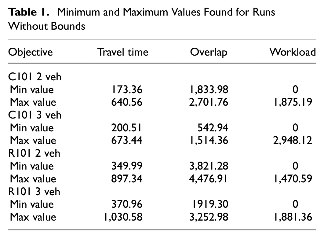
For all the experiments, a time limit of two central processing unit (CPU) hours is used. First, every objective was optimized without any bound on the other two objectives to determine the ranges to be considered. The minimum and maximum values found for these runs in both the C101 and R101 cases with two or three vehicles are displayed in Table 1. The bounds are then chosen in between the maximum and minimum values for each objective. Every run with varying bounds results in only one solution. When combining all the results, the Pareto frontier can be derived.

Table 1.

Minimum and Maximum Values Found for Runs Without Bounds

Objective	Travel time	Overlap	Workload
C101 2 veh
Min value	173.36	1,833.98	0
Max value	640.56	2,701.76	1,875.19
C101 3 veh
Min value	200.51	542.94	0
Max value	673.44	1,514.36	2,948.12
R101 2 veh
Min value	349.99	3,821.28	0
Max value	897.34	4,476.91	1,470.59
R101 3 veh
Min value	370.96	1919.30	0
Max value	1,030.58	3,252.98	1,881.36

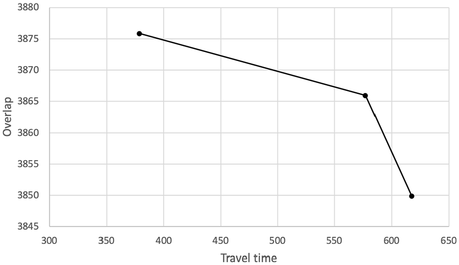
The results confirm that the optimal values for all three objectives were not found at the same time in one of the results, showing their contradictory nature. Furthermore, tighter bounds on the other two objectives can still give the minimum value for overlap or workload balance or at least a value that is fairly close to the optimal value. For the overlap this is displayed in Figure 2, where several solutions exist with the optimal value, 1,919.30, and varying values for the workload. For the two higher values, 1,996.90 and 2,050.51, there is still no overlap, but the territories in these solutions are less compact. This shows that lower values for both workload balance and travel time can be achieved if the user is willing to give up some compactness. For the workload balance this can be seen in Figure 3 and from the first two values in Figure 4. For these solutions, a value of (approximately) zero is found, with varying travel time and overlap values. In some cases, the optimal solution was not found within 2 h, which resulted in the points in Figure 4 that do not have a workload balance value of zero.

Figure 2.

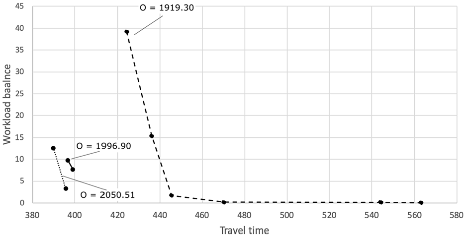
Minimize overlap (three different overlap values): travel time versus workload balance.

Figure 3.

Minimize workload balance (all values optimal): travel time versus overlap.

Figure 4.

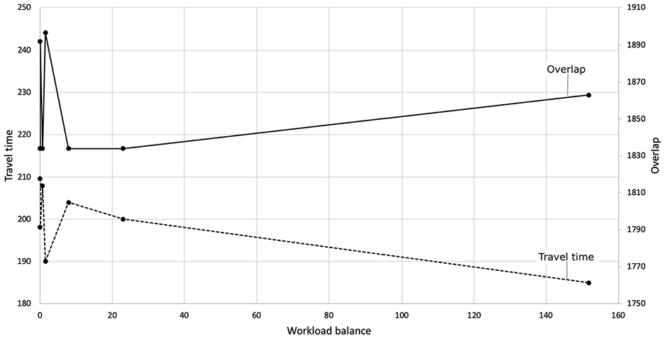
Minimize workload balance: workload balance versus travel time and overlap.

For the travel time, the optimal value can only be found when the bounds of the overlap and workload balance are extremely high as shown in Figure 5, where the travel time increases with lowering at least one of the two values. The reason behind this is that the same territories can be created with many different routes. These different routes can still result in the optimal overlap value, as long as the territories contain the points that result in the lowest overlap value. The same holds for the variance of routes, several different routes could still result in the same variance of the route length. However, only few routes with the exact same travel time can be reached. If either the workload balance or the overlap bound is tightened, exactly the same routes might not be possible and therefore the total travel time would slightly increase.

Figure 5.

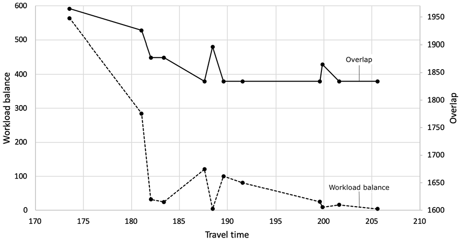
Minimize travel time: travel time versus overlap and workload balance.

Overlap and workload balance seem the two least contradictory variables. The optimal values for the two objectives are found together in all four cases when the overlap measure is minimized. Without any restriction on travel time, it is possible to find routes that have equally long travel times, given a fixed set of nodes. This set of nodes can be the nodes that belong to the territories that give the optimal overlap value. Travel time and overlap seem to be partially contradictory. The lowest overlap value does result in higher travel time values. Increasing the overlap value, allows lower travel time values, which is clearly displayed in Figures 3 and 5. At some point the travel time value is high enough and the solution also gives the optimal overlap value and increasing the travel time more would not decrease the overlap further. This can be seen in Figure 5, where the lowest value of the overlap, 1,833.98, is already found at a travel time of 187.61. This might be explained by the fact that the territories creating the optimal overlap value, might add extra travel time to the routes. Overall, if travel time is more important than the overlap, the overlap value can be kept higher and this does not necessarily impose a problem for the overlap, as long as the number of nodes within more than one convex hull is still zero. In these situations the nodes within a territory may lie further apart (less compact), but do not overlap.

Solomon’s Instances – ALNS

To see if ALNS is suited to finding the different solutions on the Pareto frontier, it is compared with the exact approach based on Solomon’s instances. The parameters used for ALNS are mostly taken from Ropke and Pisinger ( 28 ). The maximum number of iterations is 20,000 (stopping criteria) and the segment size is 100 iterations. The threshold value for the temperature T is set as 0.05 (stopping criterion) and the cooling rate is 0.99975. $σ_{1}$ , $σ_{2}$ , and $σ_{3}$ are set as 33, 9, and 13, respectively. For each of the experiments, ALNS is repeated five times because of its random nature.

Overall, the ALNS algorithm seems to find similar results as the exact approach. When focusing on one of the objectives, it finds the minimum value provided by the exact approach in at least one of the replications. In most cases, it is even able to find lower travel time values in combination with either overlap or workload balance. However, combinations of both low overlap and low workload balance values do not seem to be found by the algorithm. The reason is that ALNS finds the best insertion place per route in the added travel time by our design. Thereafter, it determines the best insertion place for the overlap and workload balance objective. So, even when the algorithm tries to find better values for the overlap or workload balance, it will still have a considerably low travel time. From the exact solution analysis it became clear that a solution with both low overlap and workload balance value has a high travel time value. As the largest travel times are not found, the combination of low or even optimal overlap and workload balance values are not found by the algorithm.

To illustrate this comparison to the exact solution method better, the Pareto frontier of travel time against workload balance is shown in Figure 6. The blue line represents the results of the exact solution method, in which the travel time was optimized with varying upper bounds for the overlap and workload balance values. Since the optimal solution was not always found within the time limit of 2 h, the best bound available is represented by the green line. The orange line gives the solutions on the Pareto frontier found by the ALNS algorithm. As can be seen, ALNS follows the line of the exact solution and it sometimes finds lower combined values for travel time and workload balance than the values found by the exact approach (within the time limit).

Figure 6.

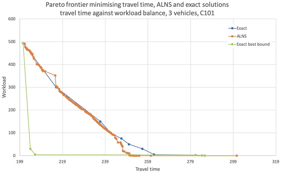
Minimize travel time: travel time versus workload balance – ALNS and exact solutions.

When we look at the computation time, ALNS is significantly faster than the exact solver which needs on average 56 min to find just one solution. On the other hand, ALNS performs 20,000 iterations in 2.4% of this time.

Real-Life Case Study

To evaluate the performance of ALNS for a real-life situation, a case study from the AMCS company¹ was taken and compared with the results from their actual planning model. The case considered is part of the Stonegate neighborhood in the area of Tampa and consists of 120 nodes as depicted in Figure 7. This was the largest case of the cases provided by AMCS that the ALNS heuristic was able to solve. Seven vehicles were used in this case study. The travel times for this network are actual travel times based on the available data rather than Euclidean distances.

Figure 7.

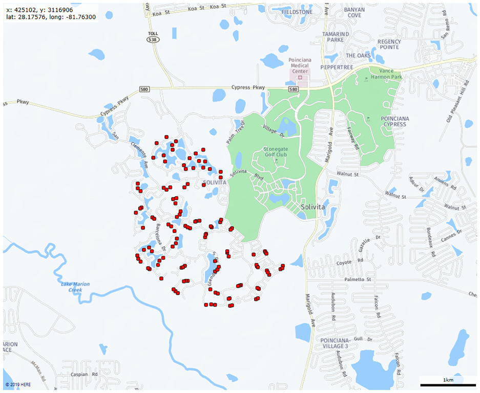
Map of Stonegate with 120 residential waste collection points.

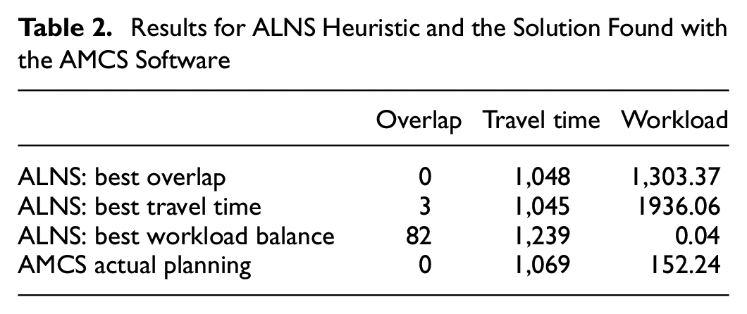
The values of the optimal solution for each of the three objectives and the corresponding values of the other two objectives created by the ALNS algorithm are displayed in Table 2. For the overlap objective, the value for number of nodes in more than one convex hull is chosen as the measure since this compares directly to the results from AMCS. At the bottom row, the values for the solution created by the AMCS planning software are displayed. This AMCS solution is displayed in Figure 8 where Figure 8b is the zoomed-in version to better depict the actual territories and routes. It is seen that there is no overlap between territories in the AMCS solution, while the total route time is 1,069 min with a 152.24 min of variance (representing workload balance) across the seven routes corresponding to seven vehicles.

Table 2.

Results for ALNS Heuristic and the Solution Found with the AMCS Software

	Overlap	Travel time	Workload
ALNS: best overlap	0	1,048	1,303.37
ALNS: best travel time	3	1,045	1936.06
ALNS: best workload balance	82	1,239	0.04
AMCS actual planning	0	1,069	152.24

Figure 8.

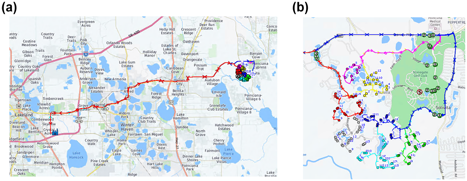
AMCS solution obtained by the AMCS planning software: (a) whole network; and (b) zoomed in.

From the results it is concluded that ALNS is able to find low values for each of the three objectives, that are better than the actual AMCS values, when they are optimized individually. Nevertheless, it is hard to combine these low values in one solution. For the overlap and travel time values, a reasonable combination for both values can be found, since the travel time value in the optimal overlap solution is only three min higher than the best travel time value. However, combining workload balance with one of the two other objectives seems to be difficult. According to the solution of the AMCS software, it can be deduced that is not a problem to have a somewhat higher travel time or workload balance to get zero overlap. The travel time and variance values are respectively 24 min and 152.2 min higher than the optimal solutions found by the ALNS algorithm. However, if an intermediate solution of ALNS for travel time and workload balance is taken, this does not result in zero overlap. For example, the solution with a workload balance value of 133.85 and a travel time of 1,089 min, still has 14 overlapping nodes. This suggests the ALNS algorithm is open for further improvements.

Conclusions

This research develops an integrated territory planning and vehicle routing approach for a real-life waste collection problem. In order for a territory planning to be accepted by planners and drivers, literature and the real-life experience of the AMCS company suggest that balancing the workload and minimizing overlap are important factors. However, these factors might run counter to another important objective of travel cost minimization which is represented by travel time in this paper. An analysis of these three objectives has been performed and depicted through Pareto frontiers. These results provide insights to planners on the trade-off across these objectives. For example, first creating territories to minimize the overlap has a negative effect on travel time minimization and workload balance. Similarly, decision makers can consider these trade-offs to adjust the solution toward desired directions. For example, good values for both travel time versus overlap and workload balance can be achieved if the user is willing to give up some compactness.

An ALNS heuristic has been developed to solve larger problems and validated with a real-life case study showing its potential use by waste collection companies to look at the different possible solutions when making decisions. This is a more informed decision as the planner knows what the trade-offs across the three objectives are. The ALNS heuristic has to be developed further to solve even larger cases and to find combinations of both low workload balance and overlap values.

It is important to investigate the real-life importance of the three objectives to conclude which of the solutions on the Pareto frontier should be implemented. Furthermore, it might be interesting to see if our conclusions hold in a variant of the model presented that for example incorporates multiple depots or uses a periodic schedule, which are cases that could both happen in real-life. Similarly, the impact of the density of the network in waste collection points and the roads could be investigated further to generalize the conclusions even more. Moreover, the problem we consider here is a deterministic and static problem. Future research toward dynamic and stochastic waste collection problems is very interesting with the increasing use of smart containers that provide real-time information on the waste levels.

Footnotes

Acknowledgements

We are grateful for the support of AMCS B.V. by providing the case study data, especially Jelmer Brandt for his valuable contributions.

Author Contributions

The authors confirm contribution to the paper as follows: study conception and design: S. Hurkmans, B. Atasoy, M.Y. Maknoon, R.R. Negenborn; data collection: S. Hurkmans; analysis and interpretation of results: S. Hurkmans, B. Atasoy, M.Y. Maknoon; draft manuscript preparation: S. Hurkmans, B. Atasoy. All authors reviewed the results and approved the final version of the manuscript.

Declaration of Conflicting Interests

The author(s) declared no potential conflicts of interest with respect to the research, authorship, and/or publication of this article.

Funding

The author(s) received no financial support for the research, authorship, and/or publication of this article.

ORCID iDs

Sarah Hurkmans

M. Yousef Maknoon

Rudy R. Negenborn

Bilge Atasoy

Notes

References

Han

Cueto

E. P.

Waste Collection Vehicle Routing Problem: Literature Review. PROMET-Trafﬁc & Transportation, Vol. 27, No. 4, 2015, pp. 345–358.

Idrus

Ku-Mahamud

K. R.

Benjamin

A. M.

Waste Collection Vehicle Routing Problem Benchmark Data sets and Case Studies: A Review. Journal of Theoretical and Applied Information Technology, Vol. 95, No. 5, 2017, pp. 1048–1062.

Das

Bhattacharyya

B. K.

Optimization of Municipal Solid Waste Collection and Transportation Routes. Waste Management, Vol. 43, 2015, pp. 9–18.

Labadie

Prins

Vehicle Routing Nowadays: Compact Review and Emerging Problems. In Production Systems and Supply Chain Management in Emerging Countries: Best Practices ( Mejía

Velasco

eds.), Springer, Berlin, Heidelberg, 2012. https://doi.org/10.1007/978-3-642-26004-9_8

Markov

Varone

Bierlaire

The Waste Collection VRP with Intermediate Facilities, a Heterogeneous Fixed Fleet and a Flexible Assignment of Origin and Destination Depot. Transport and Mobility Laboratory, Ecole Polytechnique Federale de Lausanne, Lausanne, Switzerland, 2015.

Beliën

De Boeck

Van Ackere

Municipal Solid Waste Collection and Management Problems: A Literature Review. Transportation Science, Vol. 48, No. 1, 2012, pp. 78–102.

Kim

B.-I.

Kim

Sahoo

Waste Collection Vehicle Routing Problem with Time Windows. Computers & Operations Research, Vol. 33, No. 12, 2006, pp. 3624–3642.

Cordeau

J.-F.

Laporte

Savelsbergh

M. W.

Vigo

Vehicle Routing. Handbooks in Operations Research and Management Science, Vol. 14, 2007, pp. 367–428.

Braekers

Ramaekers

Van Nieuwenhuyse

The Vehicle Routing Problem: State of the Art Classiﬁcation and Review. Computers & Industrial Engineering, Vol. 99, 2016, pp. 300–313.

10.

Cao

Glover

Creating Balanced and Connected Clusters to Improve Service Delivery Routes in Logistics Planning. Journal of Systems Science and Systems Engineering, Vol. 19, No. 4, 2010, pp. 453–480.

11.

Poot

Kant

Wagelmans

A. P. M.

A Savings Based Method for Real-Life Vehicle Routing Problems. Journal of the Operational Research Society, Vol. 53, No. 1, 2002, pp. 57–68.

12.

Matl

Hartl

R. F.

Vidal

Workload Equity in Vehicle Routing: The Impact of Alternative Workload Resources. Computers & Operations Research, Vol. 110, 2019, pp. 116–129.

13.

Schneider

Stenger

Schwahn

Vigo

Territory-Based Vehicle Routing in the Presence of Time-Window Constraints. Transportation Science, Vol. 49, No. 4, 2014, pp. 732–751.

14.

Teixeira

Antunes

A. P.

de Sousa

J. P.

Recyclable Waste Collection Planning—A Case Study. European Journal of Operational Research, Vol. 158, No. 3, 2004, pp. 543–554.

15.

Giosa

Tansini

Viera

New Assignment Algorithms for the Multi-Depot Vehicle Routing Problem. Journal of the Operational Research Society, Vol. 53, No. 9, 2002, pp. 977–984.

16.

Hadjiconstantinou

Baldacci

A Multi-Depot Period Vehicle Routing Problem Arising in the Utilities Sector. Journal of the Operational Research Society, Vol. 49, No. 12, 1998, pp. 1239–1248.

17.

Litvinchev

Cedillo

Velarde

Integrating Territory Design and Routing Problems. Journal of Computer and Systems Sciences International, Vol. 56, No. 6, 2017, pp. 969–974.

18.

Gillett

B. E.

Miller

L. R.

A Heuristic Algorithm for the Vehicle-Dispatch Problem. Operations Research, Vol. 22, No. 2, 1974, pp. 340–349.

19.

Chen

Cao

Claramunt

An Iterative Two-Step Approach to Area Delineation. In Web and Wireless Geographical Information Systems. W2GIS 2019 ( Kawai

Storandt

Sumiya

eds.). Lecture Notes in Computer Science, Vol. 11474. Springer, Cham. https://doi.org/10.1007/978-3-030-17246-6_1.

20.

Rossit

D. G.

Vigo

Tohmé

Frutos

Visual Attractiveness in Routing Problems: A Review. Computers & Operations Research, Vol. 103, 2019, pp. 13–34.

21.

Tang

Miller-Hooks

Interactive Heuristic for Practical Vehicle Routing Problem with Solution Shape Constraints. Transportation Research Record: Journal of the Transportation Research Board, 2006. 1964: 9–18.

22.

Matis

Decision Support System for Solving the Street Routing Problem. Transport, Vol. 23, No. 3, 2008, pp. 230–235.

23.

Lum

Cerrone

Golden

Wasil

Partitioning a Street Network into Compact, Balanced, and Visually Appealing Routes. Networks, Vol. 69, No. 3, 2017, pp. 290–303.

24.

Liu

A Clustering-Based Multiple Ant Colony System for the Waste Collection Vehicle Routing Problems. Proc., 5th International Symposium on Computational Intelligence and Design, IEEE, Hangzhou, China, 2012, Vol. 2, pp. 182–185.

25.

Sahoo

Kim

B.-I.

Kraas

Popov

Jr.

Routing Optimization for Waste Management. Interfaces, Vol. 35, No. 1, 2005, pp. 24–36.

26.

Ombuki-Berman

B. M.

Runka

Hanshar

Waste Collection Vehicle Routing Problem with Time Windows Using Multi-Objective Genetic Algorithms. Proc., 3rd IASTED International Conference on Computational Intelligence, ACTA Press, Banff, Alberta, Canada, 2007, pp. 91–97.

27.

Kruskal

J. B.

On the Shortest Spanning Subtree of a Graph and the Traveling Salesman Problem. Proceedings of the American Mathematical Society, Vol. 7, No. 1, 1956, pp. 48–50.

28.

Ropke

Pisinger

An Adaptive Large Neighborhood Search Heuristic for the Pickup and Delivery Problem with Time Windows. Transportation Science, Vol. 40, No. 4, 2006, pp. 455–472.

An Integrated Territory Planning and Vehicle Routing Approach for a Multi-Objective Residential Waste Collection Problem

Abstract

Literature Review

Territory Planning

No Overlap

Workload Balance

Problem Description

Mathematical Model

Solution Algorithm

Finding an Initial Solution

Solution Pool and Acceptance Criteria

Removal Operators

Random Removal

Worst Node

Worst Route

Worst Cluster

Remove All Routes Worse Than Random Chosen Route with Respect to Travel Time

Radius Based Removal

Remove All Routes Worse Than Random Chosen Route with Respect to Workload

Insertion Operators

Greedy Insertion

Best Insertion

Regret Insertion: Next Best

Regret Insertion: Summed

Adaptive Weights

Results

Solomon’s Instances – Exact Solution

Solomon’s Instances – ALNS

Real-Life Case Study

Conclusions

Footnotes

Acknowledgements

Author Contributions

Declaration of Conflicting Interests

Funding

ORCID iDs

Notes

References