Sage Journals: Discover world-class research

Abstract

Winter driving conditions pose a real hazard to road users with increased chance of collisions during inclement weather events. As such, road authorities strive to service the hazardous roads or collision hot spots by increasing road safety, mobility, and accessibility. One measure of a hot spot would be winter collision statistics. Using the ratio of winter collisions (WC) to all collisions, roads that show a high ratio of WC should be given a high priority for further diagnosis and countermeasure selection. This study presents a unique methodological framework that is built on one of the least explored yet most powerful geostatistical techniques, namely, regression kriging (RK). Unlike other variants of kriging, RK uses auxiliary variables to gain a deeper understanding of contributing factors while also utilizing the spatial autocorrelation structure for predicting WC ratios. The applicability and validity of RK for a large-scale hot spot analysis is evaluated using the northeast quarter of the State of Iowa, spanning five winter seasons from 2013/14 to 2017/18. The findings of the case study assessed via three different statistical measures (mean squared error, root mean square error, and root mean squared standardized error) suggest that RK is very effective for modeling WC ratios, thereby further supporting its robustness and feasibility for a statewide implementation.

Winter weather events create conditions that are less than ideal for road users of all types. Whether walking, running, cycling, or driving, road surface conditions during inclement weather events play an important role in making sure users are able to maneuver and stop in a safe, predictable manner. Once conditions deteriorate, mostly because of weather conditions, traveling tends to become more treacherous. The U.S. Department of Transportation reported that in 2016, the 10-year running percentage of crashes involving snow/sleet, icy, or slushy pavement was around 11% of all reported crashes, representing 47% of all weather related crashes ( 1 ). Asano and Hirasawa’s ( 2 ) study in Japan found that the majority of winter collisions there were a result of winter phenomena, such as ice and snow accumulation, both directly and indirectly. Their results also show the months of November and December having a dramatic increase in the number collisions, corresponding to the first snow falls. Pennelly et al. ( 3 ) found in their study of roads in Edmonton, Canada, that the number of collisions showed a seasonality whereby the number of property damage only collisions (no injuries or fatalities) were higher over the winter months. Many more studies have found that collision rates increase substantially during wet, slippery, or snowy conditions, ( 4 – 6 ) and thus should be taken seriously from a transportation safety point of view. Given the safety implications, winter driving conditions continue to be intensely researched by academics, municipalities, and the winter road maintenance industry.

Road authorities strive to maintain and service roads in a timely manner to improve mobility and reduce the chance of weather induced collisions. The active process authorities use to address winter roads is known as winter road maintenance (WRM). These WRM activities range from planning in the off season to crews doing the work, all striving to make the roads less dangerous and more accessible, while improving winter mobility. However, like many civil projects, budgets and personnel are limited and thus must be used efficiently lest they run a deficit and face the wrath of the taxpayers. Therefore, steps have been taken by road authorities to ensure that their service activities meets a desired level through careful planning. Collision analysis, or network screening, is a common and effective method for targeting high-risk locations.

Network screening is a key part of transportation safety as it identifies problem locations that require immediate attention. Collision frequencies are simple and effective, but efforts have been made to improve network screening analysis to ensure that truly problematic locations are being serviced. Moving beyond collision frequencies results in collision rates, which account for exposure. In accounting for correlating variables, regression analysis is used to aid in identifying hot spots. These methods are simple to implement and understand but they suffer from random fluctuations, over-dispersion of crashes, non-linear relationships to exposures, and the phenomenon known as regression to the mean (RTM) ( 7 ). More complicated methods were developed to address these shortcomings, such as negative binomial regression and the safety performance function, which have been used by transportation engineers and have been proven to be effective. Recently, there has been an increasing body of research that has delved into the use of geostatistics for network screening, as researchers show that collisions may display a level of spatial autocorrelation ( 8 , 9 ).

Many geostatistical methods and techniques that have been developed originally for mining and petroleum exploration are now being adopted by transportation engineers. Nicholson ( 10 ) noticed how accident distributions changed once an accident reduction plan was implemented, suggesting a possible spatial influence. In turn they explored accident counts using clustering by quadrants and clustering by nearest neighbors. Levine et al. ( 11 ) looked into the use of the nearest neighbor clustering analysis within Honolulu. Black and Thomas ( 12 ) looked into the network autocorrelation on Belgium’s motorways using Moran’s I statistic and found that accidents showed some autocorrelation along several simple linear networks and that it “represents an improvement over existing methods that require the use of point or count data.” In the study by Harirforoush and Bellalite (2019), they applied network kernel density estimation (KDE) to identify clusters of crashes on the streets of Sherbrooke, Canada, and compared the results with using aggregated crash data. Overall, they found network KDE to be more effective in identifying potential hot spots over crash aggregation ( 13 ).

Spatial models have the benefit of taking into account any spatial structure and kriging is one method that best utilizes this feature. Functionally, it combines both deterministic and stochastic analysis to make a more robust prediction model ( 14 ) and will be covered in greater detail in the next section. Kriging has been shown to be an adept modeling and prediction tool and has recently gained in popularity in the traffic/transportation engineering fields. The comparative study by Thakali et al. ( 9 ) found that ordinary kriging (OK) performed better than KDE. These studies, however, were limited in scale and were often of isolated lengths of road or single neighborhoods, or within a municipality. Few studies have tried to apply kriging on a large scale, such as Selby and Kockelman’s ( 15 ) study that aimed to model annual average daily traffic (AADT) for the State of Texas using universal kriging.

A few previous studies have employed spatial statistical methods in an attempt to conduct a hot spot analysis, but they were mostly limited to covering relatively small areas within a short time span. More importantly, there are no large-scale studies currently available for evaluating the feasibility of using one of the most advanced and powerful kriging variants, regression kriging. Combining current collision analysis which utilizes auxiliary variables with the notion that collisions may have a spatial component associated with them, then using a spatial analysis method that uses auxiliary components, could prove beneficial. To make use of the aforementioned spatial method and in an effort to expand on the use of geostatistical analysis methods on a larger scale, the objective of this study is to provide a framework and validation for implementing regression kriging (RK) to model winter collisions. To better examine the effect of a particular winter road condition warning on weather related crashes, a ratio of winter collisions to all collisions is used in this study. Likewise, sites where certain weather warning types (snow/ice) and other meteorological factors (e.g., road surface temperature) have more adverse impact can also be identified to help highway authorities make more informed decisions on implementing appropriate countermeasures.

Geostatistics

Geostatistics is a broad term that represents a myriad of numerical techniques used to characterize spatial attributes ( 14 ) and by using these different collections of methods, spatially or temporally correlated data can be analyzed and estimated ( 16 ). Most geostatistical methods developed rely on spatial autocorrelation, a feature where data is correlated with itself based on separation distance only. Geostatistics is based on the assumption that the data is autocorrelated with respect to the separation distance between each data point to generate estimates or predictions and plays a significant role within kriging.

Kriging

Kriging is a sub-branch of geostatistics originally conceived theoretically by Daniel G. Krige in his 1951 Master’s thesis. In the 1960s Georges Matheron developed it further for use in the mining industry ( 17 ). At its core, kriging relates the influence and predictive nature of a variable at a measured site to predict a value at an unmeasured location using weighted values based on the separation distance between them ( 18 ). Conceptually, it is a combination of deterministic and stochastic statistical analysis whereby deterministic values are used to reduce the uncertainty to the stochastic estimation results. Kriging has expanded from being a linear predictor to now include non-linear attributes, resulting in a family of kriging methods ( 17 ). Some of the various kriging methods include simple, ordinary, universal, and regression kriging.

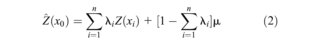
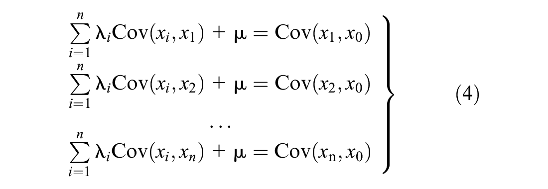
Simple kriging (SK) is the most basic form of kriging in concept and formulation, requiring many assumptions limiting its accuracy and effectiveness ( 14 ). SK assumes sampled values are partial solutions to the random function and that this function is second-order stationary, which implies that any two variate points are dependent on each other based solely on the Euclidean distance between them ( 14 ). The final assumption is unique to SK as it assumes that the mean is known. Ordinary kriging (OK) is the progression from SK, yet is still one of the more simple implementations of kriging and is a functional part of the regression kriging process. The mathematical concept of OK is shown in Equation 1 and the estimator is shown in Equations 2 and 3 below ( 14 , 19 ):

Z (x) = μ + ε (x)

(1)

\hat{Z} (x_{0}) = \sum_{i = 1}^{n} λ_{i} Z (x_{i}) + [1 - \sum_{i = 1}^{n} λ_{i}] μ

(2)

\hat{Z} (x_{0}) = \sum_{i = 1}^{n} λ_{i} Z (x_{i})

(3)

where $\hat{Z} (x_{0})$ is the estimator at the unmeasured location $x_{0}$ , $x_{i}$ are measured locations, and $λ_{i}$ are the weights for the OK estimator that minimizes the variance of the estimator and thus the mean squared error. The weighting values is the positive definite solution of the covariance to the random function. It can be viewed as:

\begin{matrix} \sum_{i = 1}^{n} λ_{i} Cov (x_{i}, x_{1}) + μ = Cov (x_{1}, x_{0}) \\ \sum_{i = 1}^{n} λ_{i} Cov (x_{i}, x_{2}) + μ = Cov (x_{2}, x_{0}) \\ \begin{matrix} \dots \\ \sum_{i = 1}^{n} λ_{i} Cov (x_{i}, x_{n}) + μ = Cov (x_{n}, x_{0}) \end{matrix} \end{matrix}}

(4)

subject to: $\sum_{i = 1}^{n} λ_{i} = 1$

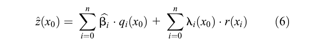
The mean µ is unknown but is assumed to be constant, and the weights applied to the measured data are constrained in that all weights $λ_{i}$ must sum to one. This constraint “filters out” the mean from the estimator because of the restriction on the weights summation ( 14 ) resulting in the simpler Equation 3. This greatly reduces the complexity of the process but still assumes that the mean is constant despite being unknown and filtered out ( 14 ). Naturally, OK shares many of the properties of SK as the only difference between the two is the weight constraint. However, this method does benefit from the estimator not being biased given the weight constraint.

Taking another step beyond OK, the mean remains unknown but is assumed to be non-constant, creating universal kriging (UK). The assumptions in UK are similar to OK, with the addition that the drift of the deterministic values can be modeled using a linear combination of functions, usually polynomial functions of locational attributes ( 14 ). Using polynomials, the weights for UK are determined by minimizing the MSE by employing Lagrange multipliers to determine the weights ( 14 ). The terms UK, RK, and kriging with external drift (KED) all represent the same technique, but with minor differences. This often causes confusion, but RK can be considered the general term that encompasses UK and KED, which have minor differences between them ( 20 ). UK models its drift or trend as a function of the coordinates only, while KED will incorporate or use other auxiliary values ( 20 ). RK makes use of regression modeling to construct a regression function to detrend any external drift and is represented by Equation 5 as follows:

z (x_{0}) = m (x_{0}) + e (x_{0})

(5)

where $m (x_{0})$ is the predicted value from linear regression and $e (x_{0})$ is the residuals that are interpolated using OK ( 19 ). Expanding Equation 5 gives Equation 6 ( 19 )

\hat{z} (x_{0}) = \sum_{i = 0}^{n} \hat{β_{i}} \cdot q_{i} (x_{0}) + \sum_{i = 0}^{n} λ_{i} (x_{0}) \cdot r (x_{i})

(6)

where

\begin{matrix} \hat{β_{i}} = model coefficients \\ q_{i} (x_{0}) & = auxiliary variables \\ \begin{matrix} λ_{i} (x_{0}) \\ r (x_{i}) \end{matrix} & \begin{matrix} = covariance weights \\ = regression residuals \end{matrix} \end{matrix}

From the regression model, the estimates and residuals are calculated and they are then interpolated and added back into the estimated values to obtain the spatially fitted values ( 21 ). This method serves to spatially correct or detrend some model variance (i.e., removing external influences) resulting from the regression model to reduce the MSE value, thus optimizing the model ( 22 ). This method also allows for the inclusion of auxiliary variables for study within kriging’s spatial modeling method thus providing insight into the influence of covariates. It is for this reason this study’s objective is to show how RK can be used in collision modeling while gaining and retaining additional information from auxiliary variables.

Semivariogram Modeling

Before interpolation, the spatial autocorrelation structure of the data needs to be analyzed and understood. The semivariogram helps to define the level of dissimilarity given a lag distance between pairs of data points, and how it changes as the lag increases ( 14 ). Whenever kriging is to be implemented, a semivariogram must be constructed first as a way to quantify the underlying spatial structure of random variables.

The accuracy and quality of the semivariogram is highly contingent on the number of data points. There have been many suggested minima, some as low as 25, but Oliver and Webster ( 21 ) suggest the minimum of 100 data points is optimal but can be lower if data density is dispersed. Another factor affecting the accuracy would be directionality, where the data will show some form of anisotropic tendency meaning there is a stronger spatial association in a particular direction ( 14 , 22 ) and may require additional investigation. However, when not accounting for directionality it is called omnidirectional and assumes that there is no spatial directionally to the variance structure in the semivariogram.

Additionally, a stationarity assumption is made which assumes that the distribution or data variation is consistent throughout the study area and does not change from location to location or from small to large spatial scales ( 14 , 22 ). Known as a second-order stationarity assumption, it states that the covariance depends on the separation distance only and that the mean is constant even if this is not completely true in the real world ( 22 ).

Logically, as the distance between two data points increases, so does the level of dissimilarity between them, and this should be reflected in the empirical semivariogram plot. This is a plot of the correlation between two points over the distance between them and can be done either by point to point or more commonly via lags.

A functional semivariogram is fitted to the plot and is the mathematical representation of the autocorrelation structure. Of the many functions that have been developed, the three common semivariogram functions are spherical, exponential, and Gaussian, as shown in Equations 7 to 9, respectively.

Sph (h) = {\begin{matrix} C (\frac{3 h}{2 a} - \frac{1}{2} \cdot {(\frac{h}{a})}^{3}) & 0 \leq | h | \leq | a | \\ C & | a | \leq | h | \end{matrix}}

(7)

Exp (h) = C (1 - e^{- \frac{3 h}{a}})

(8)

Gau (h) = C (1 - e^{- 3 {(\frac{h}{a})}^{2}})

(9)

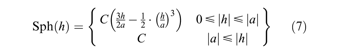
Other less commonly used semivariogram functions include cubic, sine hole, and pentaspherical ( 23 ).

Once a semivariogram function is chosen, it is then used in the process of calculating the distance-based weights. Each mathematical model used in this study provides three important values: the nugget, the range, and the sill. The nugget is the measurement error or variation that is associated with the data collection and manifests as the gap from the origin to the y-intercept, even though it should ideally be zero. Since data collections and measurements are seldom perfect, the nugget will usually have an effect on the value of the sill, shifting it upwards. The range is the distance value where the level of dissimilarity flattens out or reaches a plateau, and the sill is the value of this plateau. Figure 1 represents a typical semivariogram plot:

Figure 1.

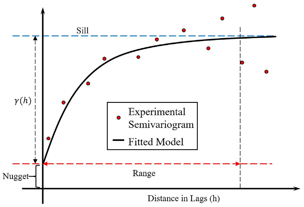
Typical semivariogram plot with a fitted model.

Another variable, known as the partial sill or p-sill, is the difference between the sill and the nugget value. This is a simple subtraction to better illustrate the theoretical sill when the nugget should ideally be zero.

The semivariogram should represent the change in correlation based solely on distances, but in some cases external factors may influence the level of drift or trend in the data ( 14 ). It is important that these external factors are accounted for to isolate the spatial aspect. It is only when the spatial factor is isolated that the optimal semivariogram function can be chosen and then the kriging interpolation can done to generate a series of estimated or predicted values.

Cross-validation is often used as a measure of how accurate and reliable the generated model is. This is done by removing one data point and then using the model and the surrounding variables to calculate an estimate at that point, and the associated variances ( 22 ). This is repeated for all data points in the dataset and the results are then used to calculate comparison statistics using three error metrics: mean squared error (MSE), root mean squared error (RMSE), and root mean squared standardized error (RMSSE), to interpret the goodness of the model ( 22 ). MSE represents the average of the squares of error and is often used to measure the quality of an estimator, whereas RMSE is used to measure the accuracy of a model. RMSSE is used to examine the variability of the estimations (under- or over-estimations). Generally, the suitable model would yield MSE and RMSE values close to zero and RMSSE values close to one. All three error types are expressed by the following Equations 10 to 12.

MSE = \frac{1}{n} \sum_{i = 1}^{n} [\frac{Z^{*} (x_{i}) - Z (x_{i})}{σ^{2} (x_{i})}]

(10)

SE = \sqrt{\frac{1}{n} \sum_{i = 1}^{n} {[Z^{*} (x_{i}) - Z (x_{i})]}^{2}}

(11)

RMSSE = \sqrt{\frac{1}{n} \sum_{i = 1}^{n} {[\frac{Z^{*} (x_{i}) - Z (x_{i})}{σ^{2} (x_{i})}]}^{2}}

(12)

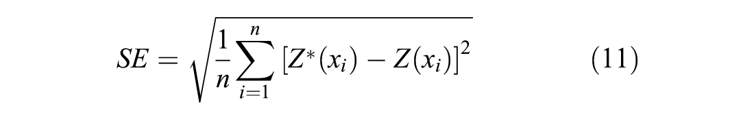
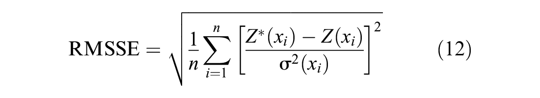
where $σ^{2} (x_{i})$ , $Z^{*} (x_{i}), Z (x_{i})$ denote the kriging variance, the estimated and the measured values of the random variable at location $x_{i}$ , respectively.

Methodology

This section outlines the methodology undertaken in this study. Given the amount and variety of data being used and the calculations being done, select software and scripting packages were used. To improve the mapping accuracy and reduce the complexity associated with handling spatial data used in this study, all the datasets are processed and spatially aggregated using one of the most established and well-known geographic information system (GIS) platforms, Esri’s ArcGIS ( 19 ). Data management, tables, and descriptive statistics were handled using Microsoft Excel. Calculations were handled using a combination of R and Python.

Data Collection and Processing

Collision Data

Given the randomness and independent nature of collisions, it is important to have a sufficient sample size and quality of collision data. As required for spatial analysis, the collision data should also be geocoded or at least have some form of coordinates associated with them. Additionally, weather and road conditions should also be a part of the collision data set for each collision as those categorical variables will be the basis for categorizing the collisions as winter condition based or not. Most transportation authorities maintain a regularly updated collision record database online that is freely available and easily obtainable. The collision data need to be processed to isolate the collisions that take place in the time frame and study area. Additionally, this would also be a good time to do a preliminary analysis of the collision record with descriptive statistics as it may reveal additional clues as to the auxiliary variables that may be used.

Meteorological and Road Conditions Data

Meteorological and road surface condition data is often collected remotely and automatically via a system of automatic weather stations or sensors. For this study, the Iowa Environmental Mesonet database, maintained by Iowa State University, is the source of all environmental data used from the various data collection networks. One type of automated system used is the Road Weather Information System (RWIS) which is a collection of advanced meteorological instruments, road surface sensors, and a communication system in which it reports the local weather and road condition ( 24 ). Another weather information collection system used is the National Weather Service Cooperative Observer Program (NWS-COOP), which is a network of individuals that collect and record daily weather observations and is often used as a baseline to compare against remote sensing methods. The information on weather and road surface conditions requires more work and should be scrutinized for consistency and completeness. It is not uncommon for a weather station or road sensor to stop reporting for a period of time because of malfunctions in the system. This may result in the data being reported to be either far out of the range of normality or not even reported at all. The amount of missing and erroneous data (e.g., extreme temperatures) should be kept to a minimum and any station or sensor whose data does not meet the minimum requirements for completeness should be omitted from the analysis.

Road Network

The final piece of data required for this study would be the road network, for which the collisions that took place also need to be spatially matched to the same spatial coordinate system as the collision data. This not only provides a visual representation of the collisions but also provides additional characteristics that may be used for the collision analysis. However, this study focuses exclusively on the effects of winter conditions on collisions, thus the physical properties of the road network are omitted. It is important to use as complete a road network as possible and to ensure that the quality of the file is as high as possible to reduce the need for data cleanup and error correction. All the various data used in the analysis should be set to the same space and coordinate system to make spatial joining simpler and to reduce any possible errors. The road network being used should be segmented into uniform lengths to provide a consistent collision space throughout the network. The segments should be long enough to reduce the network complexity, while short enough to retain a level of spatial granularity.

Spatial Data Aggregation

Collision data are often sparse and spread-out, thus multi-year averages are often used to analyze collision statistics to observe groupings or clusters for hot spot analysis. The time period for this study is five winter seasons and the overall total number of collisions and the total number of winter collisions are aggregated to the road segment on which they occur.

To calculate winter collisions (WC) as a proportion of all collisions, the ratio of WC over all collisions for each road segment is calculated and will be the dependent variable for the analysis. This follows the method implemented by Khan et al. ( 25 ) who utilized a ratio of various adverse driving condition collisions to all collisions as a measure of relative collision frequency for the road condition, providing a relationship between WC and non-WC collisions from a purely condition standpoint. A high WC ratio is an indicator of a road segment that is riskier during adverse weather/surface conditions than segments with a lower WC ratio when exposed to the same weather/surface conditions. Following Khan et al. ( 25 ) and Heqimi et al. ( 26 ), a collision is deemed a WC if the reported contributing surface condition includes snow, ice, frost, or slush; or if the reported weather condition at time of collision was snow, freezing rain, blowing snow, or sleet/hail.

There will be some road segments where there are no collisions reported and these will throw an error when doing the ratio calculation as dividing by zero is undefined. Additionally, reporting the road segment as a zero-ratio is also incorrect, as the meaning behind a zero-ratio is very different than having zero collisions. These road segments with “null” WC ratios are effectively segments with “no data” and thus are treated as such.

The meteorological data is also aggregated to be a five-year seasonal average and projected onto the road segments. Given the point data nature of the weather stations used, the meteorological variables will need to be spatially interpolated to obtain a continuous surface map of the meteorological variables that can then be aggregated onto the road segments of the road network. It was shown by Kwon and Gu ( 24 ) that the road surface temperature may be interpolated between RWIS stations using kriging within reason, and Eguía et al. ( 27 ) showed that spatial interpolations of meteorological data can also be done with the application of kriging. Weather events such as precipitation can also be interpolated using OK and indicator kriging, as was done by Atkinson and Lloyd ( 28 ) in mapping precipitation in Switzerland. Therefore OK was applied to all station variables statewide to obtain a data surface map, which was then converted to a raster file to extrapolate the estimated values. The raster values were then averaged onto a 1 km × 1 km grid over the road network to reduce the overall data points while maintaining a higher level of granularity and to facilitate projection onto the road line segments.

Spatial Interpolation via RK

Since kriging works best as point data analysis, the road segments were collapsed to their mid-points and their coordinates were added to the attributes table. Once the data is reduced to point form, then RK can be implemented on the dataset. Applying RK involves all the traditional steps involved with multiple linear regression such as correlation analysis and the stepwise variable selection process. Once the regression model is found, the predicted results and their residuals are calculated. The next step in this process is to perform a semivariogram analysis and an OK interpolation on the residuals. The interpolated residuals are then added back onto the predicted regression results to obtain the final RK values. Figure 2 is a flowchart representing the RK process and was adapted from the study by Peng et al. ( 29 ) with spatial distribution of organic soils. Once the RK values have been calculated, then the MSE, RMSE, and RMSSE can be found via cross-validation to determine the performance of the developed models as discussed above.

Figure 2.

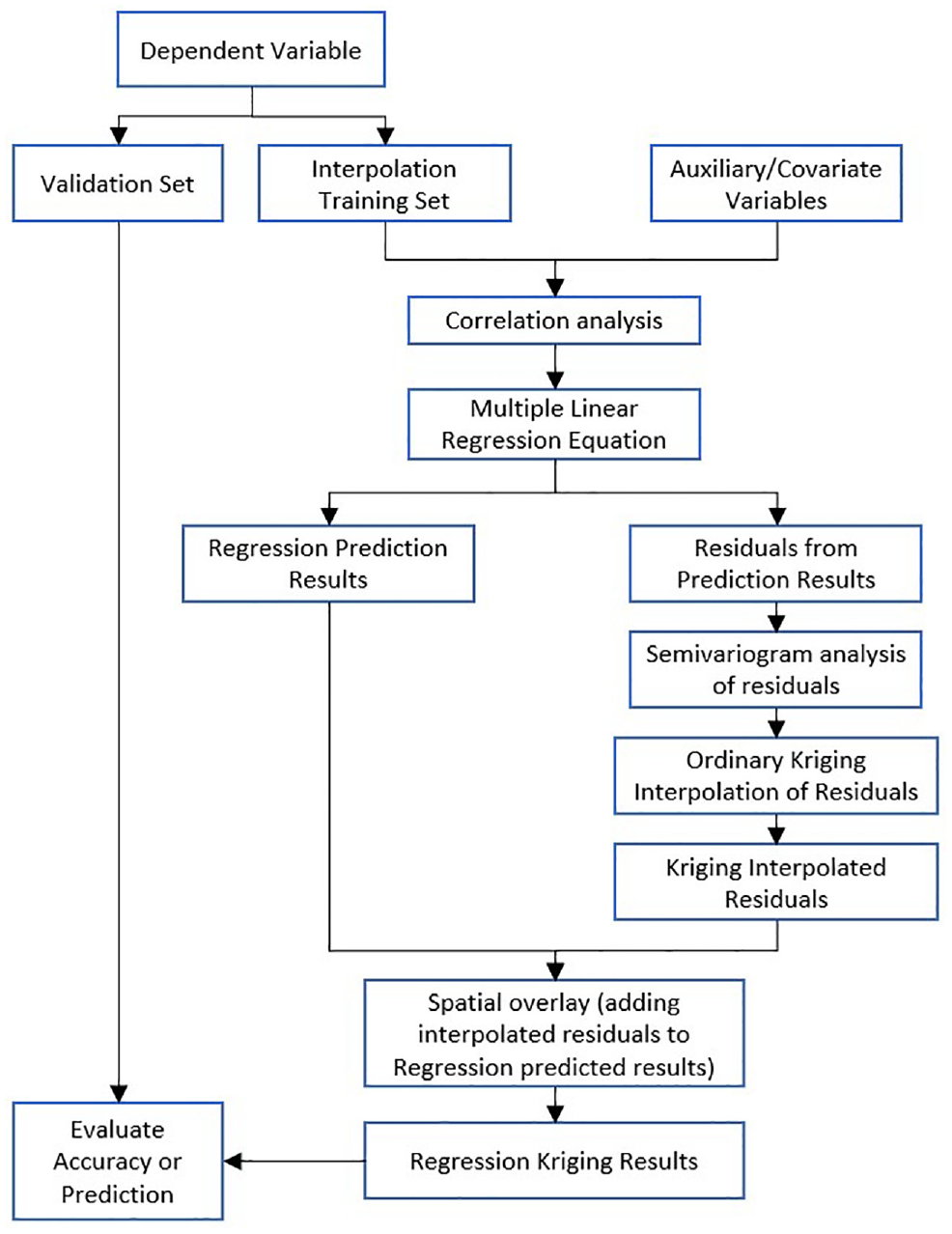
Regression kriging process flowchart.

Case Study

Study Area

The proposed method is applied to a case study exploring the effectiveness of RK in finding the potential spatial relations of WC proportions within the northeast quadrant of the State of Iowa. This study focuses on the aggregated collisions over five winter seasons from the winters of 2013/14 to 2017/18 and is limited to major roads (MRD) such as Interstates, state, and local highways. Figure 3 depicts the study area in the northeast quadrant of Iowa spanning over 45,279 km² and the 4,255 km of roads used. The study period encompasses the winter months of December to February as defined by the U.S. National Oceanic and Atmospheric Administration (NOAA) ( 30 ) and the shoulder months of October, November, and March, as they represent a period of transition between the summer and winter seasons. Other months were omitted as they did not have sufficient amounts of winter weather conditions reported.

Figure 3.

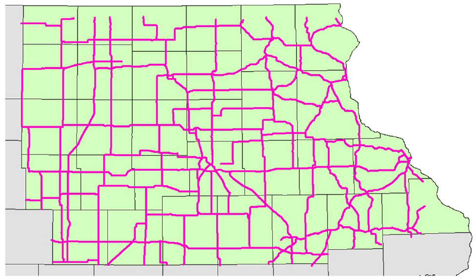
Iowa counties: case study area and road network.

Data Processing and Integration

The collision data and the road network shapefile were obtained from the Iowa Department of Transportation (DOT) open data portal ( 31 ). The collision dataset is a record of all reported collisions within the state for a period of 10 years and the road network file contains the majority of roads in Iowa from Interstates to forestry service roads and contains road geometry and AADT information. The weather and road surface condition information was also obtained for the study period to see if the WC ratio can be better estimated with the help of these covariates or auxiliary variables. The database used was the Iowa Environmental Mesonet maintained by Iowa State University ( 32 ). Daily climate data came via NWS-COOP records and Iowa’s network of RWIS provided additional climate data as well as road surface condition information and warning statuses as archived by the Mesonet database. For each dataset, the completeness and availability of the data was checked and any station that had less than 70% of data for either condition was omitted from the analysis, as there were instances where some stations had no readings for months because of maintenance or technical problems.

To reduce complexity and the size of the dataset, the road network was pared down to major roads only, such as Interstates and state and local highways. Given the state of the road network file, the network lines were dissolved into a uniform, single line road network. This single feature was then segmented into 5.0 km, or smaller, lengths. This resulted in 1,225 segments of road with an average length of 3.7 km.

The collisions included in the analysis are those that occurred in the study area within the study period and that occurred on the major roads selected. The number of collisions on each segment of road was summed and added to the segment’s attributes table. Following the previously defined conditions for a WC classification, these collisions were tabulated and assigned to the road segments and then the WC ratio was calculated. The WC ratio will be the dependent variable in the regression analysis and the variable of interest for the RK interpolation.

The road condition warning messages were color coded based on their level of severity for winter roads. Road surface condition color codes currently used by the Minnesota DOT ( 33 ) and many other state DOTs are shown in Figure 4. For the intended analyses, collisions that occurred when either of the three top warning levels (e.g., red, orange, and yellow) were in effect are treated as road weather related collisions (i.e., winter collisions) and thus used in the study.

Figure 4.

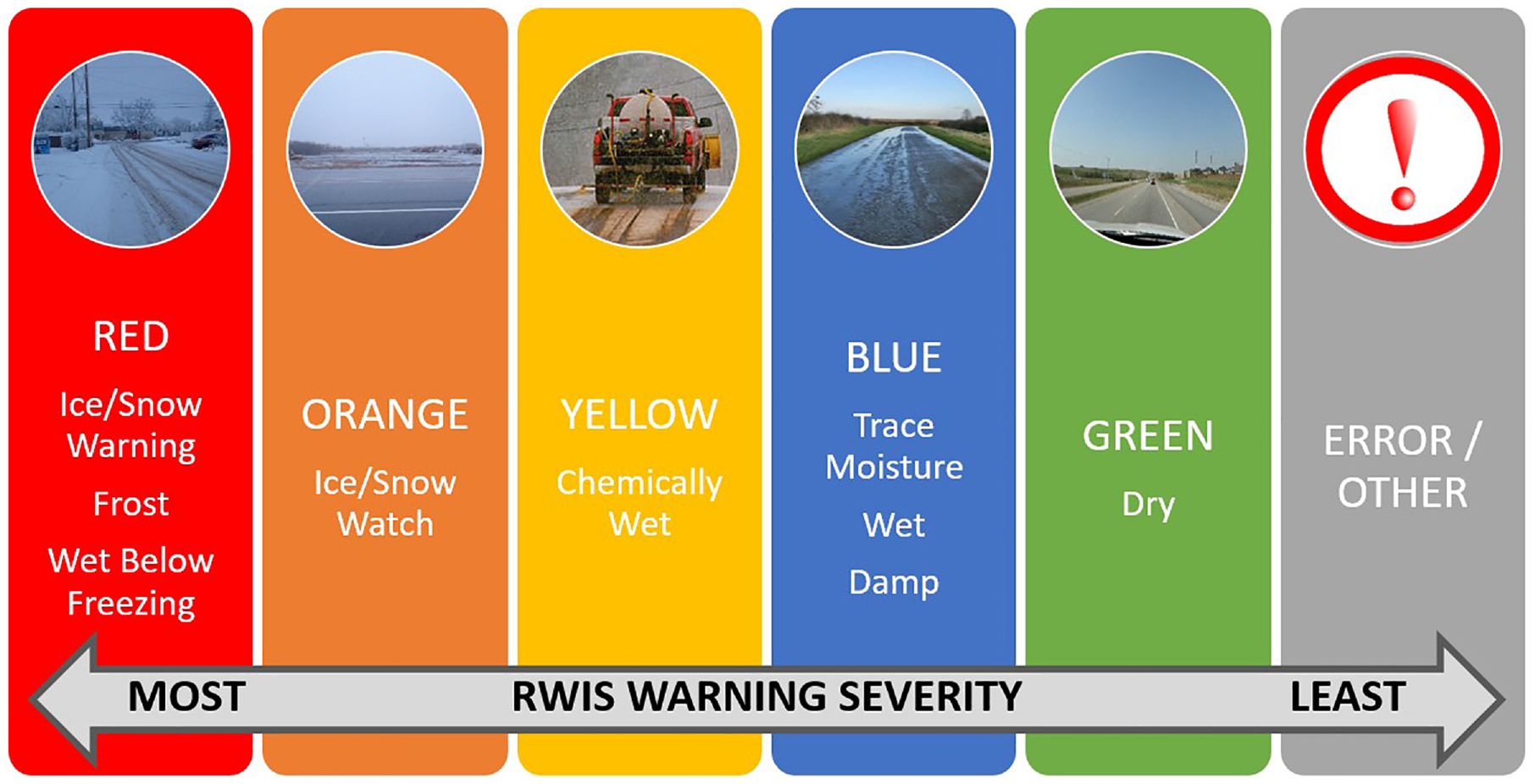
Road weather information systems (RWIS) road surface warning color codes.

The selected meteorological data was processed and interpolated using OK by following the steps discussed in the previous section. The RWIS variables used were: road surface temperature (RST), air temperature, and road condition warning messages. Variables used from the NWS-COOP were the daily snowfall totals, daily high air temperature, and daily low air temperature.

Table 1 provides the descriptive statistics for the variables used over the five winter seasons, equating to 30 months of aggregated data collection. Figure 5 shows the interpolated surface maps for the meteorological variables.

Table 1.

Descriptive Statistics of Meteorological Variables Considered in the Study

	Average monthly road surface temperature	Average monthly air temperature	Average monthly red warnings	Average monthly orange warnings	Average monthly yellow warnings	Snowfall totals	Average daily high temperature	Average daily low temperature
Unit	°C	°C	Count	Count	Count	cm	°C	°C
Number of stations	33	33	33	33	33	128	128	128
Min.	−7.9	−8.5	0	0	0	0	−10.2	−21.6
Mean	2.7	1.0	100	875	30	5.1	5.4	−5.5
Max.	14.9	14.8	990	2481	213	34.7	21.5	10.7
SD	6.1	6.2	133	632	33	5.6	7.5	6.8

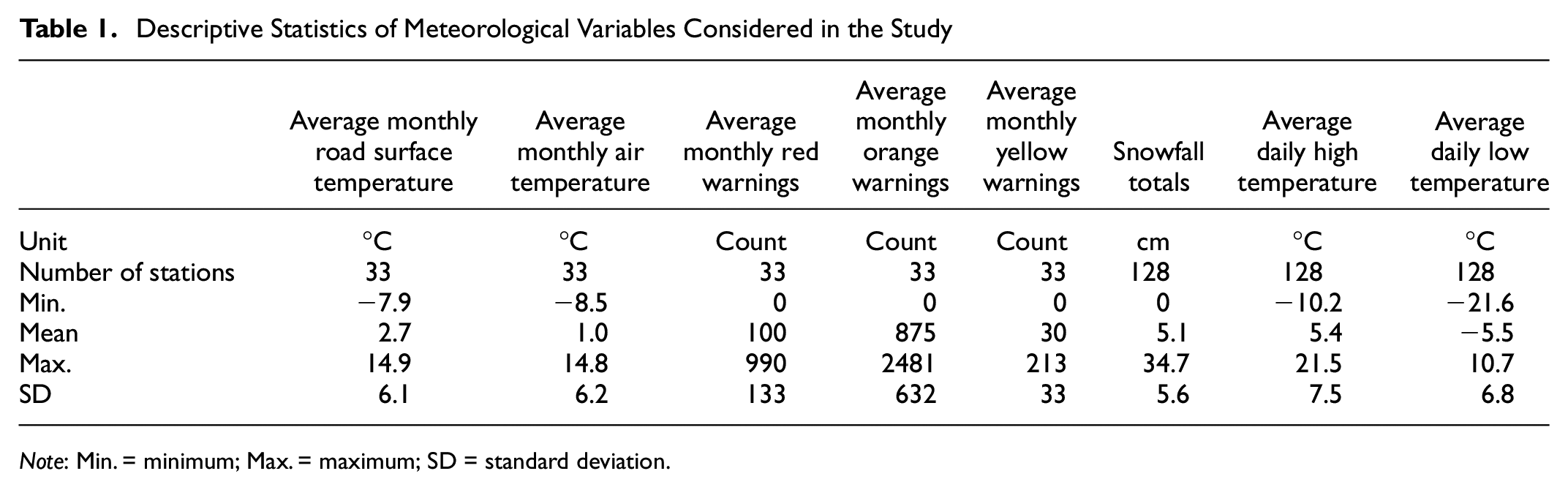
Note: Min. = minimum; Max. = maximum; SD = standard deviation.

Figure 5.

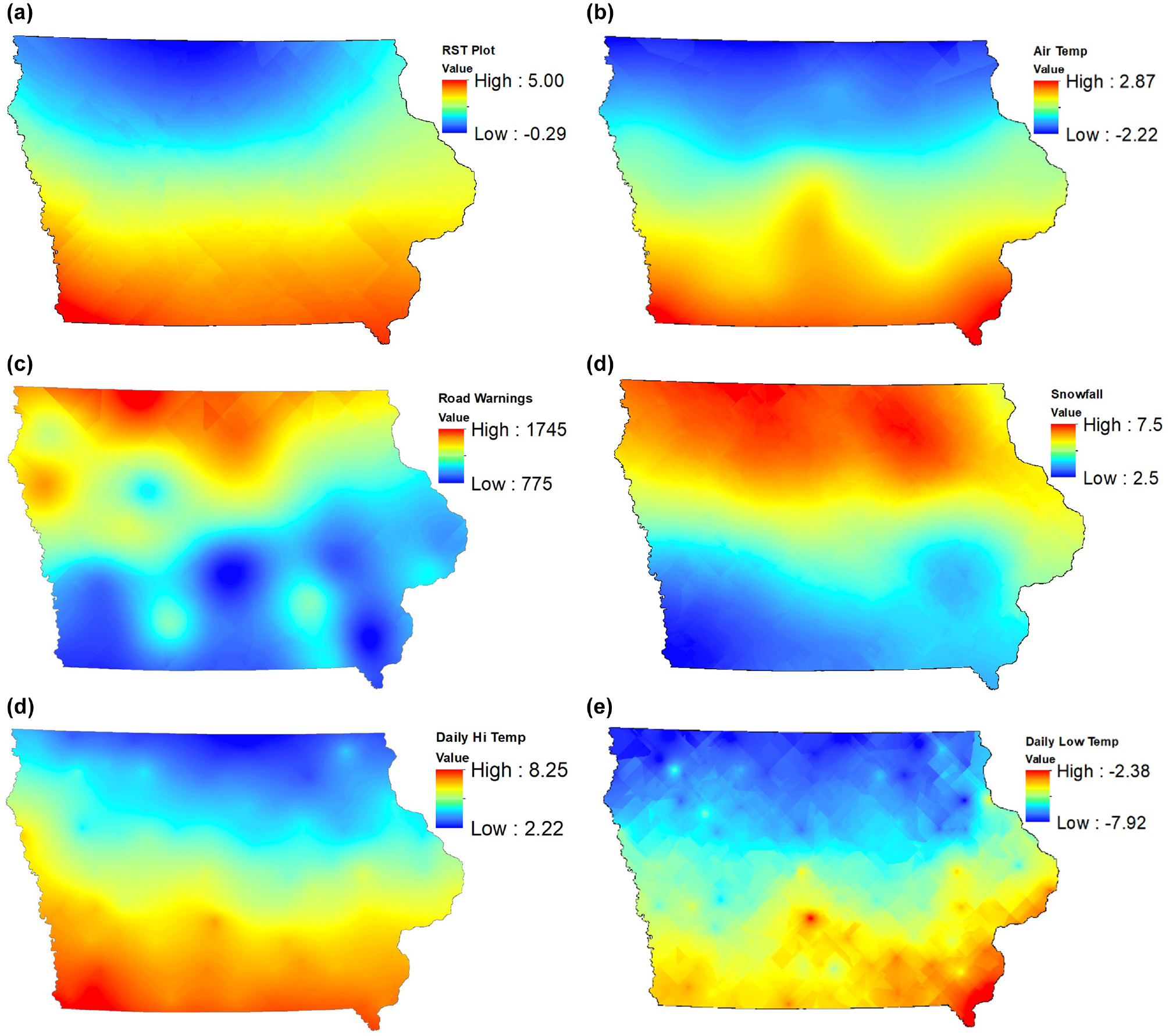
Kriged surface maps for variables considered in this study: (a) seasonal average road surface temperature (RST) (°C), (b) average monthly air temperature (°C), (c) sum of red, orange, and yellow road warning messages, (d) average seasonal snowfall totals (cm), (e) average daily high temperature (°C), and (f) average daily low temperature (°C).

All the interpolated surface maps were converted into a raster file so that the values may be projected onto the road. Each road segment averages out all the interpolated points for that road segment. Once the collision and meteorological data have been attached to the road segments, the RK process may begin.

Hot spot Analysis via RK

Following the method outlined previously, the regression analysis was first done on the geoprocessed data. To ensure model accuracy and validity, a correlation matrix analysis was done to ensure that no two-pair collinearity is present within the independent covariates. A variance inflation factor (VIF) analysis was done to assess if any multicollinearity is present. Covariates with VIF values greater than 10 indicate severe multicollinearity and should be removed from the model ( 34 ). A logarithmic transformation was done on the annual average daily traffic (AADT) count to address their large values and potential non-linear relationship. Once independence from each other was verified, a stepwise regression analysis was done to obtain the final multiple linear regression model at a 95% confidence interval. The final variables are presented in Table 2.

Table 2.

Multiple Linear Regression Results

	Coefficient estimate	Standard error	\|t-Value\|	P-value against α = 0.05	Variance inflation factor (VIF)
Linear regression
Intercept	0.2723	0.1469	1.854	0.06403	na
log Annual Average Daily Traffic (ln AADT)	0.0372	8.96E−03	4.145	3.65E−05	1.137
Road Surface Temperature (RST)	−0.2204	0.0290	−7.593	6.55E−14	7.916
Air temperature	0.1353	0.0255	5.319	1.26E−07	6.150
Red warnings	−4.35E−04	1.50E−04	−2.9	0.00381	2.829
Orange warnings	1.85E−04	9.14E−05	2.026	0.04305	2.367

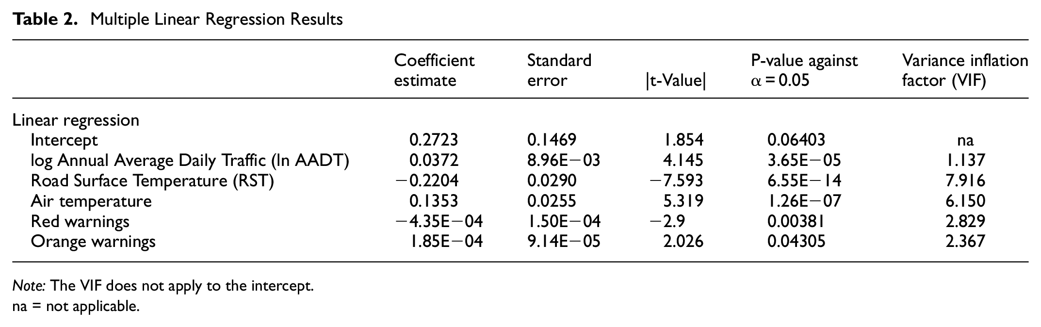
Note: The VIF does not apply to the intercept.na = not applicable.

The results show that lnAADT, RST, Air Temperature, and red and orange color-coded warnings are variables that have some statistical correlation with the WC ratio. These results are intuitive, as AADT is directly proportional to the WC ratio and the RST and number of red warnings are inversely proportional to the WC ratio. The inverse relationship between red warnings and collision ratios seems counter-intuitive, but it should be noted that RWIS stations are used by WRM to identify hazardous conditions and are often connected to digital road warning signs, and red conditions are usually visually obvious. It can be surmised that an increase in warnings will lead to more WRM activities, and the alert messages lead to drivers adjusting to the road conditions ahead. Air temperature does not seem intuitive at first until one recalls that the time frame is over the winter months and that the formation of ice on the road surface requires some melting of ice or snow on the roadside that will then re-freeze, usually overnight. Though more investigation is required, the trend that an increase in air temperature over the winter may result in a higher WC ratio is most likely a result of ice formation.

Following the next step in the RK process, the semivariogram of the residuals were generated using gstat package of R. Figure 6 shows the empirical semivariogram plots and fitted models generated:

Figure 6.

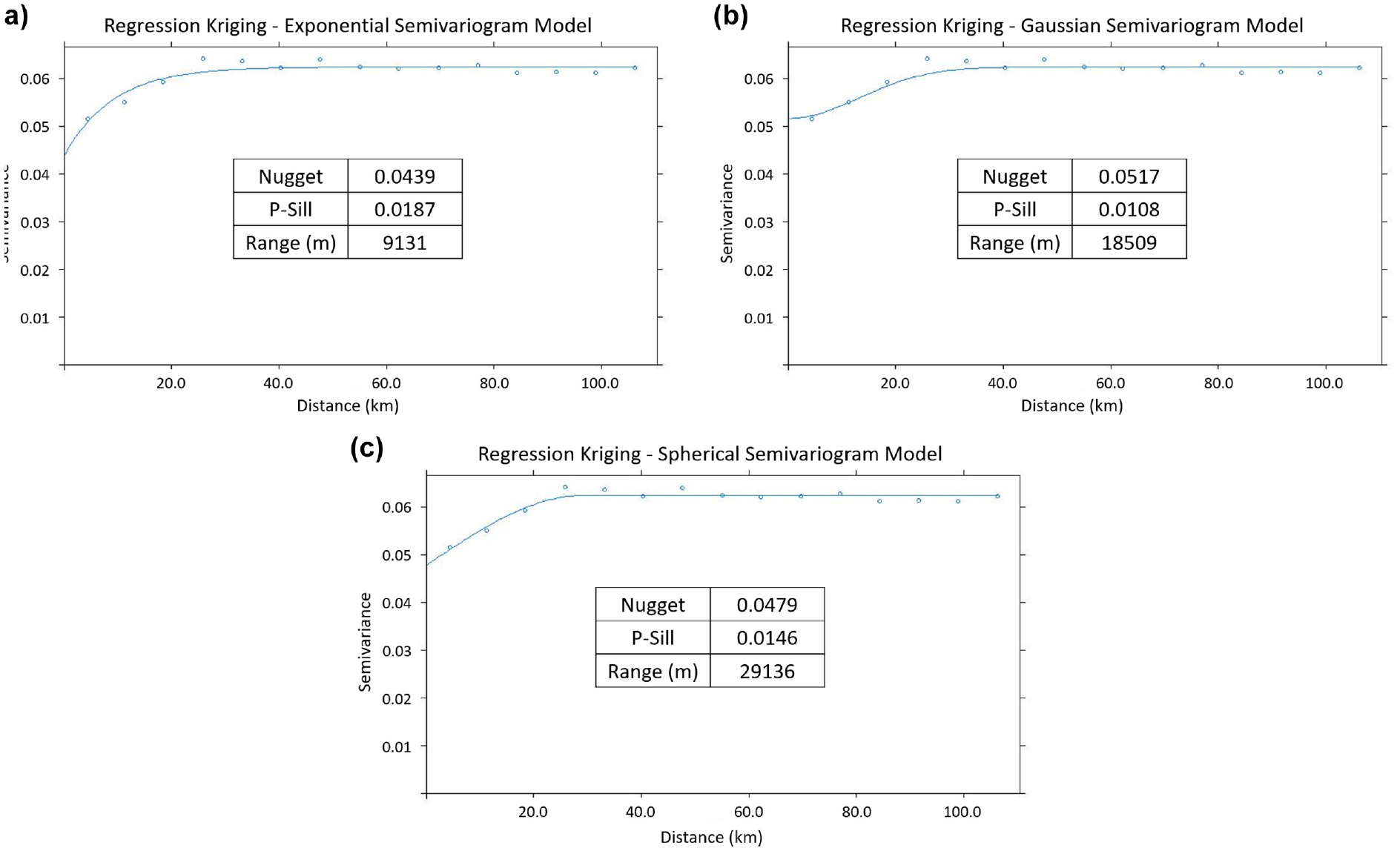
Semivariogram plots of the winter collision (WC) ratios’ residuals: (a) exponential model semivariogram, (b) Gaussian model semivariogram, and (c) spherical model semivariogram.

Visually obtaining the nugget, sill, and range from the plots can be difficult at times, but the gstat package in R provides that information as part of the algorithm ( 35 , 36 ). Cross-validation was completed for each model and the average results of the MSE, RMSE, and RMSSE values were 0.061, 0.247, and 0.847 respectively. These three performance metrics indicate that all the models satisfy the model conditions for a good predictor. Of the three models presented, it is in the nugget analysis where the exponential model appears to be a better fit. With smaller nugget value, the inherent measurement error is reduced in exchange for a smaller predictive spatial range. This model was used to generate a hot spot plot.

Figure 7 is the final hot spot map for the WC ratios modeled using five quantile risk levels for visualization purposes. These values can easily be validated by looking at the measured ratios as found on those sections and how they compare with the overall average. This plot shows low- to high-risk segments of roads that could potentially be used by the respective WRM authorities for further diagnoses and provide recommendations including possible preventative treatments, increased WRM activities, socioeconomic appraisals, or for study into transportation policy changes. By doing so, in return it will reduce the winter weather related collisions and improve the safety of the traveling public during inclement weather events.

Figure 7.

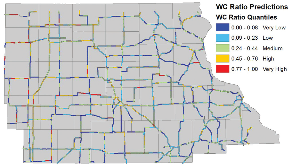
Winter collision (WC) ratio hot spot plot.

Conclusion and Future Work

Winter driving conditions pose a real problem in some countries, where transport agencies work to keep the roads safe for the general public. Slippery roads and adverse weather conditions make driving riskier for drivers and road authorities try to reduce the risk with either regular maintenance activities or with engineered strategies. Given how expensive and time consuming these activities are, targeted implementation is key to maximizing their impact and efficiency. Thus, targeting road segments that display a high ratio of winter condition collisions to all collisions during the winter months can help reduce the number of collisions overall by reducing the number of WC. The findings are summarized below:

Before applying RK, the covariates being studied needed first to be spatially interpolated using OK. Once completed, it was used within RK as auxiliary variables for modeling the WC ratios throughout the road network. From this process, it was found that RK performs well based on the nugget, MSE, RMSE, and RMSSE values from the cross-validation conducted in the analysis process.

RK allowed us to determine auxiliary variables that help to improve model performance and accuracy, namely AADT, RST, and number of red level warnings. The variables are intuitive, as higher AADT usually means higher exposure rates and RST can indicate the potential for slippery conditions thus correlating with an increased number of collisions. Understanding what auxiliary variables contribute to WC also provides insight into the possible relationships between these variables and WCs. Though this type of analysis is considered reactionary (modeling what has already happened), it may be used to predict possible problematic locations.

This method can be useful for road authorities that have limited collision records or where record keeping is not robust and detailed. Kriging makes use of spatial correlation that is often not accounted for in the more traditional analysis methods and as shown here, the spatial correlation alone can be used effectively to model WC ratio hot spots over a large area with a large road network. Hot spot mapping will visually aid municipalities and road authorities in making more informed decisions with regard to their WRM programs.

Some suggestions for further research are:

A comparative benchmarking of RK against more established methodologies will follow this paper to determine its relative effectiveness.

Expansion and inclusion of additional weather sources can be used to further improve the accuracy of spatial interpolations of weather variables, such as the automated surface/weather observing systems (ASOS/AWOS) network for air traffic and the proprietary maintenance decision support system (MDSS) network.

Auxiliary variables were limited to meteorological conditions over the road network, however, it is well known that road geometry and road speeds play an important role in collisions. Therefore including road characteristics may improve the regression models and thus the RK.

The inclusion of interaction terms between covariates could be included in future RK analysis.

Given the limitations mentioned with linear regression, implementing negative binomial regression may provide improvements in the RK outcome.

This study assumes stationarity holds; therefore, research into this assumption could help determine if the spatial scale can be further increased to the whole state.

Further research into the effectiveness of RWIS may also provide insight into correlation between road warnings and their effects on collision frequencies.

Footnotes

Acknowledgements

The authors would like to thank the Iowa Department of Transportation and Iowa Environmental Mesonet of Iowa State University for providing the necessary data to complete this study.

Author Contributions

The authors confirm contribution to the paper as follows: study conception and design: A. Wong, T. J. Kwon; data collection: A. Wong; analysis and interpretation of results: A. Wong, T. J. Kwon; draft manuscript preparation: A. Wong, T. J. Kwon. All authors reviewed the results and approved the final version of the manuscript.

Declaration of Conflicting Interests

The author(s) declared no potential conflicts of interest with respect to the research, authorship, and/or publication of this article.

Funding

The author(s) received no financial support for the research, authorship, and/or publication of this article.

ORCID iDs

Andy H. Wong

Tae J. Kwon

References

How Do Weather Events Impact Roads?, Federal Highway Administration. 2020. https://ops.fhwa.dot.gov/weather/q1_roadimpact.htm. Accessed July 25, 2020.

Asano

Hirasawa

Characteristics of Traffic Accidents in Cold, Snowy Hokkaido, Japan. Proceedings of the Eastern Asia Society for Transportation Studies, Vol. 4, 2003, pp. 1426–1434.

Pennelly

Reuter

G. W.

Tjandra

Effects of Weather on Traffic Collisions in Edmonton, Canada. Atmosphere-Ocean, Vol. 56, No. 5, 2018, pp. 362–371.

Thakali

Kwon

T. J.

Usman

A Risk-Based Approach to Winter Road Surface Condition Classification. Canadian Journal of Civil Engineering, Vol. 44, No. 3, 2017, pp. 182–191.

Eisenberg

Warner

K. E.

Effects of Snowfalls on Motor Vehicle Collisions, Injuries, and Fatalities. American Journal of Public Health, Vol. 95, No. 1, 2005, pp. 120–124.

Andrey

J. C.

Mills

B. E.

Collisions, Casualties, and Costs: Weathering the Elements on Canadian Roads, 1st ed. Institute for Catastrophic Loss Reduction, London, ON, Canada, 2003.

American Association of State Highway and Trasnsportation Officials. Highway Safety Manual Vol. 1, 1st ed. Washington, D.C.: AASHTO, 2010.

Islam

M. T.

El-Basyouny

Ibrahim

S. E.

Sayed

Before–After Safety Evaluation Using Full Bayesian Macroscopic Multivariate and Spatial Models. Transportation Research Record: Journal of the Transportation Research Board, 2016. 2601: 128–137.

Thakali

Kwon

T. J.

Identification of Crash Hotspots Using Kernel Density Estimation and Kriging Methods: A Comparison. Journal of Modern Transportation, Vol. 23, No. 2, 2015, pp. 93–106.

10.

Nicholson

Analysis of Spatial Distributions of Accidents. Safety Science, Vol. 31, 1999, pp. 71–91.

11.

Levine

Kim

K. E.

Nitz

L. H.

Spatial Analysis of Honolulu Motor Vehicle Crashes: I. Spatial Patterns. Accident Analysis and Prevention, Vol. 27, No. 5, 1995, pp. 663–674.

12.

Black

W. R.

Thomas

Accidents on Belgium’s Motorways: A Network Autocorrelation Analysis. Journal of Transport Geography, Vol. 6, No. 1, 1998, pp. 23–31.

13.

Harirforoush, H., and L. Bellalite. A New Integrated GIS-based Analysis to Detect Hotspots: A Case Study of the City of Sherbrooke. Accident Analysis and Prevention, Vol. 130, 2019, pp. 62–74.

14.

Olea

R. A.

Geostatistics for Engineers and Earth Scientists. Springer Science + Business Media, New York, 1999.

15.

Selby

Kockelman

Spatial Prediction of AADT in Unmeasured Locations by Universal Kriging. Transportation Research Board, Washington, D.C., 2011.

16.

Einax

J. W.

Soldt

Geostatistical and Multivariate Statistical Methods for the Assessment of Polluted Soils—Merits and Limitations. Chemometrics and Intelligent Laboratory Systems, Vol. 46, 1999, pp. 79–91.

17.

Cressie

The Origins of Kriging. Mathematical Geology, Vol. 22, No. 3, 1990, pp. 239–252.

18.

Manepalli

U. R.

Bham

G. H.

Crash Prediction: Evaluation of Empirical Bayes and Kriging Methods. Proc., 3rd International Conference on Road Safety and Simulation, Indianapolis, IN, 2011, pp. 1–13.

19.

ESRI. ArcGIS Desktop: Release 10. Environmental Systems Research Institute, Redlands, CA, 2011.

20.

Hengl

Heuvelink

G. B.

Stein

A Generic Framework for Spatial Prediction of Soil Variables Based on Regression-Kriging. Geoderma, Vol. 120, No. 1–2, 2004, pp. 75–93.

21.

Zhu

Lin

H. S.

Comparing Ordinary Kriging and Regression Kriging for Soil Properties in Contrasting Landscapes. Pedosphere, Vol. 20, No. 5, 2010, pp. 594–606.

22.

Oliver

M. A.

Webster

Basic Steps in Geostatistics: The Variogram and Kriging. Springer International Publishing, New York, NY, 2015.

23.

Olea

R. A.

A Six-Step Practical Approach to Semivariogram Modeling. Stochastic Environmental Research and Risk Assessment, Vol. 20, No. 5, 2006, pp. 307–318.

24.

Kwon

T. J.

Modelling of Winter Road Surface Temperature (RST)—A GIS-Based Approach. Proc., 2017 4th International Conference on Transportation Information and Safety (ICTIS), Banff, Alberta, Canada 2017, pp. 551–556.

25.

Khan

Qin

Noyce

D. A.

Spatial Analysis of Weather Crash Patterns in Wisconsin. Journal of Transportation Engineering, Vol. 134, No. 5, 2008, pp. 191–202.

26.

Heqimi

Kay

J. J.

Gates

T. J.

Using Spatial Interpolation to Determine Effects of Snowfall on Traffic Crashes: A Case Study of Interstate-94 in Southwest Michigan. Presented at TRB 96th Annual Meeting Compendium of Papers DVD record, Washington, D.C., Michigan, United States, 2017.

27.

Eguía

Granada

Alonso

J. M.

Arce

Saavedra

Weather Datasets Generated Using Kriging Techniques to Calibrate Building Thermal Simulations with TRNSYS. Journal of Building Engineering, Vol. 7, 2016, pp. 78–91.

28.

Atkinson

P. M.

Lloyd

C. D.

Mapping Precipitation in Switzerland with Ordinary and Indicator Kriging. Journal of Geographic Information and Decision Analysis, Vol. 2, No. 2, 1998, pp. 72–86.

29.

Peng

Bing

Guangpo

Guangcan

Spatial Distribution of Soil Organic Carbon and Total Nitrogen Based on GIS and Geostatistics in a Small Watershed in a Hilly Area of Northern China. PLoS One, Vol. 8, No. 12, 2013, p. e83592.

30.

NOAA. Iowa Climate Normals Map. National Oceanic and Atmospheric Administration. May 16, 2020. https://www.weather.gov/dmx/climatenormals.

31.

Iowa Department of Transportation. Iowa DOT Open Data. May 31, 2020. https://public-iowadot.opendata.arcgis.com/

32.

Iowa State University. Iowa Environmental Mesonet. January 6, 2020. https://mesonet.agron.iastate.edu/.

33.

Minnesota Department of Transportation. SCAN Glossary. MnDOT SCAN Web 6.0. July 25, 2020. http://rwis.dot.state.mn.us/scanweb/SWFrame.asp?Pageid=Home&Units=&Groupid=&DisplayClass=Java&SenType=All. Accessed July 25, 2020.

34.

Montgomery

D. C.

Peck

E.A.

Vining

G. G.

Introduction to Linear Regression Analysis, 3rd ed. John Wiley & Sons, Inc., New York, 2001.

35.

Pebesma

E. J.

Multivariable Geostatistics in S: The gstat Package. Computers & Geosciences, Vol. 30, 2004, pp. 683–691.

36.

Gräler

Pebesma

Heuvelink

Spatio-Temporal Interpolation Using gstat. The R Journal, Vol. 8, No. 1, 2016, pp. 204–218.

Development and Evaluation of Geostatistical Methods for Estimating Weather Related Collisions: A Large-Scale Case Study

Abstract

Geostatistics

Kriging

Semivariogram Modeling

Methodology

Data Collection and Processing

Collision Data

Meteorological and Road Conditions Data

Road Network

Spatial Data Aggregation

Spatial Interpolation via RK

Case Study

Study Area

Data Processing and Integration

Hot spot Analysis via RK

Conclusion and Future Work

Footnotes

Acknowledgements

Author Contributions

Declaration of Conflicting Interests

Funding

ORCID iDs

References