Sage Journals: Discover world-class research

Abstract

Assessing commercial road vehicle fuel use at a high spatiotemporal resolution helps in understanding underlying usage patterns and informs future interventions toward fuel-efficient freight planning and operations. With the use of global navigation satellite systems in fleet tracking and advancements in driver activity surveys, instantaneous fuel consumption models can calculate fuel use in high resolution using inputs like speed and acceleration derived from GPS data. Given that several models exist, there is a need to compare fuel use estimates from different models, especially under the constraint of limited data for calibration. This study evaluates the accuracy of fuel use estimates from three fuel consumption models (COPERT 4, SIDRA TRIP, and MOVES) applied to 10 diesel commercial road vehicles in Singapore over a standardized drive cycle (NEDC) and real-world activity data derived from GPS traces using the method of space-time path segments and road grade obtained from a digital elevation model. Changes in model performance are examined when supplementary on-board diagnostics (OBD) data and payload information are used. The models gave varying fuel use estimates over the NEDC, especially for heavier vehicles in the sample. When applied to real-world data, SIDRA TRIP was found to be the most accurate for the context studied. SIDRA TRIP’s performance improved consistently when supplemented with OBD and payload information. This comparison approach allows analysts to select the most suitable model for a given context, and take steps toward more sustainable freight transportation.

Despite a push toward decarbonization through alternative vehicle modes and fuels, most freight transport in cities remains fulfilled by fossil fuel-powered road vehicles. It is valuable to examine the fuel use of commercial road vehicles at a spatiotemporal resolution high enough to reveal the underlying use factors and inform future interventions to mitigate both fuel use and emissions impacts. Such a study can provide benefits to various stakeholders. For example, logistics providers can reduce fuel costs by improving routing choices and encouraging eco-driving behavior ( 1 ), while planners can better understand the health implications of vehicle activity on surrounding communities ( 2 ).

Fuel efficiency measurements can be reported at four broad levels ( 3 ): (i) national level (fleet-wide), (ii) individual fleet level, (iii) on-road testing for individual vehicles, and (iv) laboratory testing for individual vehicles (e.g., using chassis dynamometer). Average fuel consumption at the national (i) and individual fleet (ii) level are relatively easy to obtain, but such data are highly aggregated and provide little to no spatiotemporal resolution. On the other hand, the testing and measurement of individual vehicles (iii) provides high-frequency real-world data on fuel use. For example, instantaneous fuel use can be obtained through the on-board diagnostics (OBD) protocol via the controller area network (CAN) bus ( 4 , 5 ), or with portable emissions measurement systems (PEMS) using the carbon balance method (6 –9). However, the high costs of procuring and installing PEMS limit its use to emissions certification tests and fuel consumption/emission model development ( 6 ). Finally, although dynamometer testing data (iv) can also provide high-frequency data on fuel use, this method is conducted in controlled laboratory conditions and is prohibitively expensive to carry out at scale.

Obtaining primary fuel use data at high spatiotemporal resolution across a large fleet of vehicles is difficult, but fuel consumption/emission models combined with widespread geospatial data from global navigation satellite systems can overcome this gap. These models estimate vehicle fuel consumption and emissions by analyzing the relationship to variables such as speed, vehicle type, and traffic conditions ( 10 ). In turn, key variables such as speed, acceleration, and road grade can be derived from GPS data. Typically used on vehicle fleets for various modeling objectives ( 10 ), these models have been applied to estimate the fuel consumption and emissions of individual vehicles at finer spatiotemporal resolution (11 –14). Some models have made their way into various use cases, such as in calculating real-time fuel consumption and emissions for a GPS smartphone-based travel survey ( 15 ). Fuel consumption and emissions are closely related, and most models can characterize both. This paper will only consider the models from the perspective of fuel consumption and will refer to these as “fuel consumption models” henceforth.

Despite the benefits of combining fuel consumption models with geospatial data, implementing these models in different contexts is challenging. Simply applying models as-is can be undesirable and lead to substantially biased results ( 16 ). The development of some types of models requires “large amounts of field data” which are “labour-intensive and time-consuming” to collect ( 8 ). Some fuel consumption models can be calibrated with a few parameters that can be obtained from publicly available data. For example, the Virginia Tech Comprehensive Power-based Fuel Consumption Model (VT-CPFM) ( 17 ) requires fuel economy data from a standardized drive cycle (e.g., the U.S. Environmental Protection Agency’s city and highway drive cycles). However, such fuel economy data is limited to selected passenger and commercial vehicles below a set weight rating ( 18 ).

Given these constraints, an analyst interested in the performance of vehicles in a different market is forced not only to obtain fuel use estimates from models with little to no calibration with local conditions, but also to consider a wide range of models, each with its own modeling framework and parameters. Nevertheless, few studies have compared the fuel use estimates between different models and with actual fuel use data. As part of a wider study of North American models, VT-Micro followed the recorded fuel use data more closely than the Comprehensive Modal Emissions Model (CMEM) ( 19 ), but the result was expected as VT-Micro was developed with the recorded fuel use data. Another study compared fuel use estimates from six models against on-road measurements from heavy goods vehicles and found that “the models vary in their performance,” with differences between model estimates and on-road measurements ranging from 6% to 96% ( 13 ). In Rakha et al. ( 19 ) and Demir et al. ( 13 ), fuel use data was collected in controlled environments which differ from real-world driving conditions. Finally, Guo et al. ( 20 ) proposed a framework for evaluating and comparing estimates between models. Using scale-invariant cosine similarity scores, the study observed highly similar behavior in four of the six instantaneous models studied, with scores between 83% and 94%. While real-world GPS data was used, the study stopped short of comparing model estimates with actual fuel use data.

Therefore, the aim of this study is to address a gap in the literature by providing a case of ascertaining the most suitable fuel consumption model to apply to a given context, which in this study is Singapore. Real-world data is used to evaluate three fuel consumption models: COPERT 4, SIDRA TRIP, and MOVES, and to compare the accuracy of their fuel use estimates when applied to 10 diesel commercial road vehicles in Singapore under the constraint of limited data for calibration. These three models were chosen as they can be applied to estimate fuel use at a high temporal resolution and do so under the constraint of limited calibration data. Additionally, MOVES (previously known as MOBILE) and COPERT 4 appear most frequently in validation studies ( 21 ).

The study is then extended to assess the value of additional data, specifically OBD and payload data, for the accuracy of fuel use estimates, as compared with only using GPS data with a suitable model. Firstly, OBD reading devices have entered the market, allowing vehicle owners to log the performance and fuel use of their vehicles. However, reliable access to such data is not commonplace. The scenario tested is where only partial OBD data is available in the form of median idle fuel rates. Secondly, advancements in driver activity surveys can give information on vehicle payload, which is a factor in fuel use. An additional scenario is tested where payload information from a truck driver activity survey is incorporated into fuel use estimation.

Data and Methods

The three models are first applied to a standardized drive cycle—the New European Drive Cycle (NEDC)—to allow for comparison in a simpler controlled setting. Subsequently, each model is applied to a real-world data set with inputs from GPS traces, a digital elevation model (DEM), manufacturer specifications, and vehicle registry data. Model performance is evaluated by comparing the estimated fuel use from each model with the measured fuel use from OBD data. Finally, the models are supplemented with median idle fuel rates from OBD data and payload information from a driver activity survey and model accuracy is re-evaluated.

Model Setup and Study Vehicles

Selected Models

COPERT 4 (Computer Program to calculate Emissions from Road Transport) is an “average speed model” ( 10 ) and is widely used to prepare emissions inventories, but has recently been applied on a detailed level using GPS big data ( 12 ). COPERT 4 has multiple sets of predetermined coefficients ( 22 ) depending on the vehicle type, load, and slope.

SIDRA TRIP is a power-based fuel consumption model that is part of the SIDRA (Signalized and Unsignalized Intersection Design and Research Aid) software suite. The instantaneous fuel consumption rate is expressed as a function of the tractive power required. The most recent set of model parameters were calibrated in 2012 ( 23 ) and were based on several Australian vehicle fleet databases, with the largest being the Second National In-Service Emissions Study (NISE 2).

The U.S. Environmental Protection Agency’s MOtor Vehicle Emission Simulator (MOVES) is also a power-based model which calculates the total tractive power per unit mass, also called the vehicle specific power (VSP), and assigns emission and energy consumption factors to discrete operating mode bins based on VSP and speed ( 24 ). As the computer interface of MOVES is known to be complicated and slow to run, this study uses MOVES-Matrix ( 15 ), which runs faster calculations by pre-generating matrices of emission and energy consumption factors.

More details on the selected models are available in the supplemental material.

Study Vehicles

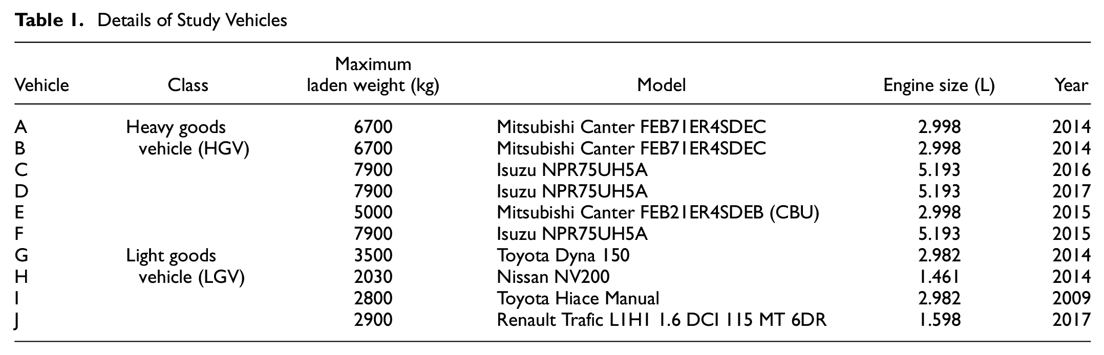
As part of a larger vehicle survey in Singapore, 10 commercial road vehicles were chosen for the study. Six were heavy goods vehicles (HGVs) with a maximum laden weight (MLW) greater than 3.5 tonnes, labeled A to F, while the remaining four were light goods vehicles (LGVs) with an MLW less than or equal to 3.5 tonnes, labeled G to J. Data for vehicle A were collected in 2015, while data for the remaining vehicles were collected in 2018/19. Information on the vehicles’ make and model, MLW, unladen weight (ULW), engine size, and year of manufacture was obtained from the Singapore national vehicle registry ( 25 ). Manufacturer specifications were obtained from online sources or vehicle dealers. These details, shown here in Table 1 and Table S1 in the supplemental material, are key inputs to the three fuel consumption models chosen in this study.

Table 1.

Details of Study Vehicles

Vehicle	Class	Maximum laden weight (kg)	Model	Engine size (L)	Year
A	Heavy goods vehicle (HGV)	6700	Mitsubishi Canter FEB71ER4SDEC	2.998	2014
B		6700	Mitsubishi Canter FEB71ER4SDEC	2.998	2014
C		7900	Isuzu NPR75UH5A	5.193	2016
D		7900	Isuzu NPR75UH5A	5.193	2017
E		5000	Mitsubishi Canter FEB21ER4SDEB (CBU)	2.998	2015
F		7900	Isuzu NPR75UH5A	5.193	2015
G	Light goods vehicle (LGV)	3500	Toyota Dyna 150	2.982	2014
H		2030	Nissan NV200	1.461	2014
I		2800	Toyota Hiace Manual	2.982	2009
J		2900	Renault Trafic L1H1 1.6 DCI 115 MT 6DR	1.598	2017

Model Parameter Settings

Where available, vehicle registry data and manufacturer specifications were used as model inputs. Otherwise, default values for each model were used, depending on which category the vehicles fall under for each model. The three models typically classify vehicles by MLW. For example, vehicle A with an MLW of 6.7 tonnes will fall under the “Rigid <=7,5t” in COPERT 4, and fall under “sourceTypeID 52” (single unit short-haul trucks) in MOVES ( 24 ). Unless stated otherwise, all vehicles were assumed to be operating at half capacity—the midpoint between ULW and MLW. Table S3 in the supplemental material details the relevant parameter settings for each of the three models.

Standardized Drive Cycle

The models were first applied to the NEDC to provide a baseline comparison between them. This drive cycle is also used in Singapore to record CO₂ emissions rates and fuel consumption for passenger cars and LGVs ( 25 ). For each of the 10 study vehicles, the three models were applied to this common speed-time trace ( 7 ). The payload was set to the vehicle’s reference mass (ULW+100 kg), and a road grade of zero (flat road) was used for the model runs. Fuel consumption data is available for vehicles G to J as they are included in Singapore’s fuel economy testing program.

Real-World Activity Data

Data Collection and Processing

A GPS/OBD data logger on each vehicle provided synchronous data at up to 1 Hz frequency. Data for each vehicle were collected for at least five working days. Table S4 and Figure S2 in the supplemental material detail the data collection period and equipment used for the 10 study vehicles. GPS instantaneous speed was filtered ( 26 ) to correct for common errors associated with GPS data. Additionally, the loggers were connected to the engine ignition switch, which allowed engine idling to be easily determined. The logger also collects OBD data via the vehicle’s OBD port. Most OBD parameters were unavailable, but calculated engine load (PID 04) and mass air flow (PID 10) were available, allowing fuel flow to be calculated with Equation 1 ( 4 , 5 ):

Fuel Rate = \frac{\frac{MAF}{1000} \times \frac{Load}{100}}{η \times ρ}

(1)

with $Fuel Rate$ in L/s, $MAF$ (mass air flow) in g/s, $Load$ (calculated engine load) in percentage, $η$ (stoichiometric ratio) dimensionless, and $ρ$ (fuel density) in kg/L. Engine load and mass air flow rates can provide good estimates of fuel flow with calibration ( 4 ). Typical values of $η = 14.5$ and $ρ = 0.832$ kg/L for diesel were used.

Finally, payload information was obtained via a truck driver activity survey conducted using the Future Mobility Sensing survey platform ( 27 ), where the driver provided information on the activity conducted at the stop, and the volume and type of goods picked up or delivered, if applicable. Six vehicles had valid payload information while the remaining four vehicles either did not take part in the survey, had poor or insufficient data, or lacked responses during the time period with GPS/OBD data.

Road grade has a considerable effect on vehicle fuel consumption ( 14 , 28 ). In this study, elevation data was obtained from a DEM of one-arcsecond resolution ( 29 ). Given a series of GPS points from a vehicle, the elevation of each point was obtained by looking up the corresponding coordinates in the processed DEM. The elevations were then filtered using a multi-step elevation filtration routine ( 30 ).

With GPS data and fuel flow from the OBD, the method of space-time path segments (STPS) was used in the subsequent analysis. STPS are “line segments between consecutive track points” ( 11 , 12 ) where activities and attributes are assigned to each path segment. In this study, each STPS contains information on the vehicle’s previous and future locations, speed, engine status, and road grade. The distance traveled in the STPS was calculated based on the distance between successive location coordinates in the STPS, while the length of time spent in the STPS was calculated by taking the time difference of successive timestamps.

Finally, the three models were applied using the data structure of the STPS and the fuel used during each STPS was obtained.

Choice of a Symmetric Evaluation Metric

After applying each model to the 10 study vehicles, the estimated and actual fuel used from OBD data is aggregated at the trip level, where a trip is defined as an engine on–off cycle. The mean percentage error and mean absolute percentage error (MAPE) are commonly used to evaluate the bias and accuracy of models, but these metrics face the issue of an asymmetric distribution ( 21 ). Overestimations are penalized more heavily, which causes under-estimating models to appear to perform better. The log accuracy ratio addresses the problem of asymmetry and outperforms MAPE when the data is heteroskedastic ( 31 ). This heteroskedasticity is applicable when evaluating fuel use estimates at the trip level, as model errors building up during the trip can cause the magnitude of the errors to increase as the trip gets longer. Morley et al. ( 32 ) built on the log accuracy ratio to create two new metrics: the median symmetric accuracy (MSA) (Equation 2) and the symmetric signed percentage bias (SSPB) (Equation 3).

\begin{matrix} M S A = [\exp {m e d i a n_{i} (| \log (\frac{\hat{y_{i}}}{y_{i}}) |)} - 1] \times 100 % \end{matrix}

(2)

\begin{matrix} S S P B = s i g n (m e d i a n_{i} (\log (\frac{\hat{y_{i}}}{y_{i}}))) \times [\exp {| m e d i a n_{i} (\log (\frac{\hat{y_{i}}}{y_{i}})) |} - 1] \times 100 % \end{matrix}

(3)

where, in the context of trip-level fuel use, $\hat{y_{i}}$ and $y_{i}$ are the estimated and actual fuel use respectively of a particular trip $i$ out of the set of all $n$ trips.

Both metrics are symmetrical in that switching the estimated $(\hat{y_{i}})$ and actual $(y_{i})$ values gives the same output. The median function also makes both indicators robust. The MSA outputs values $[0, \infty)$ , where smaller values indicate higher accuracy. On the other hand, the SSPB gives information on the direction and magnitude of bias. The SSPB outputs values $(- \infty, \infty)$ . Negative values indicate underestimation while positive values indicate overestimation. For each model and vehicle, the MSA and SSPB were calculated over each trip $i$ that was taken. The resulting MSAs and SSPBs are then used to evaluate the performance of each model.

Adding Median Idle Fuel Rates and Payload Information

To test the improvements of adding engine data in estimating fuel use, the median idle fuel rate obtained from OBD data is used in the three models. Incorporating idle fuel rates indirectly accounts for more factors like engine capacity, idling engine speed, vehicle age, and accessory use ( 33 , 34 ). The idling phase is also more stable than the acceleration or cruise phases, which are influenced by more factors such as traffic conditions and driver behavior.

For COPERT 4 and SIDRA TRIP, the idle fuel rate is directly replaced with the observed median idle fuel rate. For MOVES, the energy consumption rate of the idling operating mode bin (‘opMode 1’) is altered to match the observed median idle fuel rate. Table S5 in the supplemental material details the observed median idle fuel rates for each vehicle and the altered model parameters as well as the model defaults for MOVES.

Payload information is incorporated by converting the responses in the driver activity survey into vehicle masses which are the inputs to each fuel consumption model. Pickup and delivery quantities were reported as either “multiple pallets” or volumes such as “100 × 100 × 100 cm.” In the absence of the actual weight of the cargo, the vehicles are assumed to be fully loaded to their MLW when picking up goods, and to distribute the payload evenly as they visit each delivery location along the tour, eventually being empty (ULW) at the end of the tour. Table S6 in the supplemental material provides more details of the type and quantity of goods picked up and delivered.

This variation in payload (and thus vehicle mass) along the route is implemented in different ways according to the features of each fuel consumption model. For COPERT 4, separate coefficients are provided according to the different loading fractions (0, 0.5, and 1.0). For SIDRA TRIP and MOVES, vehicle mass is altered directly.

To determine if the addition of median idle fuel rates from the OBD and payload information made a statistically significant difference to the estimated fuel use, a Fisher sign test was conducted for the most accurate model (SIDRA TRIP) in the context studied. The sign test was conducted in a pairwise fashion between the three levels of information: GPS+OBD versus GPS only, and GPS + OBD + Payload versus GPS + OBD. For each pair, the estimated fuel used for each trip for one level of information was subtracted from the corresponding trip with another level of information. The null hypothesis was that the median of the differences is zero.

Results and Discussion

Fuel Use Based on Standardized Drive Cycle

Of the three models, COPERT 4 generally reports an estimated fuel use of between 1 and 2 L across all 10 vehicles (Figure 1). On the other hand, SIDRA TRIP and MOVES tend to report higher estimates for vehicles A to F of about 3.3 L and also report notably similar estimates within about 0.1 L of each other.

Figure 1.

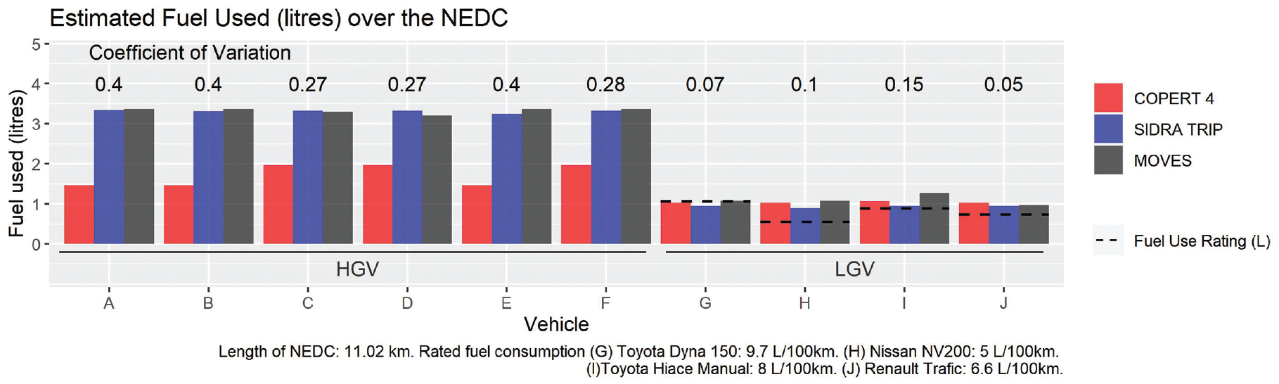
Estimated fuel used (L) for different vehicles over the New European Driving Cycle (NEDC) using COPERT 4, MOVES, and SIDRA TRIP.

The coefficient of variation (CoV) is used as a measure of how well the fuel use estimates agree across the three models. It is defined as the standard deviation of the fuel use estimates from the three models divided by the mean. A lower CoV indicates better agreement between the models. CoV is lowest for vehicles G to J (LGVs) and is the highest for vehicles A to F (HGVs), with vehicles A, B, and E having the highest CoV of 0.4. There is generally good agreement between the models for vehicles G to J and the fuel estimates are also reasonably close to the known fuel use ratings. For example, the estimated fuel use from MOVES was just 0.01 L more than the fuel use rating for vehicle G.

The results shed light on the characteristics of each model. COPERT 4 estimates identical fuel use for the vehicle groups A-B-E, C-D-F, and G-H-J. This is because these vehicle groups are in the same COPERT 4 segment and thus share the same coefficients. Vehicles G to J have identical COPERT 4 coefficients, but vehicle I has a different fuel use estimate because it is a Euro 4 vehicle while the rest of the vehicles are Euro 5. MOVES estimates slightly lower fuel use for vehicle D (3.21 L) compared with vehicle C (3.31 L). This is because vehicle D is one year newer than vehicle C. Additionally, the highly similar estimates from SIDRA TRIP and MOVES for vehicles A to F might be explained by the power-based nature of the two models, in contrast to COPERT 4 which is an average speed model.

These results show that when models are used with default settings, fuel use estimates from the models might not be in good agreement, especially for HGVs, even though identical activity data from a standard drive cycle were used.

Fuel Use Based on Real-World Activity Data

Observing the performance of each model at its original settings with GPS data only (Figure 2), SIDRA TRIP had the least error with the lowest average magnitude of SSPB (32.9%) while results for MOVES had the highest error (49.93%). MOVES overestimated all vehicles (except vehicle C), with the most severe overestimation for vehicle E. COPERT 4 and SIDRA TRIP exhibited more moderate behavior, over-estimating some vehicles and under-estimating others, although COPERT 4 performed slightly worse than SIDRA TRIP on average. Figure S3 in the supplemental material shows model performance according to MSA.

Figure 2.

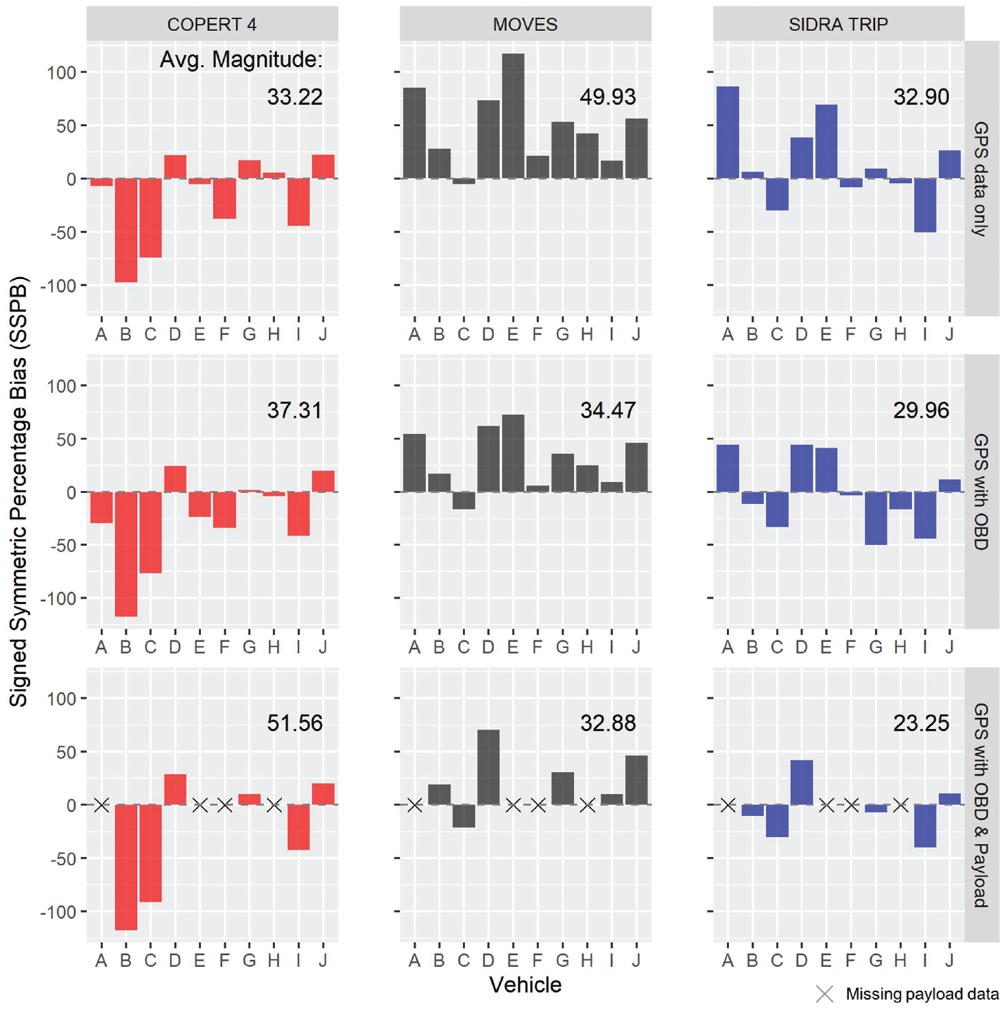
Accuracy of models per vehicle and level of information. Model performance is measured by signed symmetric percentage bias (SSPB) where values closer to zero indicate higher accuracy and positive and negative values denote the direction of bias. The rows show results for the original model with global positioning system (GPS) data only (top), after using median idle fuel rates from the on-board diagnostics (OBD) (middle), and after adding payload information (bottom).

A one-way analysis of variance (ANOVA) was conducted with the null hypothesis that the average MSA was identical for each model at a particular level of information. Insufficient evidence was found to reject the null hypothesis ( $p > 0.05$ ), indicating that the average MSA was not significantly different between each model. This is accounted for by the wide range of model accuracies observed across the 10 vehicles, despite best attempts to account fully for individual vehicle characteristics. While the insignificant difference in average accuracy between the models might suggest that the three models can be used interchangeably, this result should be interpreted with caution because of the small sample size of 10 vehicles.

Across all levels of information, SIDRA TRIP had the lowest average magnitude of error out of all three models, followed closely by COPERT 4 and MOVES. When comparing across the levels of information, the model performance improves (average magnitude of SSPB decreases) consistently for SIDRA TRIP and MOVES as median idle fuel rates from OBD and payload information are added. This is in contrast to COPERT 4, where model performance was observed to deteriorate steadily as more information was added. These findings suggest that additional information does not necessarily lead to improved model performance. Future attempts at improving fuel estimates by incorporating new data sources should conduct evaluations on a case-by-case basis.

When comparing the default idle fuel rates for each model with the observed median idle fuel rate from OBD data (Figure 3), MOVES tends to have higher default idle fuel rates, which would explain the overestimations of MOVES in Figure 2. While SIDRA TRIP only provides two sets of default idle fuel rates—one for LGVs and another for HGVs—the default rates are generally closer to the observed rates compared with MOVES. As default idle fuel rates from SIDRA TRIP were used for COPERT 4, the different behavior of COPERT 4 and SIDRA TRIP when median idle fuel rates from OBD were added implies that the differences in the models are accounted for by the non-idle phases such as acceleration or cruising.

Figure 3.

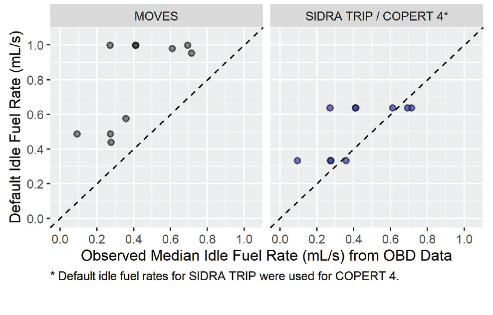
Comparison of default and observed median idle fuel rates (mL/s).

These results show that while it is feasible to obtain fuel use estimates from real-world GPS data using default parameters in each of the three models, these estimates can vary considerably between both models and individual vehicles. Furthermore, the performance of all three models was observed to behave differently when additional information from OBD and payload data were added. The variation in fuel use estimates was also observed in the earlier example of the standardized drive cycle, where the fuel use estimates were not in good agreement, with vehicles G to J being the exception. However, it should be noted that SIDRA TRIP and MOVES were observed to be in agreement with similar results in both the standardized drive cycle and real-world data.

The choice of metric is critical, especially when attempting to pick the most suitable model based on model accuracy. When evaluated with SSPB, SIDRA TRIP had the lowest average magnitude of error across all levels of information (Figure 2). However, when evaluated with the commonly used MAPE, COPERT 4 emerged as the model with the lowest average error across all vehicles when used at its original settings (59.11%) (Figure S4 in supplemental material). As discussed previously, this is a consequence of MAPE penalizing overestimations more heavily and causing under-estimating models (in this case, COPERT 4) to appear to perform better. Therefore, the choice of an evaluation metric for model accuracy is critical and future studies should consider the limitations of various evaluation metrics in model selection.

Further analysis was conducted on SIDRA TRIP to determine if the additional OBD and payload information produced a statistically significant difference in the estimated fuel use. The pair “GPS + OBD versus GPS only” has statistically significant differences for all 10 vehicles, while for the other pair “GPS + OBD +Payload versus GPS + OBD,” only three of the six vehicles had a statistically significant difference (Figure 4). Plotting the percentage differences between the observed median idle fuel rates and the default values used for each vehicle (blue diamonds) shows the strong influence of median fuel rates on the resulting change in estimated fuel use. These results show that the addition of median idle fuel rates from the OBD to SIDRA TRIP leads to significant differences in the estimated fuel used, and the addition of payload information has limited effect on the estimated fuel used. This may imply that, given limited resources in data collection, obtaining median idle fuel rates from OBD data would be a more worthwhile investment in improving fuel use estimates than obtaining vehicle payload information.

Figure 4.

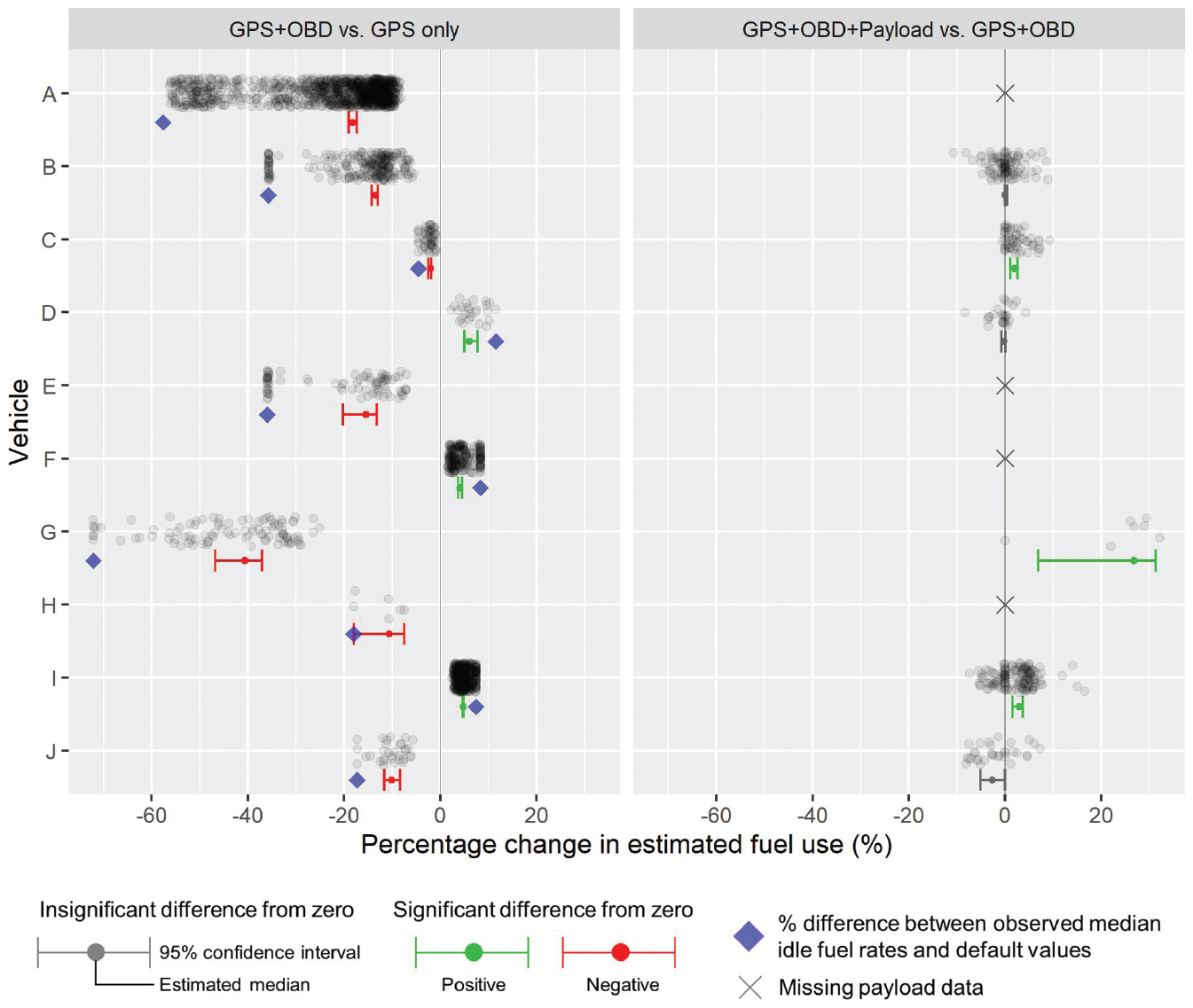
Results from a pairwise Fisher sign test for SIDRA TRIP between the original model settings with global positioning system (GPS) data only, with median idle fuel rate from the on-board diagnostics (GPS + OBD), and with additional payload information (GPS + OBD + Payload).

The results obtained in Figure 4 could arise from the unique activity patterns of each vehicle, which then affects the relative importance of median idle fuel rates or payload information in estimating fuel use. For example, observed idle fuel rates could be more beneficial for a vehicle that spends more time idling. On the other hand, payload information could be more useful for a vehicle that experiences more acceleration events (such as those arising from having multiple delivery locations or being in traffic congestion) and long cruising segments.

Another contributing factor could be the quality of information used in this study. While the real-world variation in vehicle mass was accounted for by incorporating payload information from a truck driver activity survey, the quality of the payload information could be improved further. As the driver responses for the quantity of goods handled were “multiple pallets,” large assumptions had to be made to convert the driver responses into payload mass. The assumption that the vehicles would be loaded to their MLW might not be realistic as commercial road vehicles in urban areas such as Singapore are likely to have lower loading factors. For example, vans (LGVs) in London were found to have an average load factor of 38% ( 35 ). Making this assumption artificially increases the variation in vehicle mass about its route and could lead to higher fuel use estimates.

Fuel use estimates are expected to improve with better quality payload information, which can be attained by installing on-board weighing systems on each vehicle to provide measurements of vehicle mass along the vehicle’s route. Typically used for weight compliance, such systems can remove judgment errors from drivers visually estimating the quantity of cargo handled and reduce the survey burden on the drivers, which contributed to a considerable dropout rate (45.20%) for the driver activity survey ( 36 ).

Conclusion

Using real-world data of GPS, OBD, and payload from 10 commercial road vehicles, this study compared the accuracy of fuel use estimates from three fuel consumption/emission models under the constraint of limited data for calibration. When applied to a standardized drive cycle, the three models provided fuel use estimates close to the published fuel use ratings for LGVs, but fuel use estimates for HGVs had greater variation. With real-world data from commercial road vehicles used in Singapore, SIDRA TRIP was found to be the most accurate of the three models, suggesting its suitability when evaluated in the context of this study. The addition of median idle fuel rates from OBD data and payload information led to consistent performance improvements for SIDRA TRIP and MOVES, but did not improve model performance for COPERT 4. Finally, further analyses showed that the addition of median idle fuel rates from OBD made a significant difference to fuel use estimates, while the addition of payload information did not.

By taking on the role of the analyst with limited data and resources to develop new fuel consumption/emission models or calibrate existing ones, this contribution to the literature offers a method of comparing fuel consumption/emission models so that others may make well-informed choices when applying models on other use cases and perform similar evaluations in their unique situations. Model comparisons can also be made in the context of evaluating the effects of different control strategies for reducing fuel consumption and emissions, which is of particular interest to analysts who rely on such models for decision making. The findings of this study arise from a small sample of just 10 commercial road vehicles in Singapore. Thus, more work is required in establishing and generalizing the limits to which existing models can be applied to different contexts, especially in contexts where tight data constraints limit the extent of calibration. Beyond idle fuel rates and payload information, a comprehensive uncertainty and sensitivity analysis across all parts of the modeling chain, such as input data and model parameters, could unravel nuances in model structure and behavior, allowing for more robust conclusions on model performance.

A novel symmetric evaluation metric was also used to compare the models which overcame the limitations of the more commonly used MAPE metric. Through the process of implementing each model, the study provides a framework for and demonstrates the feasibility of estimating fuel use from GPS data, which can potentially be applied at larger scales. Finally, the study shows how payload variation can be accounted for in estimating fuel use by using responses from a truck driver activity survey.

While the addition of median idle fuel rates from the OBD had a significant effect on the estimated fuel use compared with the addition of payload information, OBD data collection on a larger scale might face issues with installation and incur significant costs, in addition to privacy concerns. Using the tools of value of information and sensitivity analysis, future work could evaluate the trade-offs between the costs of extra data collection and the benefits of better fuel use estimates.

Future work could also extend the study to other exhaust pollutants which might involve the use of more complex models. Furthermore, with recent developments in large-scale, open data sets of vehicle activity ( 1 ), this study can be extended to provide a more rigorous evaluation of fuel consumption models, potentially including future vehicle technologies into the mix.

Supplemental Material

sj-pdf-1-trr-10.1177_03611981211007478 – Supplemental material for Comparing Commercial Vehicle Fuel Consumption Models using Real-World Data under Calibration Constraints

Supplemental material, sj-pdf-1-trr-10.1177_03611981211007478 for Comparing Commercial Vehicle Fuel Consumption Models using Real-World Data under Calibration Constraints by Lih Wei Yeow and Lynette Cheah in Transportation Research Record

Footnotes

Acknowledgements

The authors would like to thank Dr Rahmi Akçelik at SIDRA Solutions for providing updated SIDRA TRIP parameters for heavy vehicles, and Professor Randall Guensler and Dr Haobing Liu at the Georgia Institute of Technology for generously providing access and assistance with MOVES-Matrix.

Author Contributions

The authors confirm contribution to the paper as follows: study conception and design: L. W. Yeow, L. Cheah; data collection: L. Cheah; analysis and interpretation of results: L. W. Yeow, L. Cheah; draft manuscript preparation: L. W. Yeow, L. Cheah. All authors reviewed the results and approved the final version of the manuscript.

Declaration of Conflicting Interests

The author(s) declared no potential conflicts of interest with respect to the research, authorship, and/or publication of this article.

Funding

The author(s) received no financial support for the research, authorship, and/or publication of this article.

Data Accessibility Statement

The data used in the analysis, such as GPS and OBD data, relevant responses from the driver activity survey, and trip-level fuel use (recorded and estimated) are available in the Figshare repository at . Latitude and longitude coordinates have been removed for privacy.

Supplemental Material

Supplemental material for this article is available online.

References

G. S.

Leblanc

D. J.

Peng

Vehicle Energy Dataset (VED), A Large-Scale Dataset for Vehicle Energy Consumption Research. arXiv: Physics and Society, 2019.

Yang

Zhang

Niu

Wang

Zhang

K. M.

High-Resolution Mapping of Vehicle Emissions of Atmospheric Pollutants Based on Large-Scale, Real-World Traffic Datasets. Atmospheric Chemistry and Physics, Vol. 19, No. 13, 2019, pp. 8831–8843.

Sharpe

Muncrief

Literature Review: Real-World Fuel Consumption of Heavy-Duty Vehicles in the United States, China, and the European Union. International Council on Clean Transportation, Washington, D.C., 2015.

Alessandrini

Filippi

Ortenzi

Consumption Calculation of Vehicles Using OBD Data. Proc., 2012 International Emission Inventory Conference, Tampa, Florida, 2012.

Ribeiro

Rodrigues

J. G. P.

Aguiar

Mining Geographic Data for Fuel Consumption Estimation. Proc., 16th International IEEE Conference on Intelligent Transportation Systems (ITSC 2013), The Hague, Netherlands, 2013, pp. 124–129.

Kousoulidou

Fontaras

Ntziachristos

Bonnel

Samaras

Use of Portable Emissions Measurement System (PEMS) for the Development of Passenger Car Emission Factors and Validation of Existing Models. Atmospheric Environment, Vol. 64, 2013, pp. 329–338.

United Nations. UN Regulation No. 101—Rev.3: Uniform provisions concerning the approval of passenger cars powered by an internal combustion engine only, or powered by a hybrid electric power train with regard to the measurement of the emission of carbon dioxide and fuel consumption and/or the measurement of electric energy consumption and electric range, and of categories M1 and N1 vehicles powered by an electric power train only with regard to the measurement of electric energy consumption and electric range, 2013.

Zhou

Jin

Wang

A Review of Vehicle Fuel Consumption Models to Evaluate Eco-Driving and Eco-Routing. Transportation Research Part D: Transport and Environment, Vol. 49, 2016, pp. 203–218.

Turton

Fuel Consumption Measurements – Carbon Balance vs. Flow Meter. U.S. Environmental Protection Agency, Washington, D.C., 1979.

10.

Smit

Dia

Morawska

Road Traffic Emission and Fuel Consumption Modelling: Trends, New Developments and Future Challenges. In S. Demidov and J. Bonnet (Eds.), Traffic Related Air Pollution and Internal Combustion Engines, Nova Science Publishers, Hauppauge, NY, 2009, pp. 29–68.

11.

Kan

Tang

Kwan

M.-P.

Ren

Liu

Pei

Liu

Deng

Fine-Grained Analysis on Fuel-Consumption and Emission from Vehicles Trace. Journal of Cleaner Production, Vol. 203, 2018, pp. 340–352.

12.

Kan

Tang

Kwan

M.-P.

Zhang

Estimating Vehicle Fuel Consumption and Emissions Using GPS Big Data. International Journal of Environmental Research and Public Health, Vol. 15, No. 4, 2018, p. 566.

13.

Demir

Bektaş

Laporte

A Comparative Analysis of Several Vehicle Emission Models for Road Freight Transportation. Transportation Research Part D: Transport and Environment, Vol. 16, No. 5, 2011, pp. 347–357.

14.

Andersen

Torp

Accurate Fuel Estimates Using CAN Bus Data and 3D Maps. Proc., 2018 19th IEEE International Conference on Mobile Data Management (MDM), Aalborg, Denmark, 2018, pp. 257–265.

15.

Guensler

Liu

Akanser

Kim

Hunter

M. P.

Rodgers

M. O.

Energy Consumption and Emissions Modeling of Individual Vehicles. Transportation Research Record, 2017. 2627: 93–102.

16.

Smit

Ntziachristos

COPERT Australia: A New Software to Estimate Vehicle Emissions in Australia. Proc., ATRF Conference, Brisbane, Australia, 2013, pp. 2–4.

17.

Rakha

H. A.

Ahn

Moran

Saerens

Bulck

E. V. D.

Virginia Tech Comprehensive Power-Based Fuel Consumption Model: Model Development and Testing. Transportation Research Part D: Transport and Environment, Vol. 16, No. 7, 2011, pp. 492–503.

18.

Wang

Rakha

H. A.

Fuel Consumption Model for Heavy Duty Diesel Trucks: Model Development and Testing. Transportation Research Part D: Transport and Environment, Vol. 55, 2017, pp. 127–141.

19.

Rakha

Ahn

Trani

Comparison of MOBILE5a, MOBILE6, VT-MICRO, and CMEM Models for Estimating Hot-Stabilized Light-Duty Gasoline Vehicle Emissions. Canadian Journal of Civil Engineering, Vol. 30, No. 6, 2003, pp. 1010–1021.

20.

Guo

Yang

Jensen

C. S.

Kaul

EcoMark: Evaluating Models of Vehicular Environmental Impact. Proc., 20th International Conference on Advances in Geographic Information Systems, Redondo Beach, CA, 2012.

21.

Smit

Ntziachristos

Boulter

Validation of Road Vehicle and Traffic Emission Models: A Review and Meta-Analysis. Atmospheric Environment, Vol. 44, No. 25, 2010, pp. 2943–2953.

22.

Ntziachristos

Samaras

1.A.3.b.i–iv Road Transport. In EMEP/EEA Air Pollution Emission Inventory Guidebook 2016, Publications Office of the European Union, Luxembourg, 2016.

23.

Akçelik

Smit

Besley

Recalibration of a Vehicle Power Model for Fuel and Emission Estimation and Its Effect on Assessment of Alternative Intersection Treatments. Proc., TRB 4th International Conference on Roundabouts, Seattle, WA, 2014, pp. 16–18.

24.

Population and Activity of On-road Vehicles in MOVES2014, U.S. Environmental Protection Agency, Washington, D.C., 2015.

25.

Land Transport Authority. Procedures on Importation and Registration of a Goods Vehicle in Singapore, Singapore, 2017.

26.

Duran

Earleywine

GPS Data Filtration Method for Drive Cycle Analysis Applications, SAE Technical Paper 2012-01-0743, SAE International, Warrendale, PA, 2012.

27.

Teo

Cheah

Lee

Marzano

Santos

Azevedo

Zhao

Ben-Akiva

An Integrated Sensing-Based Urban Freight Data Collection Framework: Methodology and Pilot Projects in Singapore. Proc., URBE Conference, Rome, 2015.

28.

Wood

Burton

Duran

Gonder

Contribution of Road Grade to the Energy Use of Modern Automobiles Across Large Datasets of Real-World Drive Cycles. National Renewable Energy Lab. (NREL), Golden, CO, 2014.

29.

Magrath

Brady

Evaluating Different Methods for Determining Road Grade Best Suited to Advanced Bus Transportation Systems. Proc., 2017 IEEE International Conference on Service Operations and Logistics, and Informatics (SOLI), Bari, Italy, 2017, pp. 108–113.

30.

Wood

Burton

Duran

Gonder

Appending High-Resolution Elevation Data to GPS Speed Traces for Vehicle Energy Modeling and Simulation. National Renewable Energy Lab. (NREL), Golden, CO, 2014.

31.

Tofallis

A Better Measure of Relative Prediction Accuracy for Model Selection and Model Estimation. Journal of the Operational Research Society, Vol. 66, No. 8, 2015, pp. 1352–1362.

32.

Morley

S. K.

Brito

T. V.

Welling

D. T.

Measures of Model Performance Based on the Log Accuracy Ratio. Space Weather, Vol. 16, No. 1, 2018, pp. 69–88.

33.

Brodrick

C. J.

Dwyer

H. A.

Farshchi

Harris

D. B.

King

F. G.

Jr.

Effects of Engine Speed and Accessory Load on Idling Emissions from Heavy-Duty Diesel Truck Engines. Journal of the Air & Waste Management Association, Vol. 52, No. 9, 2002, pp. 1026–1031.

34.

Lutsey

Brodrick

C.-J.

Sperling

Oglesby

Heavy-Duty Truck Idling Characteristics: Results from a Nationwide Truck Survey. Transportation Research Record: Journal of the Transportation Research Board, 2004. 1880: 29–38.

35.

Transport for London. Roads Task Force: Technical Note 5. What Are the Main Trends and Developments Affecting Van Traffic in London?Transport for London, London, UK, 2013.

36.

Alho

A. R.

You

Cheah

Zhao

Ben-Akiva

Next-Generation Freight Vehicle Surveys by Supplementing Truck GPS Tracking with a Driver Activity Survey: Account and Insights. Proc., 21st IEEE International Conference on Intelligent Transportation Systems (ITSC), Maui, Hawaii, USA, 2018.

Supplementary Material

Please find the following supplemental material available below.

For Open Access articles published under a Creative Commons License, all supplemental material carries the same license as the article it is associated with.

For non-Open Access articles published, all supplemental material carries a non-exclusive license, and permission requests for re-use of supplemental material or any part of supplemental material shall be sent directly to the copyright owner as specified in the copyright notice associated with the article.

0.00 MB

1.09 MB