
Abstract
Microscopic simulation models have been widely used as tools to investigate the operation of traffic systems and different intelligent transportation systems applications. The fidelity of microscopic simulation tools depends on the driving behavior models that they implement. However, current models commonly do not consider human-related factors, such as distraction. The potential for distraction while driving has increased rapidly with the availability of smartphones and other connected and infotainment devices. Thus, an understanding of the impact of distraction on driving behavior is essential to improve the realism of microscopic traffic tools and support safety and other applications that are sensitive to it. This study focuses on car-following behavior in the context of distracting activities. The parameters of the well-known GM and intelligent driver models are estimated under various distraction scenarios using data collected with an experiment conducted in a driving simulator. The estimation results show that drivers are less sensitive to their leaders while talking on the phone and especially while texting. The estimated models are implemented in a microscopic traffic simulation model. The average speed, coefficient of variation of speed, acceleration noise and acceleration and deceleration time fractions were used as measures of performance indicating traffic flow and safety implications. The simulation results show deterioration of traffic flow with texting and to some extent talking on the phone: average speeds are lower and the coefficient of variation of speeds are higher. Further experimentation with varying fractions of texting drivers showed similar trends.
There is no universally agreed definition of driver distraction. The definitions in the literature vary. One is: “driver distraction occurs when a driver is delayed in the recognition of information needed to safely accomplish the driving task because some event, activity, object or person within or outside the vehicle compelled or tended to induce the driver’s shifting attention away from the driving task” ( 1 ). Alternatively, driver distraction is defined as: “a shift in attention away from stimuli critical to safe driving toward stimuli that are not related to safe driving” ( 2 ). Driver distraction, in all its forms, has been found to affect driver performance, especially at the operational and tactical levels (3, 4). At these levels, drivers are required to make continuous and timely decisions, within fractions of seconds, to safely control their vehicles ( 5 ). Thus, secondary tasks, even for short durations, and especially those that involve visual, auditory, biomechanical (physical) and cognitive distractions, might lead to failures in drivers’ performance and consequently to crashes ( 6 ). Visual distraction, such as reading a text message, which causes drivers to take their eyes off the road, was found to involve substantial increase in crash risk since the driving environment may change rapidly ( 7 ). Auditory distraction occurs when drivers focus their attention on auditory signals rather than on the road environment, such as when listening to the radio or music. Biomechanical or physical distraction occurs when drivers remove one or both hands from the steering wheel for extended periods of time to physically manipulate an object. Cognitive distraction occurs when drivers look at the road but fail to see, that is, they do not perceive what they see (8, 9). This happens because secondary tasks compete over the limited central processing resources in the brain. Carsten and Brookhuis ( 10 ) found that when drivers are cognitively distracted, their car-following behavior is impaired, while their lane-keeping performance improved. The latter is a result of a “tunnel vision” effect in which drivers focus their attention on the center of the road. In a driving simulator study, Muhrer and Vollrath ( 11 ) found that cognitive distraction negatively influences the anticipation of the behavior of other drivers, while visual distraction deteriorates the perception and reaction to unexpected events. They found that the minimum time to collision was smaller with visual distraction than with cognitive distraction.
Car-following behavior is one of the main building blocks of microscopic simulation models. It is defined as when the subject vehicle follows the vehicle in front of it (the leader) and reacts to its actions. Gazis et al. ( 12 ) developed the GM model which considers a non-linearity in the effect of the spacing and the subject vehicle speed on the sensitivity of the response to the stimuli, which is the speed difference with respect to the leader. Over the years, many studies followed this line of research, trying to improve the model in different ways, such as suggesting various stimuli and objectives for the driver (e.g., keeping desired spacing or headways, desired speeds, limits on maximum accelerations), differentiating parameters for acceleration and deceleration decisions, and so on. For thorough reviews see Brackstone and McDonald ( 13 ), Toledo ( 14 ), Hamdar ( 15 ), and Treiber and Kesting ( 16 ), among others. Despite the wide range of proposed models, they mostly represent an idealized environment, which does not account for human factors and errors. Saifuzzaman and Zheng ( 17 ) term these “engineering models” and argue that they lack in their inability to capture human factors.
Few studies have dealt with the development of driver models that explicitly incorporate human factors, and specifically distraction. Relevant theoretical behavioral frameworks were proposed by Fuller (18, 19), Hamdar ( 15 ), and Schomig and Metz ( 20 ). Even fewer studies have attempted to translate these theories into car-following specifications. Yang and Peng ( 21 ) and Przybyla et al. ( 22 ) assume that distracted followers maintain their previous speeds rather than react to their leaders. Distraction episodes and their durations are randomly drawn from their assumed distributions. Yang and Peng ( 21 ) also introduce perception errors and time delays in their model, which extends a variant of the GM car-following model. Przybyle et al. ( 22 ) use Newell’s model for car following. Their analysis is focused on crash rates, and so they do not evaluate microscopic level accelerations. Hoogendoorn et al. ( 23 ) incorporate the task capability interface (TCI) model within the intelligent driver model (IDM) car-following model. TCI assumes that driving performance is negatively affected when the task demand is higher than the driver capability. The latter is affected by distraction. In the modified IDM, free flow speeds, desired spacings and maximum accelerations are all affected by the difference between task demand and driver capability. The authors demonstrate the sensitivity of traffic flow to varying TCI measures, but do not discuss how these may be estimated from data. Van Lint et al. ( 24 ) use a similar model within the OpenTrafficSimulation model. They use an assumed distribution for distraction values, which varies both within and between drivers. The distraction value affects desired speeds and reaction times. They also do not show how the parameters of this model may be estimated. Saifuzzaman et al. ( 25 ) apply modifications to the GM and IDM to capture the TCI. In their model task, difficulty is captured by the ratio between task demand and driver capability. Its expression depends on the vehicle’s speed, pacing, desired headway and a risk factor. It affects the maximum acceleration and deceleration in the GM and the desired spacing in the IDM. They estimate the modified model using driving simulator data that was collected with and without distraction. Van Lint and Calvert ( 26 ) present a comprehensive framework, also based on TCI, to incorporate human factors, including distraction, into driving models. In their model, task saturation, which is influenced by distraction, affects various errors that the driver may make. They demonstrate how this framework is incorporated with a version of the IDM and propose functional forms for the various components of the model. They demonstrate their model with an application to distracted driving and show that it produces conceptually plausible results. However, they do not discuss methods and data needs for model estimation.
The approaches described above that explicitly incorporate human factors within driving behavior are conceptually desirable and useful, certainly in the context of driving performance. However, they also have limitations: methods and data to test their functional form and estimate their parameters may be difficult to collect; in application, they may be computationally expensive and require inputs (e.g., on distributions of human traits, frequencies and durations of various types of distractions) that are not readily available. This study focuses on engineering-level car-following behavior in the context of distracting activities. The parameters of the well-known GM and IDM are estimated under various distraction scenarios using data collected in a driving simulator. The best fit estimated models are implemented in a microscopic traffic simulation model. The simulation model is then used in a case study of an urban arterial in Haifa, Israel. The impact of the distracting activities on traffic flow are evaluated using performance measures that are derived from the simulation results.
The rest of this paper is organized as follows: the next section describes the simulator experiment and presents summary statistics for the collected data. Next, the method to estimate the parameters of the car-following models under the various distraction conditions and the estimation results are presented. This is followed by the implementation of the best estimated car-following models within the microscopic traffic Simulation TRANSMODELER and results of a case study to evaluate the effects on traffic flow. Finally, the results are discussed in a conclusion section.
Driving Simulator Experiment
A laboratory experiment using a driving simulator was developed to collect data on driving behavior while undertaking different distracting activities. The simulation scenarios included a two-lane rural highway. Lane and shoulder widths were 3.75 m and 1.5 m, respectively. The sections were designed on a level terrain and with no intersections. The scenarios were designed with daytime and good weather conditions which allowed good visibility. Drivers were instructed to drive as they would normally in the real world. They were told not to pass the vehicle in front. This was also indicated by the markings on the road. Following previous studies (27, 28) drivers were given between 5 and 10 min training to become familiar with the simulator.
A scenario took about 4 min to complete. Each scenario was composed of six sections with different speeds for the vehicle in front of the subject. The leader speed in each section was constant, and different from that of the preceding and following sections. The speed transition from one section to the next was determined by a constant acceleration (or deceleration) rate, which was randomly selected in the range 0.4 to 2.5 m/s2. Four levels of speed ranges were used: 20–40, 40–60, 60–80, and 80–100 km/h. The realized lead speed was drawn from a uniform distribution over the speed range within the specific level. The duration of constant speed sections was 40 s when the speed was in the range of 20 to 80 km/h, and 30 s when the speed was over 80 km/h. Figure 1 shows an example of the leader vehicle speed profile from one of the scenarios in the experiment.
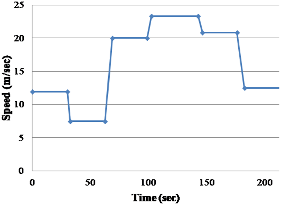
An example of the speed profile of the lead vehicle.
Vehicles in the opposing direction traveled at a constant speed of 70 km/h. In the event that the driver is involved in a crash, for example a rear-end crash with the lead vehicle, the driver hears a sound of crashing, the windshield breaks, and the subject vehicle comes to a full stop. Then, the lead vehicle disappears and the scenario continues from the same point the crash occurs, with a new lead vehicle.
Twenty-four different scenarios were generated. Drivers drove four different scenarios each. In each one of the scenarios, the drivers were engaged in one of four distraction conditions. In all cases the activities took place throughout the driving scenario:
Making a cell phone call (hand-held): drivers received a phone call at the beginning of the scenario and were engaged in a conversation with the experimenter, in which they were asked several general questions.
Sending and receiving text messages: drivers received messages with general questions to their own cell phones and were requested to reply to those messages.
Eating a snack: the participating drivers were requested to eat a snack, such as potato chips, while driving.
No distracting activities (control case): the driver did not have any secondary tasks beside the primary task of driving.
The order of the activities within the experiment was randomly chosen.
The simulator used in this experiment, STISIM ( 29 ), is a fixed-base interactive driving simulator, which has a 60° horizontal and 40° vertical display. The changing alignment and driving scene were projected onto a screen in front of the driver. The simulator updates the images at a rate of 30 frames per second.
Participants were recruited using billboard advertisements at the Technion campus. Participation was voluntary, with screening criteria that the participant holds a driving license and drives on a regular basis. Participants were compensated with a voucher for a coffee shop at a value of about 6 USD. In total, 101 participants (68 males, 33 females) completed the simulator experiment. Their ages ranged from 18 to 57 years (mean = 27.8; standard deviation = 8.3 years). On average the drivers had a driving license for 4 years.
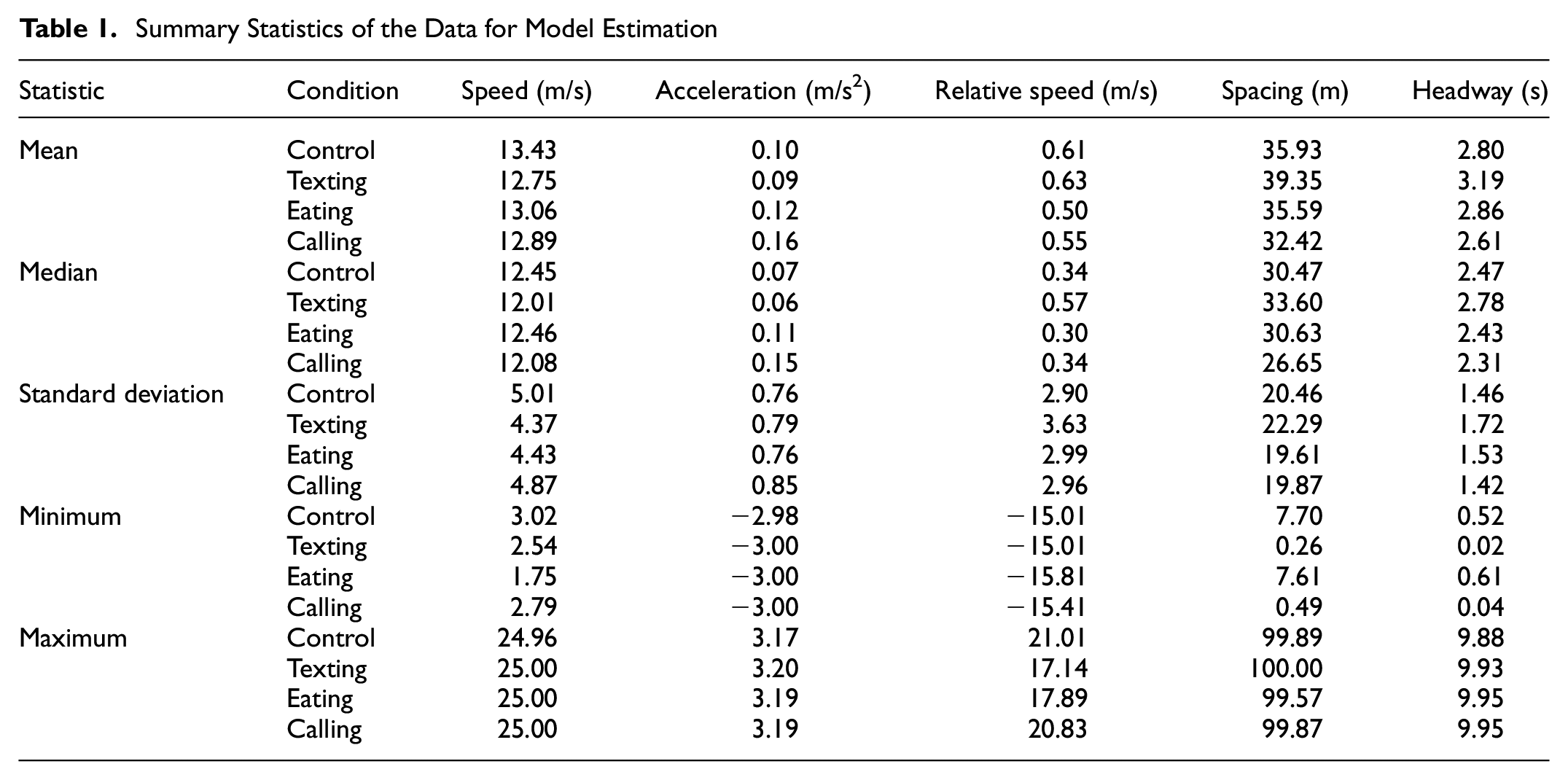
The collected data include observations of the detailed trajectories of individual vehicles in various situations. These include speed and acceleration of the subject vehicle and the leader with resolution of 0.5 s. Only the data of the acceleration and deceleration sections were used to estimate the car-following models. This was done to avoid overfitting of the acceleration functions in the constant speed sections, where control errors the accelerations, which both theoretically and in the data tend to zero. The estimation dataset included a total of 5,610, 4,113, 4,327, and 5,301 observations for the control, texting, eating, and calling scenarios, respectively. Table 1 presents summary statistics for the data with the control and various distraction conditions.
Summary Statistics of the Data for Model Estimation
Car-Following Models
GM Model
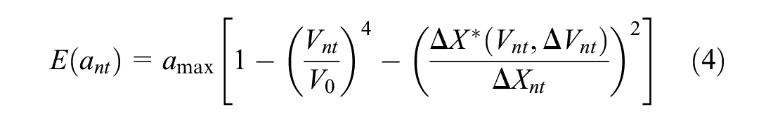
The GM model is based on the sensitivity-stimulus framework, which assumes that the driver reacts to stimuli from the environment. In the GM model, the stimulus is the leader relative speed (the speed of the leader less the speed of the subject vehicle). The sensitivity depends on the vehicle’s speed and the distance between the two vehicles. The original formulation accounts for reaction time, but not for broader heterogeneity in behavior among drivers. The formulation below accounts for serial correlation because of driver-specific terms. Including reaction time in the specification, in addition to driver-specific heterogeneity, may lead to identification issues. Furthermore, microscopic traffic simulation models generally do not explicitly model reaction time. Therefore, it is omitted in the following functional form. However, a nonlinear stimulus is used:

where
The applied acceleration includes the expected value and error terms. It is assumed that the error term is comprised of two components: The first is a driver-specific term that does not vary over time. It captures heterogeneity in the behavior, including indirectly in reaction times. The second is a generic random term:

where
Finally, it is hypothesized that the response to the stimuli is positive (acceleration) for positive leader relative speeds, that is, when the leader is faster than the subject vehicle and negative (deceleration) for negative leader relative speeds. Furthermore, it is asymmetric, with different sets of parameters in the two cases. The acceleration is therefore given by:

where
IDM
The IDM assumes that drivers maintain a safe following distance from the leader and at the same time attain a desired speed
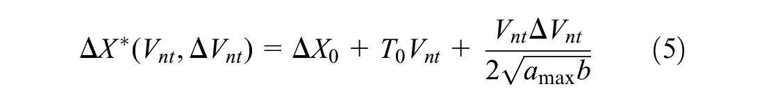
where
In the context of distraction, Hoogendoorn et al. ( 30 ) and Van Lint and Calvert ( 26 ) used the IDM to incorporate mental workload, task demand, and awareness in car-following behavior.
The acceleration that the vehicle applies included individual-specific and generic error terms, introduced in the same way as shown in Equation 2.
Model Estimation
The parameters of both models were estimated using the maximum likelihood method applied on the acceleration observations in trajectory data. For the GM model, the conditional probability density function of the observed accelerations is given by:
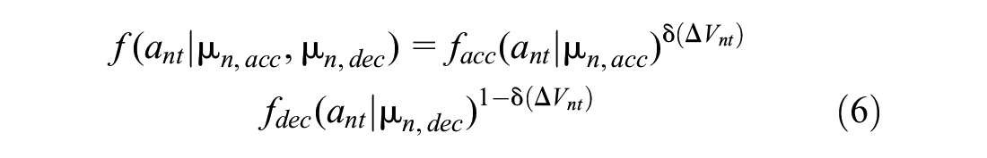
where the subscripts

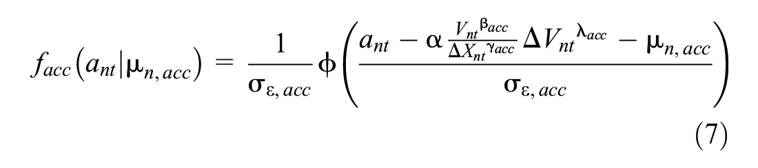
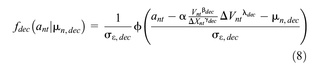
The conditional probability density functions for the acceleration and deceleration regimes are given by:
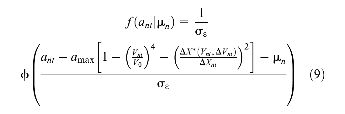
For the IDM, the conditional probability density function of the observed accelerations is given by:
With both models, the conditional probability density for the sequence of
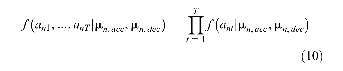
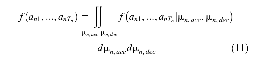
The unconditional joint probabilities of the observations for a driver are given by:
Finally, the likelihood functions are given by:

The model parameters were estimated by maximization of these functions. The unconstrained optimization was done using the maxLik package in R and using the BFGS quasi-Newton optimization method it implements; see Henningsen and Toomet ( 31 ) for details.
Estimation Results
GM Model
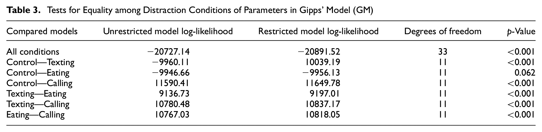
As noted above, separate models were estimated for each of the distraction conditions (control, texting, eating, talking on the phone) that were used in the simulator experiment. The results for the GM models are presented in Table 2. The hypothesis of equality of the parameters among the four conditions was tested using likelihood ratio tests. The results are shown in Table 3. The hypothesis that the parameters are similar for all four conditions is rejected with a p-value less than 0.001. The hypothesis of equality of parameters is rejected also for all pairs of conditions, except the control and eating conditions for which the p-value is 0.062. To illustrate these results and the differences among the conditions, Figures 2 and 3 show the effect on the mean accelerations and decelerations of the changes in the explanatory variables: leader relative speed, spacing and subject’s speed, respectively. In each figure, one of the variables varies while the others are held at their base value. These base values are: relative speed = 5 (or −5) m/s, subject speed =15 m/s, and spacing = 25 m.
Estimation Results of Gipps’ Model (GM)
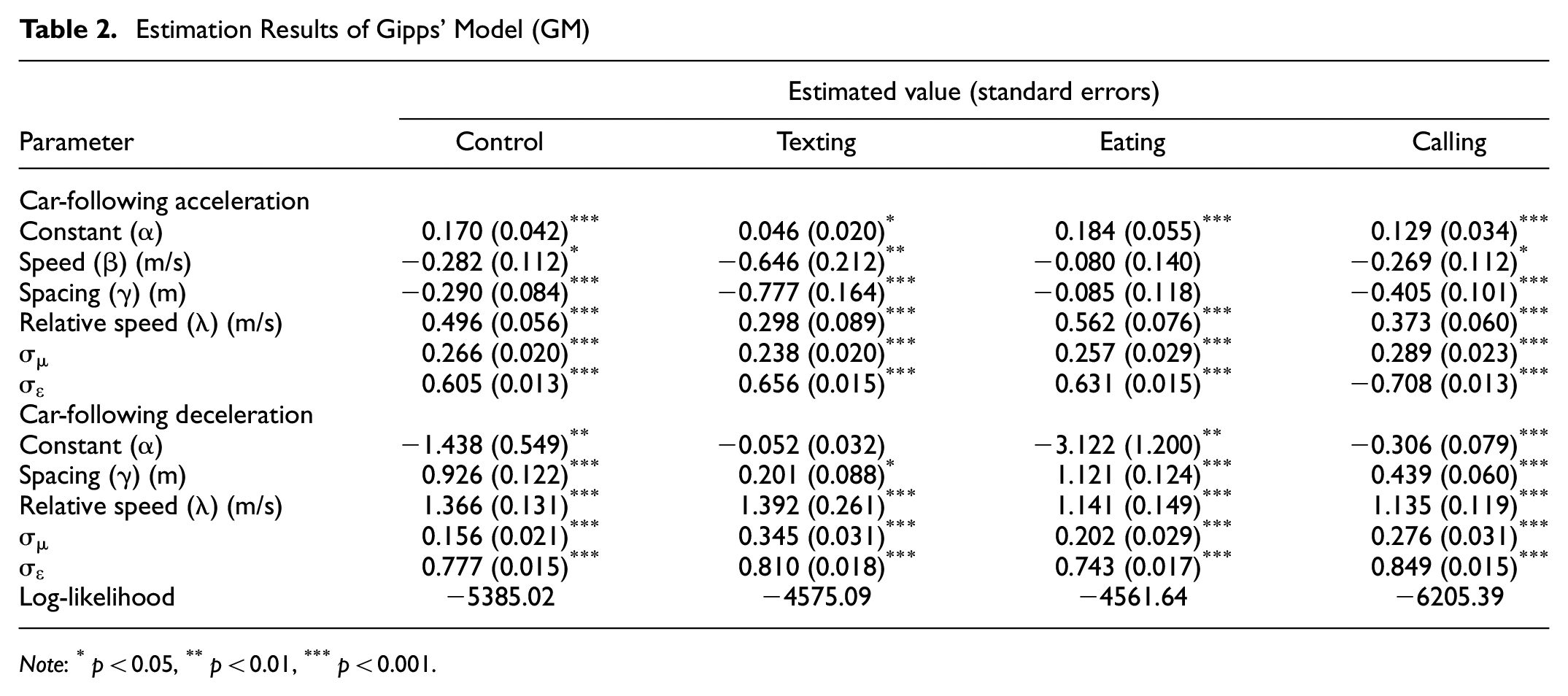
Note: *p < 0.05, **p < 0.01, ***p < 0.001.
Tests for Equality among Distraction Conditions of Parameters in Gipps’ Model (GM)
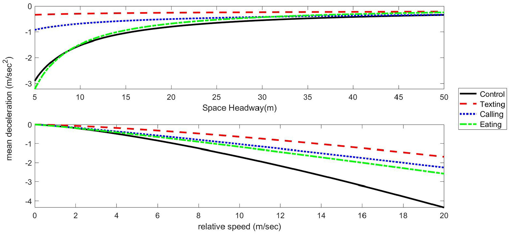
Effects of different variables on mean car-following deceleration in Gipps’ model (GM).
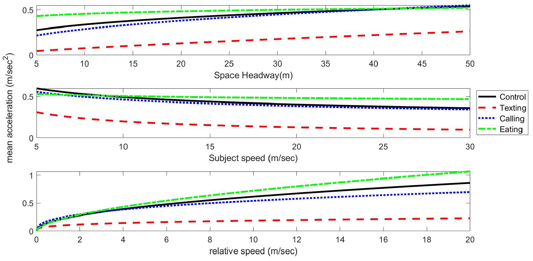
Effects of different variables on mean car-following acceleration in Gipps’ model (GM).
As expected, the constant sensitivity terms (
The parameter associated with the stimulus (relative leader speed) is positive for both acceleration and deceleration. Its magnitude is much larger when it is negative (i.e., the subject is faster) compared with when it is positive (i.e., the leader is faster). This is expected since a negative relative speed stimulus may have safety implications, whereas a positive relative leader speed stimulus only suggests a possible speed advantage to the driver. The GM model assumes that drivers respond to the leader relative speed. This response, as demonstrated in Figures 2 and 3, is much lower in absolute value for texting, compared with the control and two other conditions in both acceleration and deceleration conditions. This may be a result of the visual distraction associated with texting ( 7 ).
The estimated coefficients of the spacing are positive for car-following deceleration and negative for car-following acceleration. For deceleration, this is expected since the underlying safety concern increases when the spacing is smaller, and so drivers would tend to apply stronger decelerations when the spacing is smaller. In the case of acceleration, as the spacing increases, drivers are able to apply strong accelerations. Similar to relative speeds, the effect of this parameter is lower in the texting condition compared with the control, both in acceleration and deceleration. In deceleration, it is also lower in the calling condition. Thus, in these two conditions, drivers are less responsive to the spacing.
The estimated coefficient of the subject’s speed in the acceleration model is negative. Drivers accelerate at a lower rate when their speed is higher. As with the other variables, the sensitivity of the acceleration to the subject’s speed is lower in the texting condition compared with the control and two other conditions. The speed parameter was not significant for deceleration, and therefore was dropped from the specification. This result is consistent with that of Gazis et al. ( 12 ) and Ahmed ( 32 ).
IDM
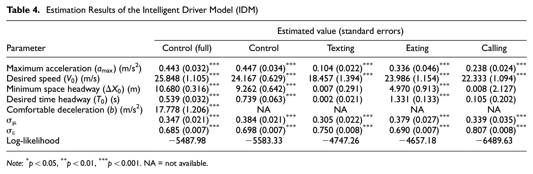
Estimation results of the IDM are presented in a Table 4. In all models, the comfortable deceleration estimate was unrealistically large. This caused the third term in the desired spacing expression to tend to zero. In this case study, this result is reasonable. The term that was removed is relevant in cases when the subject approaches a slower leader. This was not the case in the current experiment design. The term was therefore removed and the models re-estimated without it. For completeness, this paper reports also the results for the full control model with this term. The differences in the estimates of the remaining parameters are small.
Estimation Results of the Intelligent Driver Model (IDM)
Note: *p < 0.05, **p < 0.01, ***p < 0.001. NA = not available.
The overall effects of the various distracting activities are similar to those found with the GM model. The maximum acceleration parameter is lower for the calling and texting conditions compared with the control and eating, indicating a lower level of response to the surroundings. Desired speeds are also lower, which is consistent with the expected impact of the lower attention dedicated to the driving task. With both calling and texting, the minimum spacing and desired headway parameters are very close to zero and statistically insignificant. Thus, the model shows that drivers in these conditions in practice do not respond to the spacing to the leader or to the speed difference. These effects are evident in Figure 4, which shows the effect of spacing and subject’s speed on the mean acceleration. In both texting and calling conditions, the mean acceleration is not affected by the space headway. The effect of speed on the acceleration is also much lower in these two conditions compared with the control and eating conditions.
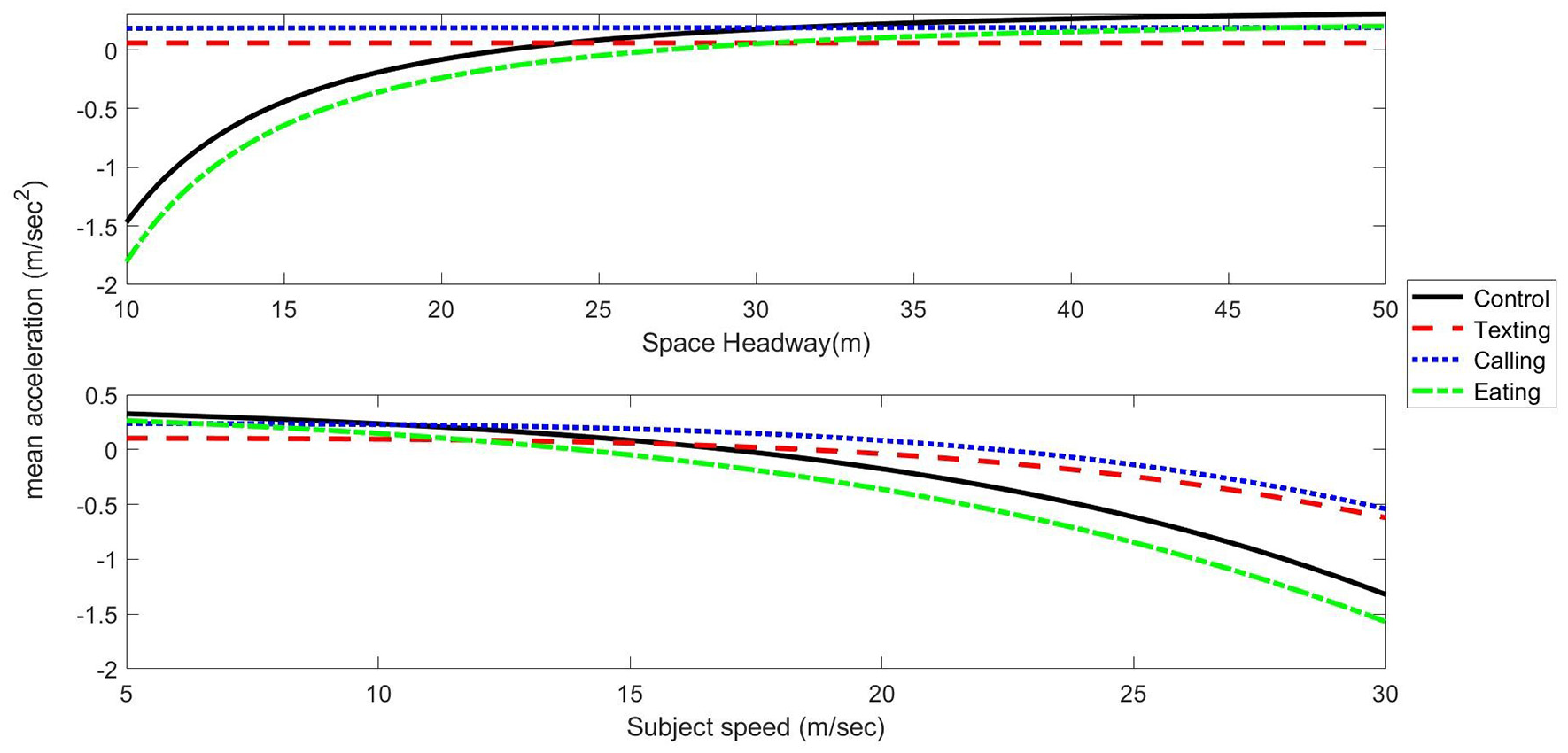
Effects of different variables on mean car-following acceleration in the intelligent driver model (IDM).
Overall, the estimation results of the two models show differences in the car-following behavior among the various conditions. Specifically, driving while texting is significantly different from the other three conditions. In this condition, and to a lesser extent in the talking condition, accelerations are much less sensitive to the relevant variables of subject’s speed, relative speed, and spacing compared with the other conditions. This result is in line with previous studies that showed lower ability to perceive and react to the environment in driving, especially with visual distraction (e.g., 6, 7, 33–35).
Micro-Simulation Implementation
The microscopic traffic simulation model TRANSMODELER was used to evaluate the effect of distracted car following on traffic flow. The GM model is the default car following in TRANSMODELER. The parameter estimates presented above, after additional calibration that will be described below, were used in the simulations. The modified simulation model was applied to a case study of a 6 km arterial corridor in Nesher, Israel, for which TRANSMODELER has been previously calibrated. The corridor includes 17 signalized intersections. The simulation was run for the morning peak period from 7:45 to 9:30 a.m. The trip demand for this corridor was estimated from turning movement counts that were available for all intersections. A total of 12,909 vehicles per hour use this corridor during the morning peak hour. In the simulations, the first 15 min and the last 30 min were used as warm-up and cool-down periods, with 50% of the peak hour demand. The statistics reported in the results are for the vehicles departing in the peak hour from 8:00 to 9:00 a.m.
The car-following models were estimated with data that was collected from a driving simulator. The literature shows that driving simulators are useful to study driving behavior but that drivers’ sensitivity to stimuli from the environment may be lower than in the real world. Therefore, multiplication factors were added to the sensitivity parameters of each model:

where
The values of these two factors were calibrated such that the weighted difference between the average link speeds and flows obtained in the simulation with the previously calibrated TRANSMODELER parameters and the parameters that were estimated for the control condition are minimized:
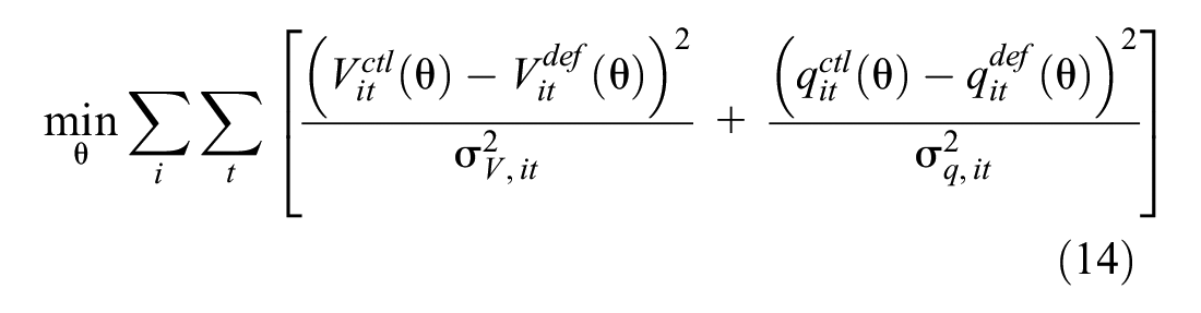
where
The objective above was minimized with
In the traffic simulation experiments, first, all drivers were assumed to be in one of the distraction conditions: either 100% are eating, talking, texting, or not engaged in any secondary activity (control). As will be shown below, traffic flow and safety measures of performance were substantially worse for the texting scenario. Therefore, scenarios with varying percentages of the drivers that are involved in texting (20%, 40%, 60%, 80%) were run next. The remaining drivers were assumed to not be involved in any distracting activity. In each case, five simulation replications were run.
Several measures of performance were calculated from the simulations to indicate traffic flow and safety in each case. The measures used are:
Average speed, which measures the traffic flow level of service. Many studies have also shown its positive association with increases in the likelihood of road crashes and their severity (e.g., 40, 41).
Coefficient of variation (COV) of the speed, which captures speed variability. This has been shown to be positively associated with higher crash rates (e.g., 42, 43). It is calculated as the weighted average of the COVs for all the links in the network:

3. Acceleration noise, which is defined as the standard deviation of the acceleration. It measures the smoothness of traffic flow (e.g., 44–48).
4. Time fraction in acceleration and deceleration, which indicates the variability in acceleration. Higher values of braking time are associated with increased crash risk. It is calculated as the fraction of time that the deceleration is larger than 0.25 m/s2. Similarly, the deceleration time fraction is when the acceleration is larger than 0.25 m/s2. These boundary values represent normal acceleration and deceleration, and so were selected to eliminate low acceleration or deceleration situations (48, 49).
Simulation Results
Table 5 shows the measures of performance values for the scenarios with 100% of drivers undertaking the various distracting activities. The texting and talking on the phone activities reduce the average travel speed compared with the control and cause an increase in the COV of speed. Both these effects are largest for texting. As was seen in the estimation results, with these activities, drivers are less responsive to their environment. For both the average speed and speed COV, the differences among the scenarios are all statistically significant with p-value
Performance Measures and Their Standard Errors by Distracting Activities
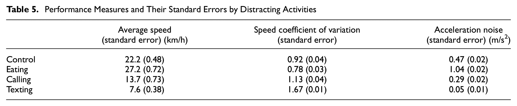
In contrast to these, the acceleration noise is smaller for the texting scenario. This again stems from the lower responsiveness of the drivers to their leader while texting. The acceleration noise is also affected by the level of congestion and the resulting travel speeds: With increased congestion (and lower speeds), vehicles have fewer opportunities to accelerate. The congestion levels differ among the four conditions, and so the results may be misleading. To account for this effect, Figure 5 presents the time fractions in acceleration and deceleration for various ranges of travel speeds. Generally, the fraction of time in both acceleration and deceleration are close to zero in low speeds and increase with speed. With all speed ranges, the acceleration fraction is smallest and the deceleration fraction is largest with texting. Compared with the control case, the differences while texting are statistically significant (p-value < 0.001) for all speed ranges over 20 km/h, for both acceleration and deceleration time fractions. There are no significant differences among the other three conditions. This indicates lower ability of the driver to smoothly control their speed. These results are consistent with the findings of Farah et al. ( 43 ).
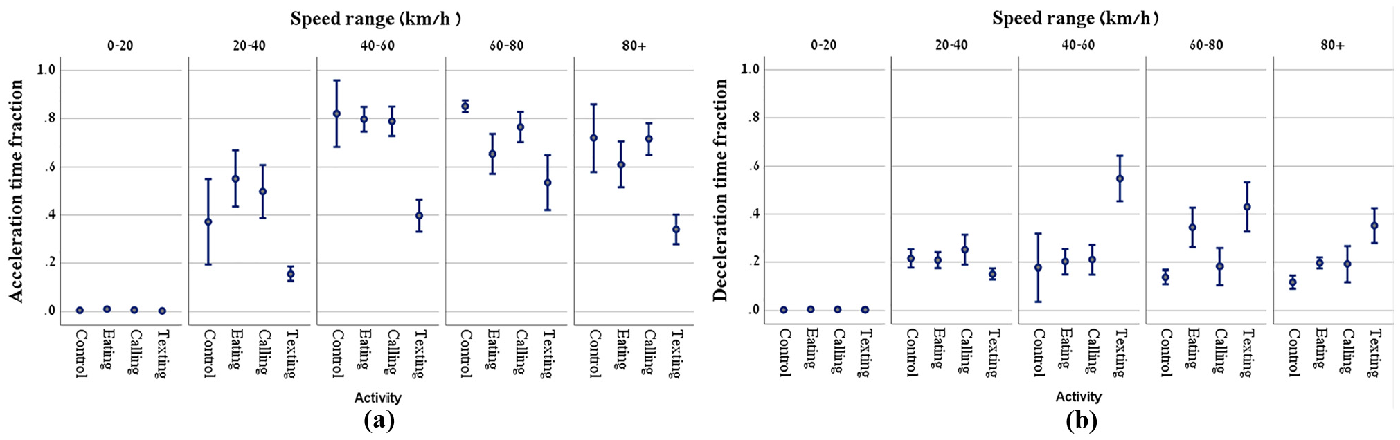
Time fractions in (a) acceleration and (b) deceleration by speed ranges and distraction activity.
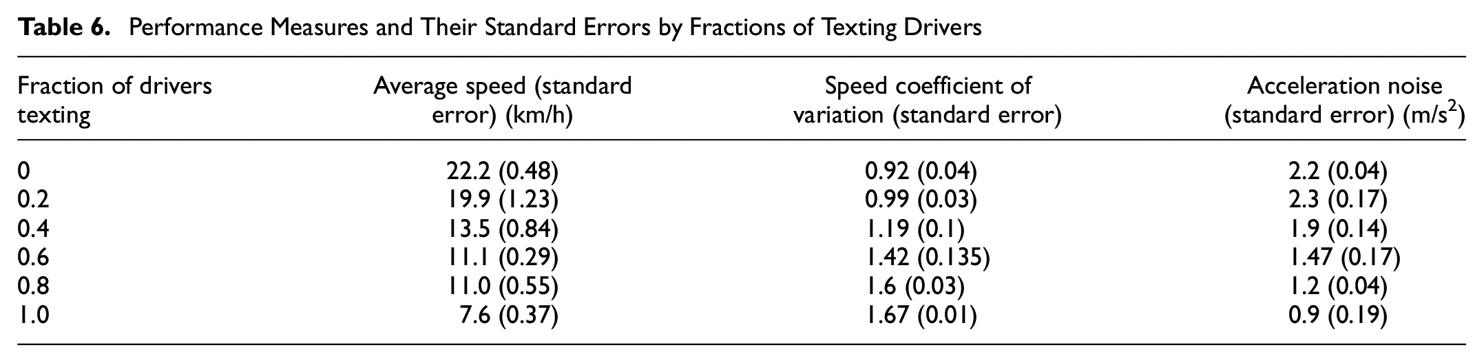
The results above show that texting has the largest effect on driving behavior and the emergent traffic flow characteristics. Therefore, additional experiments were conducted with varying fractions of drivers that are engaged in texting. It is assumed that the other drivers are not distracted (behave according to the control model). The results are presented in Table 6 and Figure 6. The average speed and acceleration noise decrease and the COV of speed increases when the fraction of drivers engaged in texting increases. Compared with the control (no texting drivers), the differences in average speeds are significant (p-value < 0.001) for all fractions of texting drivers that were used in the experiment. The differences in COV of speeds are significant for all fractions of texting drivers (p-value < 0.001), except for 0.2 (p-value = 0.161). These results are expected given the lack of response by drivers to their leaders when texting, therefore, there is greater congestion at intersections and the drivers take longer to complete the simulation.
Performance Measures and Their Standard Errors by Fractions of Texting Drivers
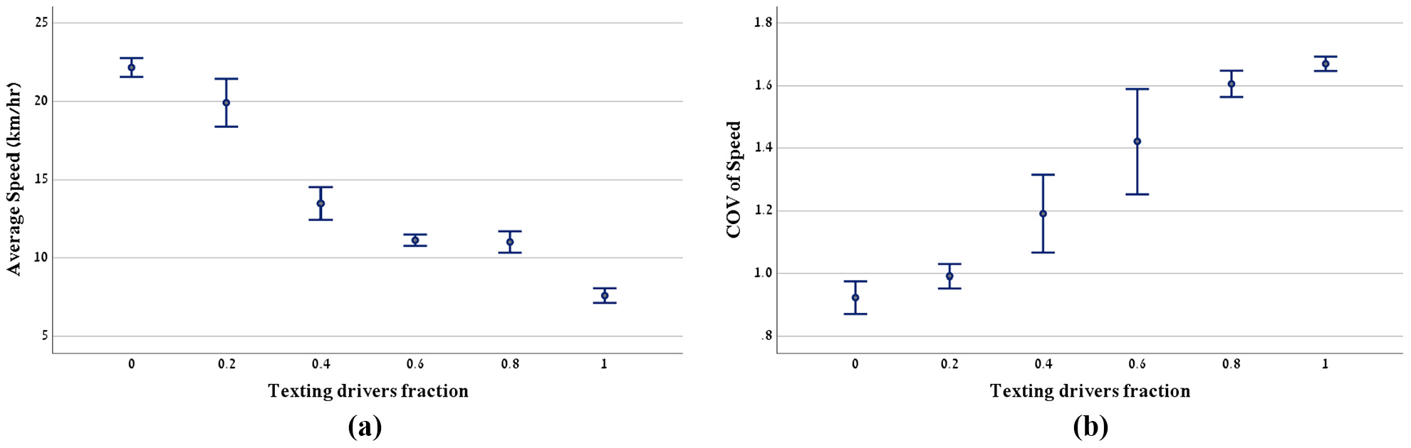
The (a) average of speed and (b) cofficient of speed (COV) by fractions of drivers texting.
The time fractions in acceleration and deceleration as a function of the fraction of drivers that are engaged in texting are shown in Figure 7. The acceleration time fraction decreases and the deceleration time fraction increases with an increase in the fraction of texting drivers. The effects are more pronounced at higher speeds. Compared with the control case (no texting drivers), the differences between the time fractions are statistically significant (p-value < 0.001) for all speed ranges 20–40 km/h or above in acceleration and for all speed ranges 40–60 km/h or above in deceleration. These results again indicate lower response of drivers to their leaders.
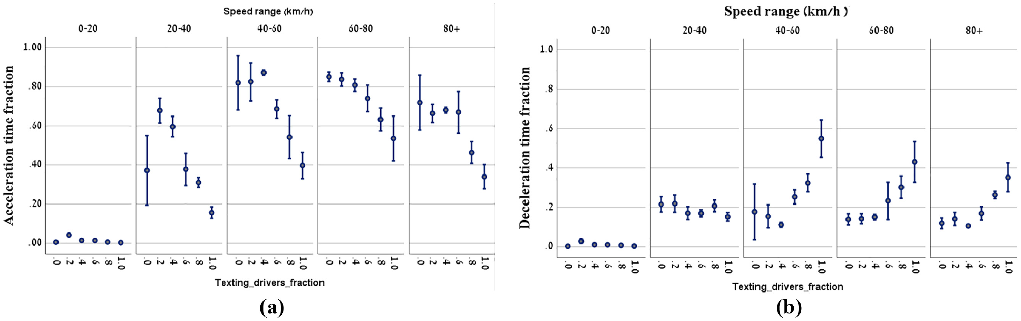
Time fractions in (a) acceleration and (b) deceleration by speed ranges and fractions of drivers texting.
Conclusion
In this study, the GM and IDM car-following models were re-calibrated using data from a simple car-following scenario within a driving simulator to study drivers’ performance while engaging in distracting activities: texting, talking on the phone, or eating, and a control scenario with no distracting activity. Data on the longitudinal and lateral movements of the vehicles were recorded in the experiment.
Estimation results of car-following models for the different distractions show differences in car-following behavior among the various conditions. Specifically, driving while texting is significantly different from the other three conditions. In this condition, both accelerations and decelerations are much less sensitive to the relevant variables of subject’s speed, relative speed, and spacing compared with the other conditions. These results are consistent across the two models. This indicates lower ability to perceive and react to the driving environment, which is in line with previous studies (e.g., 6, 7, 33–35, 50).
The microscopic traffic simulation model TRANSMODELER was used to evaluate the effect of distracted car-following on traffic flow. The average speed, COV of speed, acceleration noise, and acceleration and deceleration time fractions were used as measures of performance indicating traffic flow and safety. The simulation results show deterioration of traffic flow with texting and, to some extent, talking on the phone: average speeds are lower and the COVs of speeds are higher. Further experimentation with varying fractions of texting drivers showed similar trends.
The current study has several limitations, namely, the study was conducted in a virtual simulator environment, where drivers may behave differently compared with real-life driving ( 28 ). Distractions were defined with specific setups. For example, both talking and texting used hand-held devices. Different setups may affect the results. Future study should also aim to analyze naturalistic data to further confirm the results of this study. The model specifications used in the study account for driver heterogeneity, but do not explicitly include reaction times, which may also capture differences among distraction conditions.
Footnotes
Author Contributions
The authors confirm contribution to the paper as follows: study conception and design: S. Zatmeh-Kanj, T. Toledo; data collection: S. Zatmeh-Kanj; analysis and interpretation of results: S. Zatmeh-Kanj, T. Toledo; draft manuscript preparation: S. Zatmeh-Kanj, T. Toledo. All authors reviewed the results and approved the final version of the manuscript.
Declaration of Conflicting Interests
The author(s) declared no potential conflicts of interest with respect to the research, authorship, and/or publication of this article.
Funding
The author(s) disclosed receipt of the following financial support for the research, authorship, and/or publication of this article: This research was supported in part by a grant from GIF, the German-Israeli Foundation for Scientific Research and Development, and by ISF, the Israeli Science Foundation.