Sage Journals: Discover world-class research

Abstract

In this paper, a trajectory control approach using model predictive control is proposed for cooperative (automated) vehicles. This control approach optimizes accelerations of the controlled connected and automated vehicle (CAV) platoon along a corridor with signalized intersections. The objectives of the proposed approach are to maximize the throughput first and optimize comfort, travel delay, and fuel consumption simultaneously after that. The throughput is determined according to the maximal number of CAVs that can pass the intersection during the green phase. Safety is included by penalizing smaller gaps between CAVs in the running cost. The red phase is taken into account as a virtual vehicle at the stop-line during the red time, thus the safe gap penalty with the virtual vehicle causes the first-stopping vehicle to decelerate or even stop facing the red phase. The acceleration and speed are constrained within the upper and lower bounds. The proposed approach is flexible in dealing with platoon merging, splitting, stopping, and queue-discharging characteristics at signalized intersections. Finally, the proposed control approach is verified by simulation under a baseline scenario and four scenarios, which consider signal settings and the anticipation of the red phase. The simulation results demonstrate the benefits of the proposed control approach on fuel savings, compared with the state-of-art approach which used the virtual vehicle term without anticipation. The adjustments of signal parameters in Scenario 3 and Scenario 4 demonstrate the applicability of the control approach under actuated signal control.

Although a considerable amount of work has been done to mitigate urban congestion, traffic delays are still urgent problems on urban roads ( 1 ). In addition, the deceleration and acceleration maneuvers of traditional vehicles in the vicinity of signalized intersections produce high levels of emissions ( 2 ). The current advances in connected and automated vehicle (CAV) technology have the potential to operate vehicles in an efficient, safe, and environmentally friendly way ( 3 ). CAVs can exchange information under vehicle-to-vehicle (V2V) and vehicle-to-infrastructure (V2I) communication, which provides possibilities for anticipation and cooperative driving ( 4 ). Thus, numerous research efforts have been conducted to improve traffic operations by using CAV technologies at signalized intersections ( 5 ).

Current literature on CAV platooning on urban roads can be categorized into four directions, that is, driver assistant systems, cooperative vehicle intersection control algorithms, CAV trajectory optimization, and the integrated optimization of traffic signals and vehicle trajectories.

Driver assistant systems, such as GLOSA (Green Light Optimized Speed Advisory) ( 6 – 8 ) and Eco-Approach and Departure systems ( 9 – 11 ), are able to provide speed advice to drivers at signalized intersections for eco-driving. The purpose of these systems was to operate vehicles in such a way that vehicles arrived at the stop bar in green phases without stopping by calculating the advisory speed based on pre-defined rules. Therefore, the travel time and the fuel consumption were reduced at signalized intersections for the single-subject vehicle. Although further applications of actuated signal plans, market penetration rates, and the extension to multiple intersections were studied ( 6 , 10 , 11 ), the traffic and vehicle dynamics models were usually oversimplified, making the results less convincing. Furthermore, in reality drivers may not comply with the advisory speed and may not control the vehicle speed perfectly as suggested, thus the effects of these systems were required to be validated in field experiments. The empirical validation was only tested in few studies, considering the partial automation ( 9 ) or the adaptive signal control ( 12 ). In addition, these systems were designed only for the individual vehicle benefits, rather than the benefits of the platoon or the traffic flow.

A cooperative vehicle intersection is a “signal-free” intersection which enables the CAVs to communicate with each other and thereby pass the intersection cooperatively without collision ( 13 ). Although these intersection control algorithms had the potential to improve the traffic operations of CAVs at a typical four-arm intersection ( 14 – 17 ) or along a corridor ( 18 ), driver/user acceptance in relation to safety perception and potential conflicts of pedestrians and bicyclists have been neglected, which questions the applicability of this line of research in reality.

With respect to the CAV trajectory optimization by controlling speeds or acceleration rates at fixed-timing intersections, some CAV trajectory control approaches at isolated intersections only applied simple objective functions to optimize energy economy, ride comfort, or both ( 19 , 20 ). These control algorithms used terminal costs to represent the red phase, assuming that the terminal conditions (time and position) were known at an isolated intersection. However, terminal costs are confined to be applicable at isolated intersections, because it is difficult and suboptimal to combine intersections along an arterial using terminal costs. Several instantaneous fuel consumption, emission models, or both ( 21 – 23 ) were adopted in these control approaches to minimize the fuel use, or to validate the reduction of fuel consumption and emission by simulation. More sophisticated systems on corridors with multiple pre-timed intersections were designed for an individual vehicle considering multiple criteria ( 24 – 29 ). The key in the design was supposed to make vehicles stop facing the red phase. There are three ways to achieve this performance: using a virtual vehicle, tracking the target speed, and constraining the position. The first approach applied a virtually preceding vehicle at the stop bar representing the red phase. Together with the safe gap requirement, the followers behind the virtual vehicle were able to stop to keep the safe gap between the virtual vehicle and the followers. The control approach in Asadi and Vahidi ( 24 ) considered the red phase in constraints by introducing a virtual vehicle in front, but the signal information was implemented with no prediction. The other approach aimed to track the piecewise target speed (including desired deceleration rates/speeds) facing the red phase ( 25 – 28 ). To track the pre-defined target speed would produce large decelerations once the vehicle was recognized to miss the green phase, and then accelerate dramatically at the beginning of the green phase. Therefore, more attention should be paid to design the target speed in an optimal way, and relieve computational burden when tracking the piecewise target speed cost term. Another approach was to regard the red phase as a position constraint that the stopping vehicle could not pass ( 29 ). However, the work in Liu et al. ( 29 ) did not track the preceding vehicles in desired gaps. Therefore, elaborate work on tuning cost weights was necessary to make a trade-off between maximizing speeds and minimizing fuel consumption. Otherwise, the vehicles might stop far away from the intersection to save fuel. A parsimonious shooting heuristic algorithm was proposed subject to constraints of vehicle arrivals, vehicle mechanical limits, traffic lights, and car-following safety. The vehicle trajectory was decomposed into a few analytically solvable sections for a simple constructive heuristic. Based on this algorithm, an optimization framework was proposed, optimizing the travel time, a surrogate safety measure, and fuel consumption simultaneously ( 30 , 31 ).

There were also research interests focusing on the integrated optimization of adaptive traffic signals and vehicle trajectories in a unified framework ( 32 – 34 ). The platoons were designed to decelerate but not stop when approaching the intersection during the red phase. However, these control algorithms were designed to optimize simple objective functions of the platoon leader in the vicinity of an isolated intersection for relieving computational load.

From the discussion above, it can be concluded that most current approaches only optimize the trajectories of an individual vehicle using simple objective functions of a few criteria. In addition, it is evident that the existing optimization-based control algorithms under traffic signals mostly focus on design for pre-timing signals, and the current way to represent the red phase using piecewise target speed term may result in computational issues. The previous work in Liu et al. ( 29 ) was designed for an arterial by optimizing a comprehensive objective function, considering throughput, ride comfort, travel delay, and fuel savings. However, the previous control system was open-loop based on feedforward optimal control, and thereby was restricted to a fixed-timing signal plan. One advantage of closed-loop control systems over open-loop systems is that the use of feedback allows the system to be insensitive to both external disturbances and internal variations in system parameters ( 35 ), such as changes in signal settings. Although the control approaches allowed for system feedback in other work ( 19 , 24 , 25 , 28 ), they did not take advantage of it and were thereby confined to pre-timing signals. The reason is that signal information in these approaches is an input when tracking the pre-defined target speed, which excludes signal changes within the system. To include the adaptive signal plan, a closed-loop system is developed to overcome the limitations of open-loop systems. The feedback at each time step in the closed-loop can replan the trajectory under actuated or semi-actuated signal plans. In addition, the previous work in Liu et al. ( 29 ) required elaborate work on tuning cost weights to avoid stopping away from the stop-line. An improvement to address this problem is to transform the red phase position constraint to a penalty term in the running cost, which helps tune the cost weights under the workings of both the safe following and red phase terms.

In this paper, a model predictive control (MPC) framework is proposed for urban corridors under traffic signals to overcome the aforementioned limitations of platoon trajectory control approaches. The proposed MPC framework is efficient on computational time using an iterative Pontryagin maximum principle (iPMP) approach ( 36 ). An optimal platoon trajectory control algorithm is presented by optimizing accelerations of the overall controlled CAV platoon. The control algorithm determines the optimal throughput first, and then optimizes multi-criteria including ride comfort (by minimizing accelerations), average travel delay (by maximizing vehicle speeds), safe space gap, and fuel consumption rates, subject to admissible constraints on acceleration and speed. Safety requirements are incorporated by stimulating the inter-vehicle distances larger than the minimum safe gap as a penalty term in the running cost. The red phases are represented by introducing virtual vehicles at the stop bars during the red phases, thus the first-stopping vehicles can avoid departure in red time using the safe gap penalty with the virtual vehicles. The red phase is implemented with anticipation by updating the cost terms in the running cost at the beginning of the current signal cycle. The proposed control approach is flexible in accounting for platoon dynamics of merging, splitting, stopping, and queue discharging along a corridor with multiple intersections in an oversaturated traffic flow. The proposed trajectory control approach is not restricted to fixed signal timing. It also works under the actuated signal plan by updating the signal parameters in the closed-loop, which reveals the flexibility of the control approach under different signal control approaches. Finally, the performance of the proposed control algorithm is verified by simulation using four scenarios and a baseline scenario, which take the signal settings and the anticipation time of the red phase into account.

The remainder of the paper is organized as follows: the following section introduces the control formulation for longitudinal driving task, followed by the experiment design and analysis of the simulation results. We conclude the study in the final section.

Control Formulation

The longitudinal platoon control problem is formulated in this section, including control problem, control objectives and constraints, system dynamics, controller formulization, running cost specification, derivation of the optimal control input and solution approach.

Control Problem

To demonstrate the workings of the proposed algorithm a 100% CAV environment and pre-timed signal control are considered. It is assumed that signal phasing and timing information is available for the platoon controller under I2V communication, and CAVs can communicate with each other and be controlled via accelerations. The actuator lag and the sensor delay are not considered. Merging behaviors from side streets or adjacent lanes are not taken into account.

The statement of the control problem can be described as a CAV platoon traveling on the corridor with multiple intersections where downstream CAVs are queuing before the stop-lines. The platoon trajectory control system will be activated if the platoon leader reaches the control zone (e.g., 200 m upstream of the stop-line at the upcoming intersection). The control objective is to determine the accelerations of the CAV platoon and CAVs in the queue to fulfill control objectives and constraints. The maximal throughput is pre-determined, and will be detailed in the forthcoming subsection.

Control Objectives

The control design is expected to fulfill (a trade-off between) the following control objectives, including:

To maximize the throughputs during the (remaining) green phases

To maximize the ride comfort (by minimizing accelerations)

To minimize the travel delay (by maximizing vehicle speeds)

To minimize the fuel consumption

To maintain the safe gap with the preceding vehicle

To decelerate or even stop confronting the red phase if unable to pass the intersection

The throughput is optimized first by determining the maximal number of vehicles that are able to pass the intersection during the green phase. The reason for that is to confirm the first-stopping vehicle facing the red phase, and then the red phase term of the sixth objective will be applied to the first-stopping vehicle.

System Dynamics Model

To describe the longitudinal dynamics model, a second-order model is proposed in this subsection. The control input variable u is the acceleration, u_i(t). i (1≤i≤N) denotes the vehicle sequence number on a single lane, and N is the total vehicle number in the controlled platoon. State variables x are considered as the longitudinal position, x_i(t), and the speed, v_i(t), of the controlled vehicle i. The control and state variables can be defined as:

u = {(u_{1}, . . ., u_{i} . . ., u_{N})}^{T}

(1)

x = {(x_{1}, . . ., x_{i} . . ., x_{N})}^{T}

(2)

x_{i} = (\begin{matrix} x_{i} (t) \\ v_{i} (t) \end{matrix})

(3)

The longitudinal dynamics model is described by the following ordinary differential equation:

\frac{d}{d t} x_{i} = \frac{d}{d t} (\begin{matrix} x_{i} (t) \\ v_{i} (t) \end{matrix}) = f (x_{i}, u_{i})

(4)

f (x_{i}, u_{i}) = A x_{i} + B u_{i}

(5)

where

A = [\begin{matrix} 0 & 1 \\ 0 & 0 \end{matrix}]; B = [\begin{matrix} 0 \\ 1 \end{matrix}]

Controller Formulization and Running Cost Specification

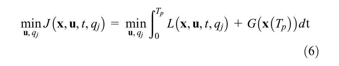
If q_j (veh) denotes the maximal number of vehicles able to pass the jth intersection, then the cost function J of the control system can be formulated as the following:

min_{u, q_{j}} J (x, u, t, q_{j}) = min_{u, q_{j}} \int_{0}^{T_{p}} L (x, u, t, q_{j}) + G (x (T_{p})) d t

(6)

subject to

the system dynamics model of Equation 4

the initial condition: x(0) = x₀

the constraints on state and control variables: x(t) ∈X, u(t) ∈U, t∈ [0, T_p]

where L denotes the running cost and G denotes the terminal cost at the end of the prediction horizon T_p. Although the terminal cost function has an influence on the controller stability and performance, a longer prediction horizon can compensate this impact of G at the cost of computational load ( 37 ). The terminal cost G (=0) and an appropriate prediction horizon are chosen in this work to guarantee the controller performance. Noteworthy is that the maximal throughput q_j can be pre-determined before the final optimal solution. The value of q_j can be optimized beforehand based on the optimal position trajectory x_i(t) when removing the red phase penalty in the control objectives. In other words, the last vehicle that can depart the jth intersection during the green phase is pre-determined as the q_jth vehicle. Here, the first vehicle unable to pass behind the q_jth vehicle is defined as the first-stopping vehicle (i = q_j + 1) at the jth intersection.

In this control design, the running cost of vehicle i, L_i (a constituent of L), is defined as follows (the time t is omitted to simplify equations):

\begin{matrix} L_{i} (x, u, t, q_{j}) = β_{1} {u_{i}}^{2} - β_{2} v_{i} + β_{3} \frac{{(v_{i - 1} - v_{i})}^{2}}{x_{i - 1} - x_{i} - l_{i}} \\ + β_{4} {(x_{i - 1} - x_{i} - v_{i} t_{min} - s_{0} - l_{i})}^{2} \\ + β_{5} f_{eco} (u_{i}, v_{i}) + β_{6} \frac{{(v_{vir}^{j} - v_{q_{j} + 1})}^{2}}{x_{vir}^{j} - x_{q_{j} + 1}} \end{matrix}

(7)

L (x, u, t, q_{j}) = \sum_{i = 1}^{N} L_{i} (x, u, t, q_{j})

(8)

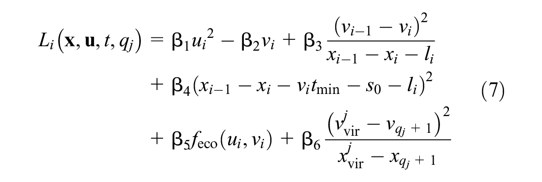
Here, l_i denotes the length of vehicle i, t_min denotes the minimum safe car-following time gap, and s₀ is the minimum space gap at standstill conditions. Turning vehicles to leave intersections can be included in the control approach by setting different values of t_min for different turning movements. To represent the red phase, a virtual standstill vehicle is introduced in the last term of the running cost. $v_{vir}^{j}$ (=0) and $x_{vir}^{j}$ are the speed and the position of the virtual vehicle at the jth intersection, respectively. β₁, β₂, β₃, β₄, β₅, β₆ are cost weights.

The first cost term in the running cost is designed to maximize ride comfort by minimizing accelerations. The second cost term in the running cost is to maximize speeds to minimize travel delay. The third cost term is to track the preceding vehicle and consider the safety as a large penalty if the distance to the predecessor is short. The fourth cost term implies that the gap is stimulated to follow the desired time gap, t_min. The fifth cost term represents the minimization of fuel consumption. The last cost term is designed only for the first-stopping vehicle at the jth intersection (i = q_j + 1) during the red phase. This term renders the stopping vehicles stay in front of the stop-line using the safe gap penalty with the virtual vehicle.

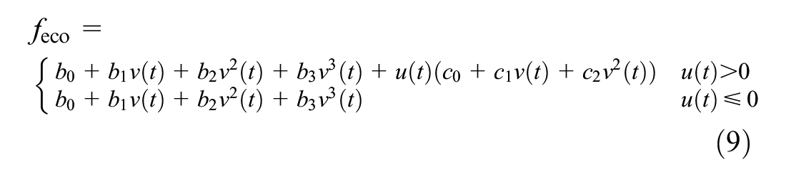
In the fifth term, f_eco is the instantaneous fuel consumption rate (ml/s). Detailed parameter values can be found in Kamal et al. ( 23 ). Although f_eco is optimized to approach zero accelerations and speeds, other criteria in the running cost trade off with the fuel consumption cost to generate optimal trajectories in the vicinity of signalized intersections. For typical vehicles on a flat road, f_eco (ml/s) can be estimated as

f_{eco} = {\begin{matrix} b_{0} + b_{1} v (t) + b_{2} v^{2} (t) + b_{3} v^{3} (t) + u (t) (c_{0} + c_{1} v (t) + c_{2} v^{2} (t)) & u (t) > 0 \\ b_{0} + b_{1} v (t) + b_{2} v^{2} (t) + b_{3} v^{3} (t) & u (t) \leq 0 \end{matrix}

(9)

It should be noted that the running cost in Equation 7 is a piecewise function according to the vehicle sequence in the platoon. The running cost is categorized into three modes for better illustration, that is, the leading mode, the following mode, and the first-stopping mode. Leading mode is designed for the platoon leader, thus the third and fourth (safe following and desired time gap) cost terms vanish owing to no preceding vehicle ahead. Following mode is used for the following vehicles, so the sixth (virtual vehicle) term is removed. First-stopping mode is used for the first-stopping vehicle, which engages in avoiding collision with the virtual vehicle and anticipating signals facing the red phase, so the fourth (desired time gap) term is unnecessary.

This switch of the running cost under three modes can be achieved by updating cost weights β₃ and β₄ (leading mode), β₄ (first-stopping mode), and β₆ (following mode). Assuming the signal cycle starts from the green phase, all cost weights can remain unchanged within the cycle. This is beneficial to apply the proposed control approach under an actuated signal plan because the red and green phase lengths are flexible during a signal cycle. In addition, the red phase refers to the red phase with anticipation, which will be illustrated in the “Solution Approach” subsection.

Derivation of the Optimal Control Input

Hereafter, the control problem is solved based on Pontryagin maximum principle. Without providing too much detail, the Hamiltonian H is defined as follows (t is again omitted):

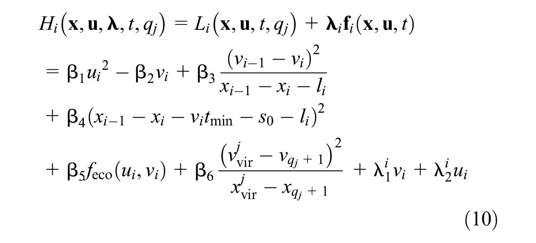
\begin{matrix} H_{i} (x, u, λ, t, q_{j}) = L_{i} (x, u, t, q_{j}) + λ_{i} f_{i} (x, u, t) \\ = β_{1} {u_{i}}^{2} - β_{2} v_{i} + β_{3} \frac{{(v_{i - 1} - v_{i})}^{2}}{x_{i - 1} - x_{i} - l_{i}} \\ + β_{4} {(x_{i - 1} - x_{i} - v_{i} t_{min} - s_{0} - l_{i})}^{2} \\ + β_{5} f_{eco} (u_{i}, v_{i}) + β_{6} \frac{{(v_{vir}^{j} - v_{q_{j} + 1})}^{2}}{x_{vir}^{j} - x_{q_{j} + 1}} + λ_{1}^{i} v_{i} + λ_{2}^{i} u_{i} \end{matrix}

(10)

where $λ$ denotes the co-state of the system:

λ_{i} (t) = (\begin{matrix} λ_{1}^{i} (t) \\ λ_{2}^{i} (t) \end{matrix})

(11)

Thus, the optimal control law can be obtained according to the necessary condition for the optimal control law using Hamiltonian. Therefore, the optimal control law can be described as:

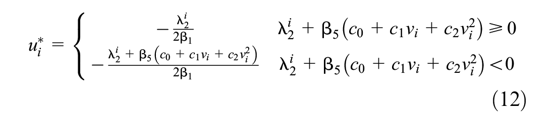
u_{i}^{*} = {\begin{matrix} - \frac{λ_{2}^{i}}{2 β_{1}} & λ_{2}^{i} + β_{5} (c_{0} + c_{1} v_{i} + c_{2} v_{i}^{2}) \geq 0 \\ - \frac{λ_{2}^{i} + β_{5} (c_{0} + c_{1} v_{i} + c_{2} v_{i}^{2})}{2 β_{1}} & λ_{2}^{i} + β_{5} (c_{0} + c_{1} v_{i} + c_{2} v_{i}^{2}) < 0 \end{matrix}

(12)

To simplify the piecewise feature of the instantaneous fuel consumption model f_eco, the Heaviside function h is introduced:

h (n) = {\begin{matrix} 1 & n > 0 \\ 0 & n \leq 0 \end{matrix}

(13)

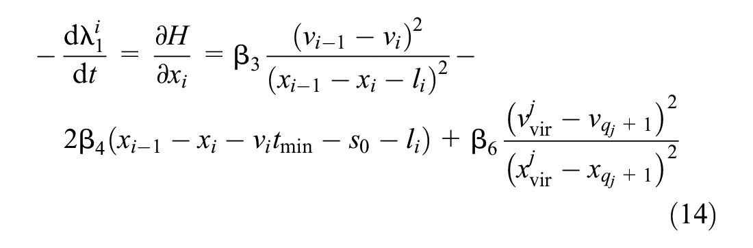
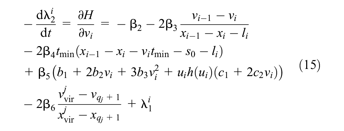
In Equation 13, the Heaviside function value is zero for negative and zero arguments (n≤0), and holds for one under positive arguments (n>0). The co-state dynamics are thereby derived as:

- \frac{d λ_{1}^{i}}{d t} = \frac{\partial H}{\partial x_{i}} = β_{3} \frac{{(v_{i - 1} - v_{i})}^{2}}{{(x_{i - 1} - x_{i} - l_{i})}^{2}} - 2 β_{4} (x_{i - 1} - x_{i} - v_{i} t_{min} - s_{0} - l_{i}) + β_{6} \frac{{(v_{vir}^{j} - v_{q_{j} + 1})}^{2}}{{(x_{vir}^{j} - x_{q_{j} + 1})}^{2}}

(14)

\begin{matrix} - \frac{d λ_{2}^{i}}{d t} = \frac{\partial H}{\partial v_{i}} = - β_{2} - 2 β_{3} \frac{v_{i - 1} - v_{i}}{x_{i - 1} - x_{i} - l_{i}} \\ - 2 β_{4} t_{min} (x_{i - 1} - x_{i} - v_{i} t_{min} - s_{0} - l_{i}) \\ + β_{5} (b_{1} + 2 b_{2} v_{i} + 3 b_{3} v_{i}^{2} + u_{i} h (u_{i}) (c_{1} + 2 c_{2} v_{i})) \\ - 2 β_{6} \frac{v_{vir}^{j} - v_{q_{j} + 1}}{x_{vir}^{j} - x_{q_{j} + 1}} + λ_{1}^{i} \end{matrix}

(15)

Controller Constraints

The control problem should respect some constraints on control and state variables. Admissible acceleration is restricted between the maximum acceleration, a_max, and the minimum acceleration, a_min. Speed should be lower than the limit speed, v_max, but nonnegative.

a_{min} \leq u_{i} (t) \leq a_{max}

(16)

0 \leq v_{i} (t) \leq v_{max}

(17)

Solution Approach

An iPMP approach is applied to solve this control problem, referring to Hoogendoorn et al. ( 36 ) and Wang et al. ( 38 ) for details. The continuous-time control problem is discretized in time within the prediction horizon in relation to the control and co-state variables. The iPMP approach solves the state and co-state dynamics forward and backward in time, respectively, and then updates the co-state dynamic with a weight factor. The updated co-state will be imported to the next iteration as an input. The optimization converges if the error between the state and co-state dynamics is smaller than the pre-defined threshold, then the iteration stops. The illustration of the solution approach is depicted in Figure 1.

Figure 1.

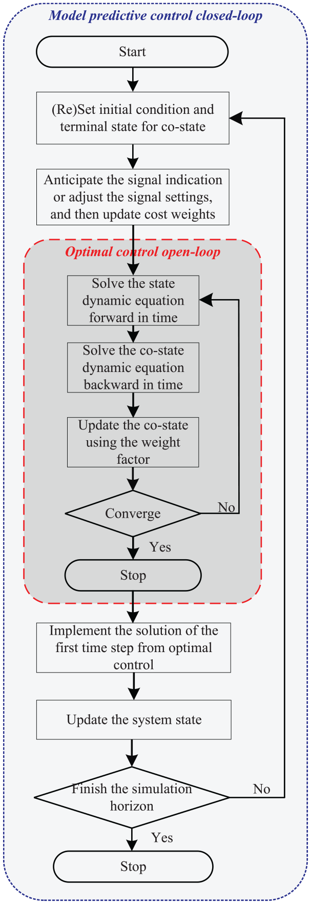
Illustration of the solution approach.

The MPC framework is applied, which solves the control problem in a shorter horizon than the optimal control framework in our previous work ( 29 ). This shorter horizon of the MPC framework results in an efficient computational time. The MPC framework only selects the first time step of the optimal solution in the iPMP algorithm. The constraints on control and state variables are implemented on restricting control variables based on system dynamics.

Platoon dynamics of merging, splitting, stopping, and queue discharging along a corridor are achieved by switching three modes of the running cost (updating the values of cost weights), which is included within the MPC closed-loop at every time step. In the presence of signal anticipation, the red phase can be anticipated by implementing the virtual vehicle term as early as possible, that is, at the beginning of the current signal cycle under the pre-timing signals, or at the moment when the platoon controller receives the updated signal plan under actuated signals. The MPC framework allows for system feedback, that is, signal changes, thus actuated signal settings can also be incorporated in the MPC closed-loop. In addition to signal anticipation, the signal settings (the green and red time) can also be updated in the MPC closed-loop by switching the cost weights in response to the actuated signals. Therefore, this approach can also be applied under the actuated signal control approach.

Simulation Results and Analysis

This section verifies the platoon performances of this control algorithm under four scenarios, considering the signal settings and the anticipation time of the red phase. A baseline scenario is also presented for comparison.

Experiment Design

To test the behavior of the platoons resulting from the proposed control approach, trajectories on a corridor with two signalized intersections are simulated, taking into account the signal settings, the lane length between two adjacent intersections, the speed limit, and the numbers of vehicles in the controlled platoon and in the queue. Four scenarios and a baseline scenario are designed to verify the characteristics of platoon splitting, merging, decelerating, accelerating, stopping, and queue discharging. The control effects on the fuel savings are revealed by comparing the total fuel consumptions of all controlled vehicles within the simulation horizon. Hereafter, the intersection in the upstream direction on the arterial is referred as the upstream intersection, and the intersection in the downstream direction is considered as the downstream intersection.

Two pre-timed signal settings are designed to test the workings of the red phase term, that is, the opposite and overlapped signal settings, as shown in Figure 2. The length of the effective green phase is 30 s in both settings, whereas the effective red phase is 30 s and 20 s in opposite and overlapped signal settings, respectively. Therefore, the simulation horizons are 90 s and 80 s separately in different signal settings. The prediction horizon is selected to be 10 s, because the influence of the zero terminal cost is negligible with respect to 5 s and larger prediction horizon ( 37 ).

Figure 2.

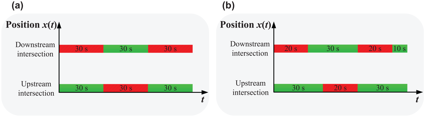
Design of signal settings; (a) opposite signal setting, (b) overlapped signal setting.

In reality, the communication ranges of I2V and V2V are about 200 m, thus the control zone starts from 200 m away from the stop bar in the upstream direction at the upstream intersection. The longitudinal position of the stop-line at the upstream intersection is defined as 0. The lane section length between two adjacent intersections is designed as 800 m, thus the longitudinal position of the stop-line at the downstream intersection is 800.

To test the performances taking signal settings and the anticipation time of the red phase into account, four scenarios and a baseline scenario are designed. These scenarios are appropriate to verify the feasibility of the platoon trajectory control approach in relation to the applications on an arterial with intersections. The characteristics of platoon splitting, merging, decelerating, accelerating, stopping, and queue discharging in all the scenarios provide insights into the effectiveness of the control approach. The benefits on fuel savings are explored in all scenarios. Similar settings (e.g., the number of controlled vehicles, vehicle queues, the number of multiple intersections, and the signal timing plans) can be implemented easily in the same way. The cost weights are tuned in Scenario 1 and then are applied in other scenarios. The parameter values in the simulation are detailed in Table 1. The choices for the parameter values mostly come from previous work ( 29 ). In our experiment settings, the time step is 1 s, which means delays under 1 s have no effect on the optimal trajectories.

Table 1.

Parameter and Coefficient Values in the Experiment

Notation	Parameter/coefficient	Value	Unit
na	time step	1	s
na	prediction horizon	10	s
na	the effective green phase	30	s
na	the effective red phase	20, 30	s
na	initial speed	0, 15	m/s
na	initial space gap in the nonstatic platoon	35	m
na	initial space gap in vehicle queues	5	m
na	the range of the control zone at the upstream intersection	200	m
na	the number of total controlled vehicles	25	veh
na	vehicle queues at the upstream intersection	3	veh
na	the number of vehicles on the lane section between two intersections	8	veh
Y_j	the position of the stop-lines at intersections	0, 800	m
l_i	length of every controlled vehicle	3	m
t _min	minimum safe car-following time gap	2	s
s₀	minimum space gap at standstill conditions	2	m
v _max	limit speed on the urban corridor	20	m/s
a _max	allowable maximum acceleration	2	m/s²
a _min	allowable minimum acceleration	−5	m/s²
β₁	cost weight	1	na
β₂	cost weight	1	na
β₃	cost weight	1	na
β₄	cost weight	1	na
β₅	cost weight	0, 5	na
β₆	cost weight	5	na

Note: na = not applicable.

The baseline scenario is presented under the opposite signal setting without anticipating the red phase. The anticipation of the red phase under pre-timed signal control is removed, thus the virtual vehicle term is added just at the beginning of the red phase. The objective of this baseline scenario is to obtain insights of the validity of the red phase (virtual vehicle) term, which is similar to the application in previous work ( 24 ).

In the forthcoming four scenarios, the anticipation time of the red phase is implemented at the beginning of the current signal cycle. Anticipating the red indication before the start of the red phase is supposed to outperform the baseline scenario where no anticipation exits (e.g., saving more fuel). Scenario 1 is simulated under opposite and pre-timed signal plan with anticipating the red phase. The comparison between the baseline scenario (no anticipation) and Scenario 1 (anticipation from the beginning of the current signal cycle) can explore the benefits of anticipating the red phase in the proposed control approach. Scenario 2 is designed under overlapped and pre-timed signal settings, which can prove the workings of the adjustment in signal settings under pre-timed signal control. In Scenario 3, the actuated signal is included in the MPC closed-loop. The length of green phases increases 5 s whereas the red windows decrease 5 s adaptively based on the overlapped signal settings. Scenario 4 updates the signal plan based on the initial overlapped signal setting according to the oversaturated traffic flow. The lengths of the red (and green) phases in sequence are 15 s and 18 s (17 s and 20 s) at the downstream intersection, and the counterparts are 18 s (27 s and 25 s) at the upstream intersection. The last two scenarios aim to investigate the workings of the proposed control approach under the actuated signal plan. It is assumed that the platoon controller receives the actuated signal plan after the first prediction horizon, that is, 10 s after the beginning of the signal cycle.

Platoon Performance

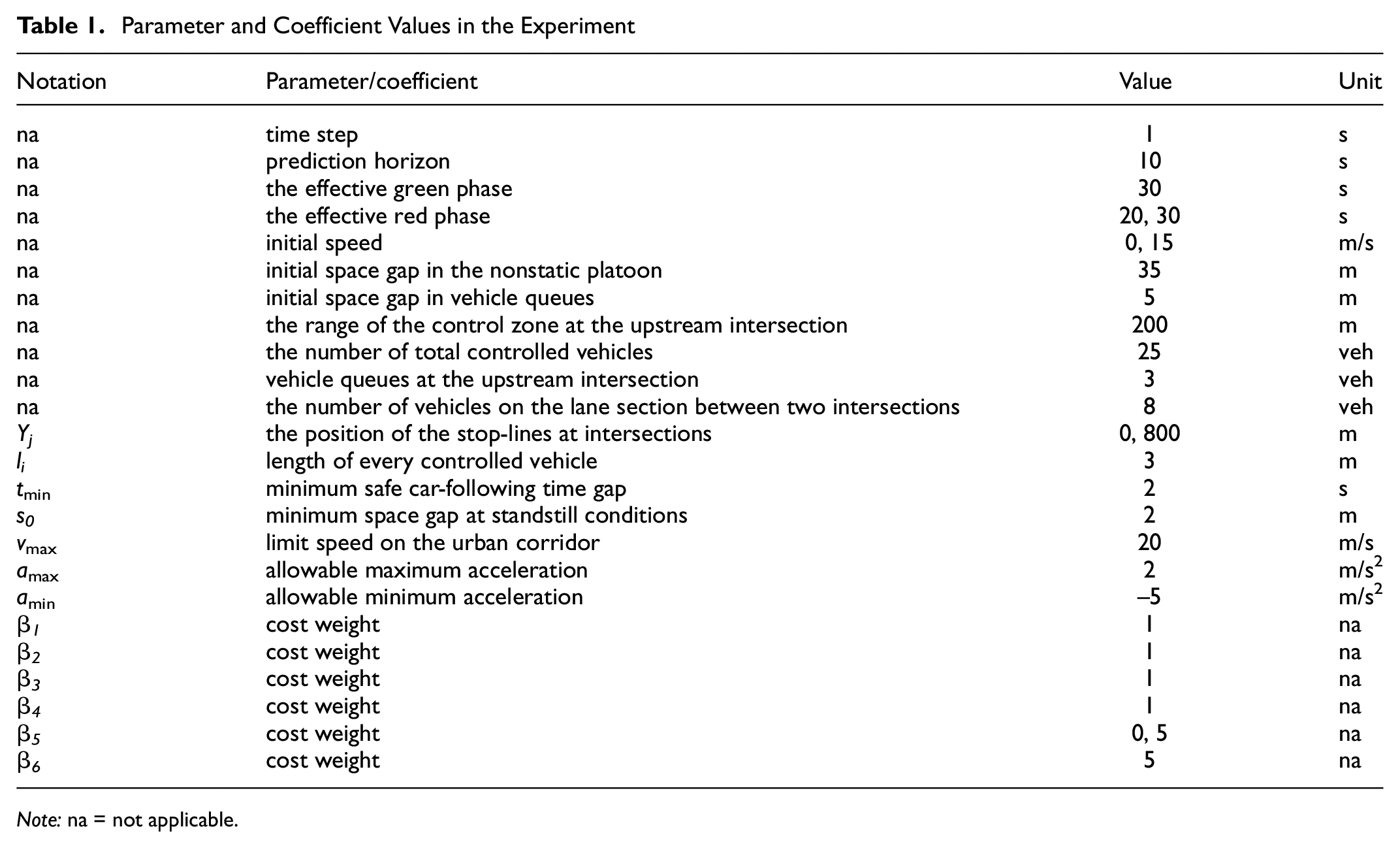
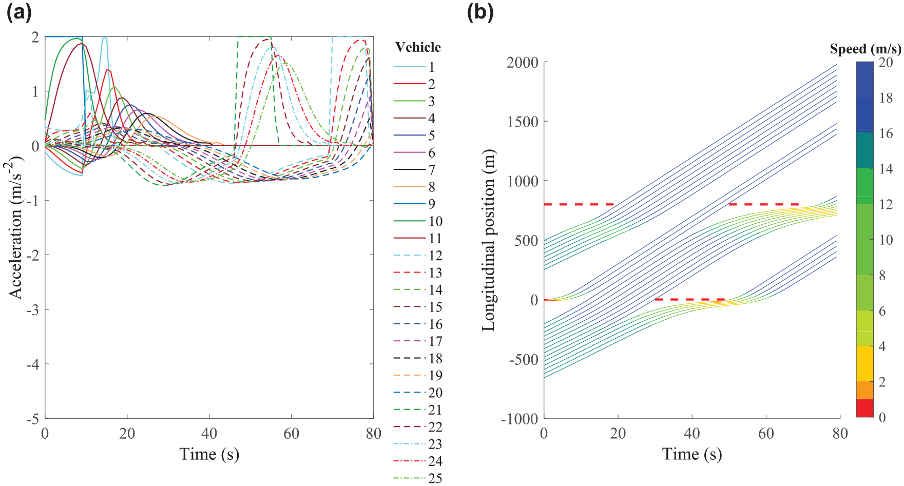
The aforementioned scenarios are simulated to evaluate control effects based on trajectory analysis, as depicted in Figures 3 –7. It is obvious that the safe gap and the red phase penalty work, and the controller constraints are satisfied. The vehicle numbers in the legend represent the vehicle sequence of the platoon on a single lane. The horizontal red dashed lines in these figures show the red signal indication at intersections. The longitudinal positions of the stop-line at the upstream and downstream intersections are 0 and 800, respectively. The initial conditions at the beginning of the simulation are as follows: the first eight vehicles are set with initial speed (15 m/s) on the lane section between two adjacent intersections, after that three vehicles stop (0 m/s) at the upstream intersection, and the last 14 vehicles are traveling (15 m/s) from 200 m upstream direction of the upstream intersection (–200 m).

Figure 3.

Optimal trajectories of baseline scenario: (a) acceleration and (b) longitudinal position.

Figure 4.

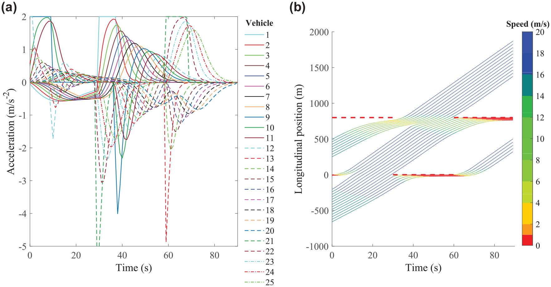
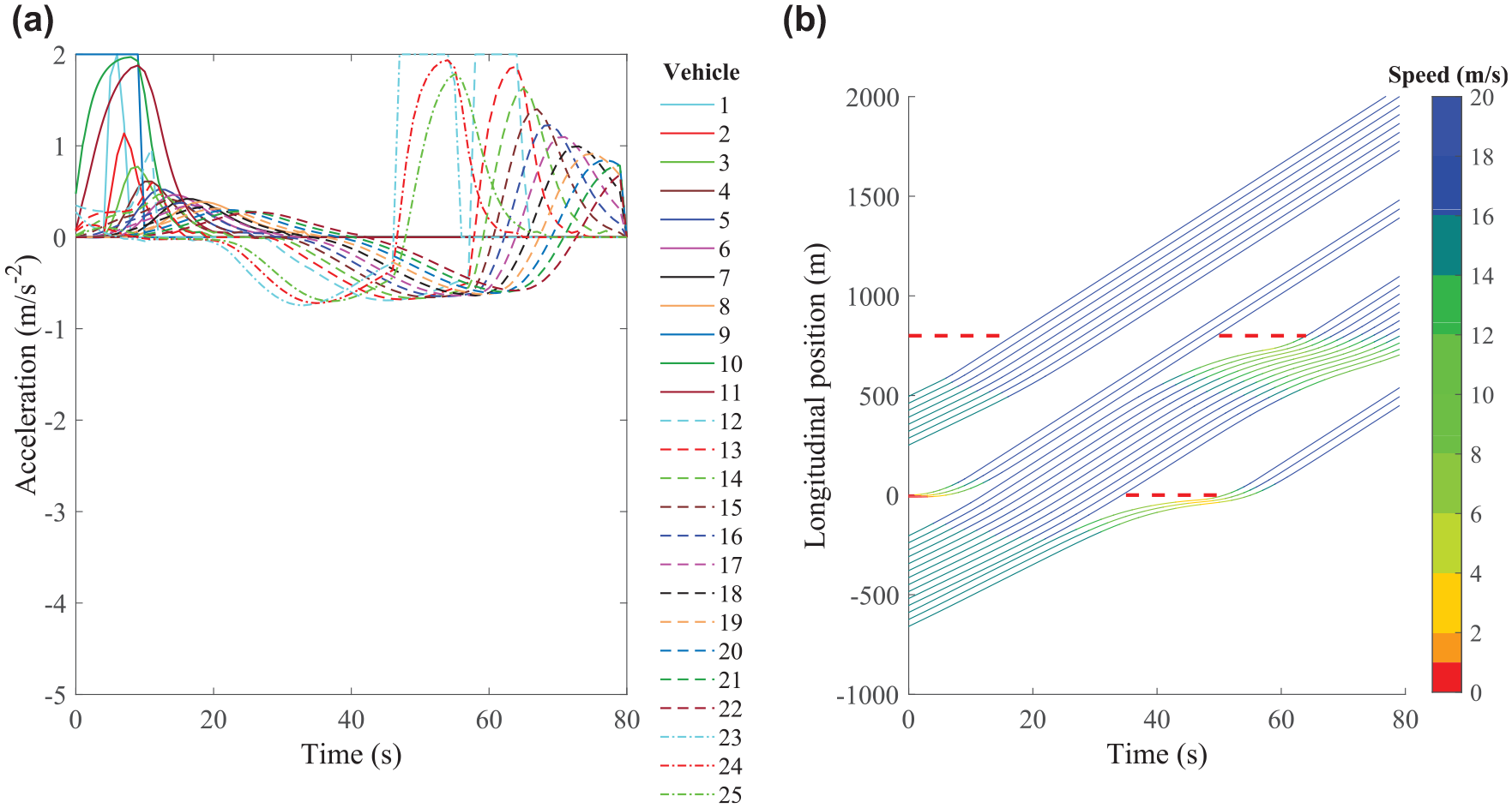
Optimal trajectories of Scenario 1: (a) acceleration and (b) longitudinal position.

Figure 5.

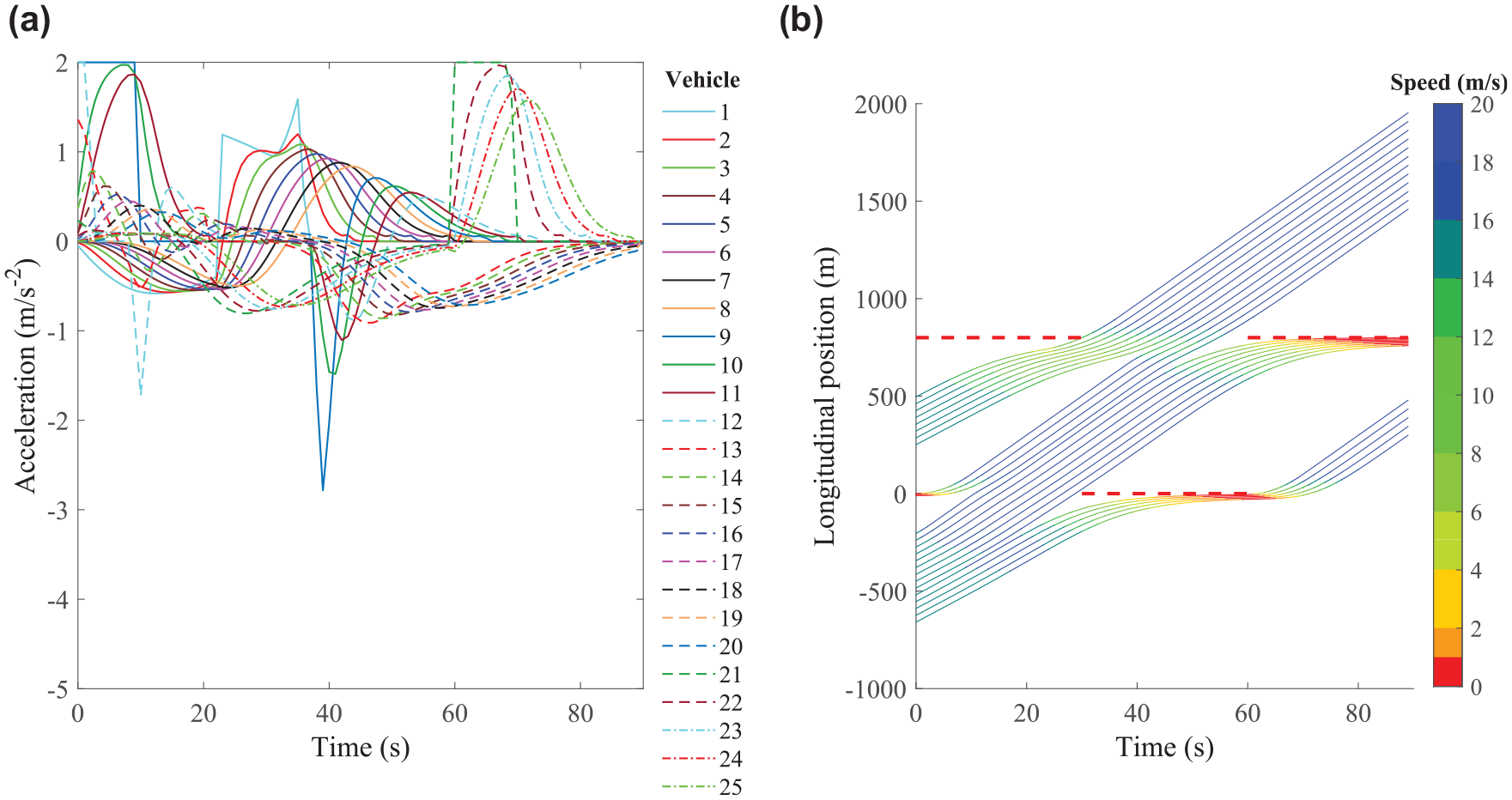
Optimal trajectories of Scenario 2: (a) acceleration and (b) longitudinal position.

Figure 6.

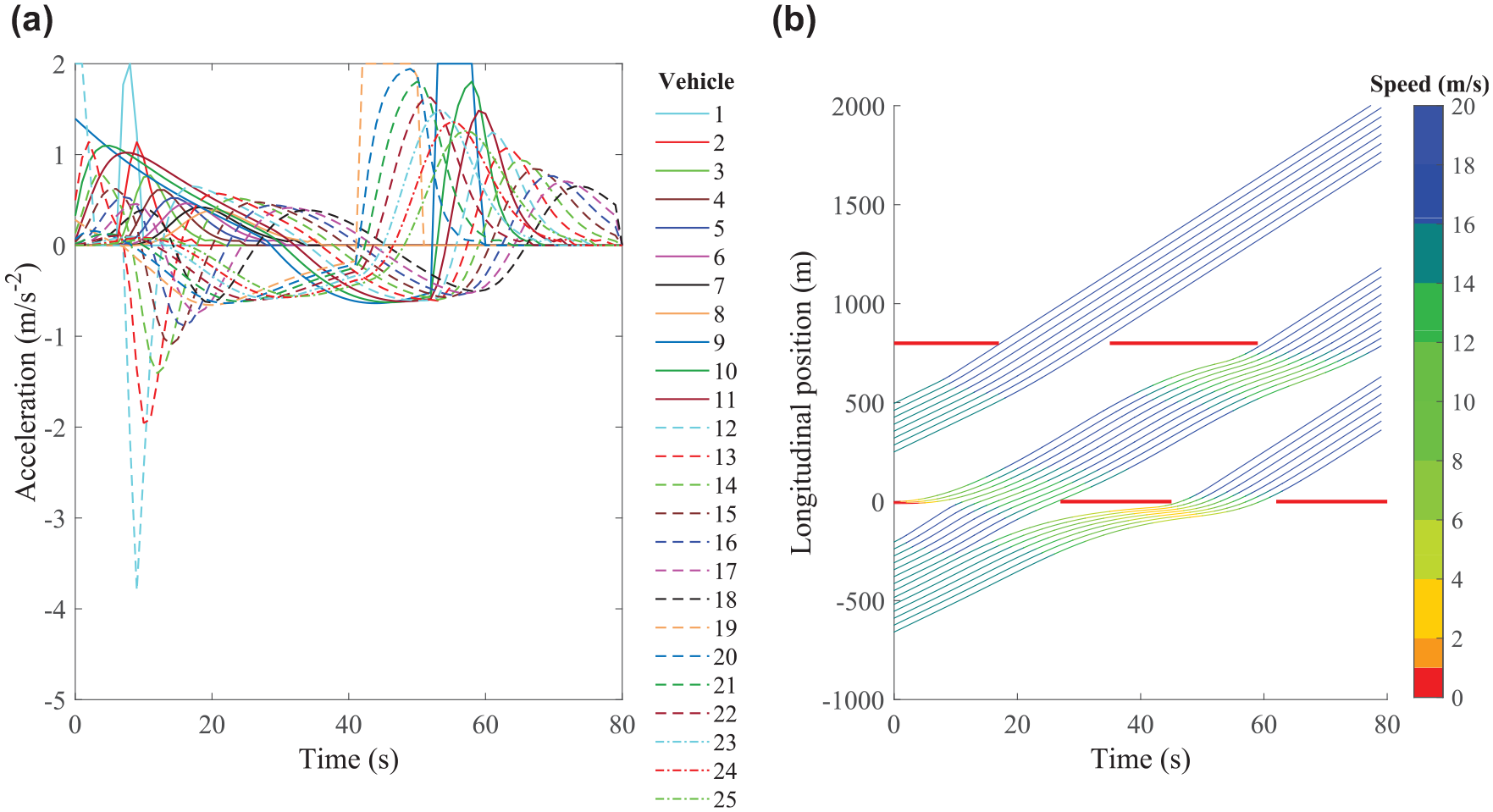
Optimal trajectories of Scenario 3: (a) acceleration and (b) longitudinal position.

Figure 7.

Optimal trajectories of Scenario 4: (a) acceleration and (b) longitudinal position.

The maximal throughputs are determined first when removing the red phase penalty, as discussed in the previous section. To be noted, the iPMP approach is more efficient on computational time, compared with the solver used in Liu et al. ( 29 ) based on the optimal control framework, in spite of similar experiments. The remainder of this section analyzes the platoon performances and spacing gap in each scenario. The advantages of the proposed control approach are discussed in comparison with the baseline scenario.

Tuning Cost Weights

First, the cost weights are tuned to gain insights of optimal trajectories based on Scenario 1. Considering β₁ = 1 as a baseline, the cost weight of speed, β₂, the cost weight of safe gap term, β₃, and the cost weight of the desired gap, β₄, keep the same order with the cost weight of acceleration β₁, thus β₂ = β₃ = β₄ = β₁ = 1. Bigger values of the fuel consumption cost weight, β₅, will result in lower accelerations and speeds, so the maximal throughput cannot be obtained via this overweighed β₅. The biggest value of β₅ (=5) is selected to avoid unnecessary deceleration. Smaller values of virtual vehicle cost weight β₆ are unable to act as the red phase, whereas vehicles will decelerate and stop near the initial position, that is, the known position at the start of the simulation time, if β₆ is too large. The appropriate value of the red phase cost weight, β₆ (=5), is chosen to optimize the vehicles stopping just in front of the stop-line. These values of all cost weights are selected in Scenario 1 and then applied in all scenarios.

Analysis of Baseline Scenario

The baseline scenario represents the situation that no anticipation of the red phase is provided under the opposite signal setting using virtual vehicle term, as shown in Figure 3. The total fuel consumptions of all vehicles within the simulation horizon are 1888.3 ml (0.0606 ml/m) in this baseline scenario. The vehicles in the queue at the upstream intersection (vehicle 9–11) start from 0 speed, whereas other vehicles begin with the initial speed of 15 m/s. The first 12 vehicles are able to pass the downstream intersection, and vehicles 9–20 leave the upstream intersection. These vehicles depart the intersections with accelerating to the limit speed v_max, so the maximal throughput can be guaranteed.

Although the red phase is not anticipated, the vehicles are able to stop in front of the stop-line but with drastic decelerations at the beginning of the red phase (i.e., for vehicle 21 at the upstream intersection at 30 s and for vehicle 13 at the downstream intersection at 60 s). Without the prevision of red phases, the passing vehicles (e.g., vehicles 1–8) are optimized to decelerate during the red phase and then accelerate suddenly at the beginning of the green phase, which causes more fuel consumption. In addition, the stops during the red phase cannot be avoided if the vehicles have to catch the next green phase. To be noted, vehicle 9 decelerates during 38 s to 43 s to keep the safe gap when merging with the preceding platoon. The same holds for vehicle 12 during 10–13 s.

Analysis of Scenario 1

Scenario 1 is simulated under the opposite signal setting but with anticipating the red phase at the beginning of the current signal cycle. The total fuel consumption of all vehicles is 1854.9 ml (0.0579 ml/m) in Scenario 1, which is smaller than the counterpart in the baseline scenario. As shown in Figure 4, the trajectories in Scenario 1 are similar to the baseline scenario, but the fluctuations of accelerations and decelerations are much smoother, especially for the first-stopping vehicles (vehicles 13 and 21). The decelerations of vehicles 9 and 12 remain the same to keep the safe gap with the preceding vehicles while merging (during 38–43 s and during 10–13 s separately). Owing to the anticipation of the red phase, the first-stopping vehicles (vehicles 13 and 21) react more predictively to the red phase and approach the stop-line more slowly in comparison with the baseline scenario, as can be seen in the longitudinal position subfigures Figures 3b and 4b.

The differences in trajectory performances between the baseline scenario and Scenario 1 prove the benefits of anticipating the red phase in the proposed control approach. The sharp decelerations and stops facing the red phase are avoidable, and more fuel savings are verified in Scenario 1.

Analysis of Scenario 2

In Scenario 2, the overlapped signal setting is presented, as depicted in Figure 5. The total fuel consumption of all vehicles is 1736.2 ml (0.0550 ml/m) in Scenario 2. Although the trajectory performances in Scenario 2 keep the same features as in Scenario 1 apart from the signal setting, Scenario 2 validates the flexible characteristic of the control approach in relation to changes in signal settings under pre-timed signal plan.

Analysis of Scenario 3

Scenario 3 explores the potential to implement the proposed approach under the actuated signal plan. The initial signal plan is the same as the overlapped signal settings. However, the signal plan is updated in the MPC closed-loop after the first prediction horizon (10 s) in the signal cycle. The lengths of green phases change with an increase of 5 s, and the lengths of red phases vary with a decrease of 5 s. The total fuel consumption of all vehicles is 1879.2 ml (0.0550 ml/m) in Scenario 3. The optimal trajectories depicted in Figure 6 prove the feasibility of the control approach in relation to application in actuated or adaptive signal plans.

Analysis of Scenario 4

Scenario 4 provides more insights for the proposed control approach being applied with the actuated signal approach under the oversaturated traffic flow. The initial signal plan is the overlapped signal settings, and then signal parameters are adjusted to accommodate changes in the traffic flow, that is, red time of 15 s, green time of 17 s, red time of 18 s, and green time of 20 s in sequence at the downstream intersection; green time of 27 s, red time of 18 s, and green time of 25 s in sequence at the upstream intersection. The total fuel consumption of all vehicles is 1885.1 ml (0.0592 ml/m) in Scenario 4. The optimal trajectories in Figure 7 further validate the workings under actuated signals.

Analysis of Spacing Gap

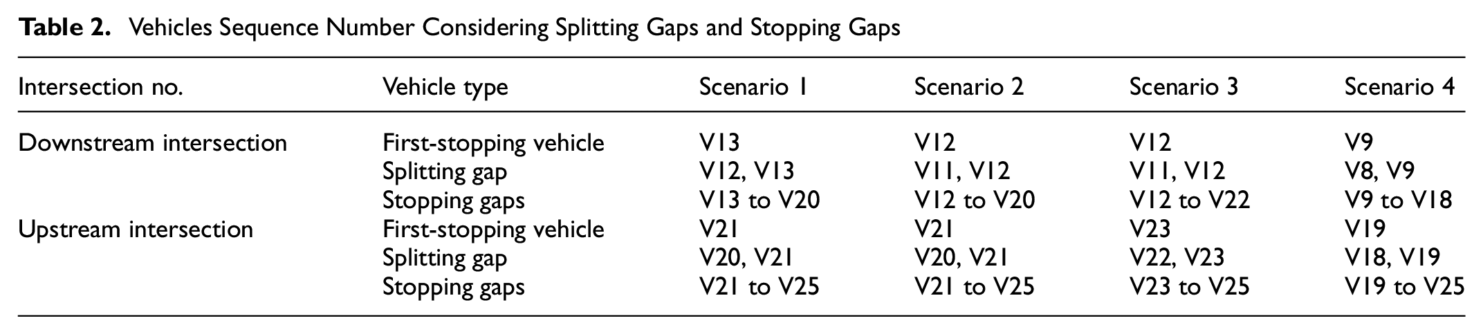
The spacing gaps of all controlled vehicles can be categorized into four groups, that is, the splitting gaps, the stopping gaps, the following gaps, and the merging/catching gaps. The splitting gaps aim to reflect the increases in gaps resulted from the red indication, that is, the gaps between the first-stopping vehicles and the immediately preceding vehicles. For other stopping vehicles behind the first-stopping vehicles, the stopping gaps can describe the gaps between two adjacent stopping vehicles. Table 2 details the vehicle sequence number (represented by V) in relation to the first-stopping vehicles, the splitting gaps, and the stopping gaps under four scenarios at two intersections. The following gaps account for gaps between vehicles that can pass the downstream intersection during the first green phase. The merging or catching gaps are proposed to capture declines in spacing owing to the signal settings and the initial position settings, namely, the gaps between vehicles 8 and 9 and between vehicles 11 and 12. The differences between the merging gaps and the catching gaps are whether the gaps drop into the following gaps within the horizon. It is noted that the merging/catching gap and the splitting gap may occur on a certain vehicle sequentially under different signal phases, for example, in Scenario 2, Scenario 3, and Scenario 4.

Table 2.

Vehicles Sequence Number Considering Splitting Gaps and Stopping Gaps

Intersection no.	Vehicle type	Scenario 1	Scenario 2	Scenario 3	Scenario 4
Downstream intersection	First-stopping vehicle	V13	V12	V12	V9
	Splitting gap	V12, V13	V11, V12	V11, V12	V8, V9
	Stopping gaps	V13 to V20	V12 to V20	V12 to V22	V9 to V18
Upstream intersection	First-stopping vehicle	V21	V21	V23	V19
	Splitting gap	V20, V21	V20, V21	V22, V23	V18, V19
	Stopping gaps	V21 to V25	V21 to V25	V23 to V25	V19 to V25

To explore the performance of spacing, the gaps between two adjacent vehicles under four scenarios are illustrated in Figure 8. The vertical ordinate of the spacing subfigures is presented compactly by way of logarithmic scale. The four spacing gap categories are depicted in different colors and line types. It can be concluded that the spacing gaps are in accordance with the system design, because the space gaps satisfy the safe requirement over the simulation horizon in all scenarios, and the spacing gaps fluctuate with changes in splitting and merging performances and signal changes.

Figure 8.

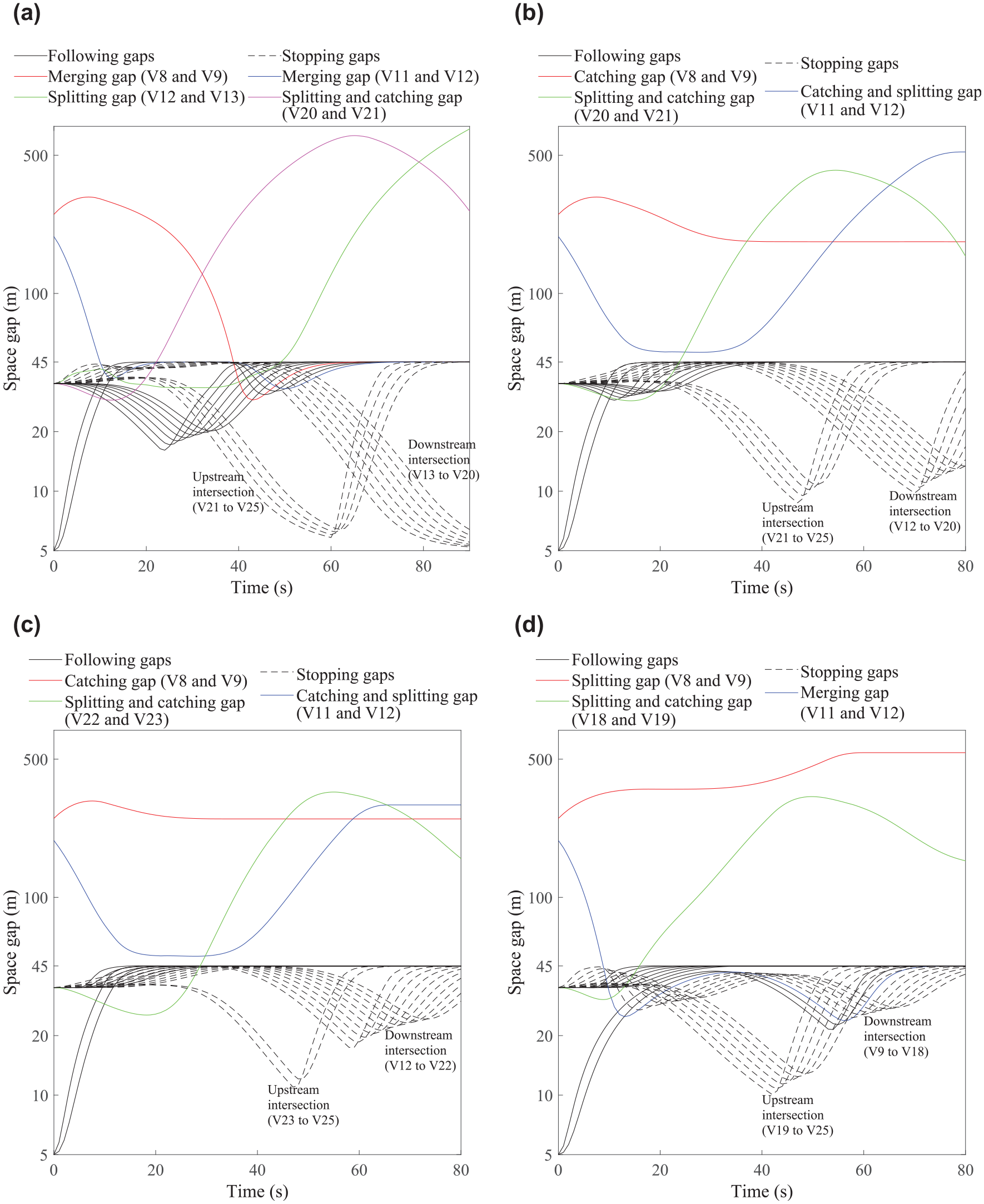
Spacing gap under four scenarios: (a) Scenario 1, (b) Scenario 2, (c) Scenario 3, and (d) Scenario 4.

There are general characters in all scenarios. The initial space gaps are 5 m for queuing vehicles at the standstill condition, and 35 m for the nonstatic vehicles. The maximal following gap is 45 m, which is calculated using v_maxt_min+s₀+l_i. Taking into account the speed constraint which limits the controlled speeds being equal to or lower than the maximal speed, the following and stopping gaps cannot exceed the maximal following gap (45 m). The stopping gaps of stopping vehicles decline during the red phases at the upstream and downstream intersections, as the two declined trends of dashed lines in subfigures a–d of Figure 8. The depths of the declines in stopping gaps vary under different scenarios as a result of various red phase lengths. Longer red phase lengths, such as under pre-timing signals in Scenario 1 and 2, give rise to deeper drops. In addition, the merging gaps between vehicles 8 and 9 increase slightly at the beginning of the horizon in all scenarios, because vehicle 9 needs acceleration to pass the upstream intersection from the stationary condition whereas vehicle 8 is moving forward.

Taking Scenario 1 as example, the merging gaps between vehicles 8 and 9 and between 11 and 12 fall below the maximal following gap (45 m), which means vehicles 9 and 12 merge with the predecessors into platooning. As shown in the subfigure (a) of Figure 8, the splitting gap between vehicles 12 and 13 rises when vehicle 13 confronts the red indication at the downstream intersection. Vehicle 21 decelerates facing the red phase at the upstream intersection, resulting in the splitting gap, and then accelerates to catch up with the vehicles in front during the subsequent green phase, causing the catching gap. The same explanation holds for other scenarios.

Conclusions and Future Work

In this study, a flexible CAV trajectory control approach is proposed on arterials with signalized intersections based on the MPC framework. The throughput is first maximized during the green phase, and multiple criteria of ride comfort, travel delay, and fuel consumption are optimized after that, subject to linear constraints on acceleration and speed. The safe following requirement is formulated as a penalty in the running cost to regulate vehicles following at a safe gap to the predecessors. The red phase is represented by keeping the safe gap with a standstill virtual vehicle at the stop bar, and it can also be anticipated by the first-stopping vehicle since the beginning of the signal cycle. The control approach is flexible in incorporating platoon merging, splitting, stopping, and queue-discharging characteristics. Simulation under four scenarios verified the performance of the approach.

The simulation results show that the red phase term with anticipation works better than the case where no anticipation is provided. The performance of the control approach also demonstrates its flexibility in relation to application in different settings, that is, changes in signal parameters under pre-timed signal plan and actuated signal plan.

Further research should aim to incorporate the adaptive signal control and the trajectory control in a unified framework.

Footnotes

Author Contributions

The authors confirm contribution to the paper as follows: study conception and design: Meiqi Liu, Meng Wang; analysis and interpretation of results: Meiqi Liu, Meng Wang, Serge Hoogendoorn; draft manuscript preparation: Meiqi Liu, Meng Wang. All authors reviewed the results and approved the final version of the manuscript.

Declaration of Conflicting Interests

The author(s) declared no potential conflicts of interest with respect to the research, authorship, and/or publication of this article.

Funding

The author(s) disclosed receipt of the following financial support for the research, authorship, and/or publication of this article: The research presented in this paper is funded by the Chinese Scholarship Council (CSC) under Grant number 201706320313.

Data Accessibility Statement

Data sharing is not applicable to this paper as no new data were created or analyzed in this study.

References

Ubiergo

G. A.

Jin

W.-L.

Mobility and Environment Improvement of Signalized Networks through Vehicle-to-Infrastructure (V2I) Communications. Transportation Research Part C: Emerging Technologies, Vol. 68, 2016, pp. 70–82.

J. Q.

Zou

Investigation of the Impacts of Signal Timing on Vehicle Emissions at an Isolated Intersection. Transportation Research Part D: Transport and Environment, Vol. 16, No. 5, 2011, pp. 409–414.

Wang

Daamen

Hoogendoorn

Van Arem

Potential Impacts of Ecological Adaptive Cruise Control Systems on Traffic and Environment. IET Intelligent Transport Systems, Vol. 8, No. 2, 2014, pp. 77–86.

Guanetti

Kim

Borrelli

Control of Connected and Automated Vehicles: State of the Art and Future Challenges. Annual Reviews in Control, Vol. 45, 2018, pp. 18–40.

Wang

Barth

M. J.

A Review on Cooperative Adaptive Cruise Control (CACC) Systems: Architectures, Controls, and Applications. Proc., 21st International Conference on Intelligent Transportation Systems, Maui, USA, IEEE, New York, 2018, pp. 2884–2891.

Stevanovic

Kergaye

Green Light Optimized Speed Advisory Systems: Impact of Signal Phasing Information Accuracy. Transportation Research Record: Journal of the Transportation Research Board, 2013. 2390: 53–59.

Dridi

El-Moudni

Multi-Vehicles Green Light Optimal Speed Advisory Based on the Augmented Lagrangian Genetic Algorithm. Proc., 17th International IEEE Conference on Intelligent Transportation Systems, Qingdao, China, IEEE, New York, 2014, pp. 2434–2439.

Stebbins

Hickman

Kim

H. L.

Characterising Green Light Optimal Speed Advisory Trajectories for Platoon-Based Optimisation. Transportation Research Part C: Emerging Technologies, Vol. 82, 2017, pp. 43–62.

Altan

O. D.

Barth

M. J.

Boriboonsomsin

Stark

J. A.

Glidepath: Eco-Friendly Automated Approach and Departure at Signalized Intersections. IEEE Transactions on Intelligent Vehicles, Vol. 2, No. 4, 2017, pp. 266–277.

10.

Hao

Boriboonsomsin

Barth

M. J.

Eco-Approach and Departure (EAD) Application for Actuated Signals in Real-World Traffic. IEEE Transactions on Intelligent Transportation Systems, Vol. 20, No. 1, 2018, pp. 30–40.

11.

Wang

Barth

M. J.

Cooperative Eco-Driving at Signalized Intersections in a Partially Connected and Automated Vehicle Environment. IEEE Transactions on Intelligent Transportation Systems, Vol. 21, No. 5, 2019, pp. 2029–2038.

12.

Bodenheimer

Brauer

Eckhoff

German

Enabling GLOSA for Adaptive Traffic Lights. Proc., IEEE Vehicular Networking Conference, Paderborn, Germany, IEEE, New York, 2014, pp. 167–174.

13.

Lee

Park

Development and Evaluation of a Cooperative Vehicle Intersection Control Algorithm under the Connected Vehicles Environment. IEEE Transactions on Intelligent Transportation Systems, Vol. 13, No. 1, 2012, pp. 81–90.

14.

Ahmane

Abbas-Turki

Perronnet

El Moudni

Buisson

Zeo

Modeling and Controlling an Isolated Urban Intersection Based on Cooperative Vehicles. Transportation Research Part C: Emerging Technologies, Vol. 28, 2013, pp. 44–62.

15.

Lee

Park

Yun

Cumulative Travel-Time Responsive Real-Time Intersection Control Algorithm in the Connected Vehicle Environment. Journal of Transportation Engineering, Vol. 139, No. 10, 2013, pp. 1020–1029.

16.

Zohdy

I. H.

Rakha

H. A.

Intersection Management Via Vehicle Connectivity: The Intersection Cooperative Adaptive Cruise Control System Concept. Journal of Intelligent Transportation Systems, Vol. 20, No. 1, 2016, pp. 17–32.

17.

Sun

Liu

H. X.

Yang

Managing Connected and Automated Vehicles at Isolated Intersections: From Reservation- to Optimization-Based Methods. Transportation Research Part B: Methodological, Vol. 122, 2019, pp. 416–435.

18.

Lee

Park

B. B.

Malakorn

J. J.

Sustainability Assessments of Cooperative Vehicle Intersection Control at an Urban Corridor. Transportation Research Part C: Emerging Technologies, Vol. 32, 2013, pp. 193–206.

19.

Zhao

Ngoduy

Shepherd

Liu

Papageorgiou

A Platoon Based Cooperative Eco-Driving Model for Mixed Automated and Human-Driven Vehicles at a Signalised Intersection. Transportation Research Part C: Emerging Technologies, Vol. 95, 2018, pp. 802–821.

20.

Jiang

Wang

Park

B. B.

Eco Approaching at an Isolated Signalized Intersection under Partially Connected and Automated Vehicles Environment. Transportation Research Part C: Emerging Technologies, Vol. 79, 2017, pp. 290–307.

21.

Akcelik

Efficiency and Drag in the Power-Based Model of Fuel Consumption. Transportation Research Part B: Methodological, Vol. 23, No. 5, 1989, pp. 376–385.

22.

Rakha

Ahn

Trani

Development of VT-Micro Model for Estimating Hot Stabilized Light Duty Vehicle and Truck Emissions. Transportation Research Part D: Transport and Environment, Vol. 9, No. 1, 2004, pp. 49–74.

23.

Kamal

M. A. S.

Mukai

Murata

Kawabe

Ecological Vehicle Control on Roads with Up-Down Slopes. IEEE Transactions on Intelligent Transportation Systems, Vol. 12, No. 3, 2011, pp. 783–794.

24.

Asadi

Vahidi

Predictive Cruise Control: Utilizing Upcoming Traffic Signal Information for Improving Fuel Economy and Reducing Trip Time. IEEE Transactions on Control Systems Technology, Vol. 19, No. 3, 2010, pp. 707–714.

25.

Kamal

M. A. S.

Mukai

Murata

Kawabe

Model Predictive Control of Vehicles on Urban Roads for Improved Fuel Economy. IEEE Transactions on Control Systems Technology, Vol. 21, No. 3, 2012, pp. 831–841.

26.

Liu

H. X.

Liu

Optimal Vehicle Speed Trajectory on a Signalized Arterial with Consideration of Queue. Transportation Research Part C: Emerging Technologies, Vol. 61, 2015, pp. 106–120.

27.

Wan

Vahidi

Luckow

Optimal Speed Advisory for Connected Vehicles in Arterial Roads and the Impact on Mixed Traffic. Transportation Research Part C: Emerging Technologies, Vol. 69, 2016, pp. 548–563.

28.

Homchaudhuri

Vahidi

Pisu

Fast Model Predictive Control-Based Fuel Efficient Control Strategy for a Group of Connected Vehicles in Urban Road Conditions. IEEE Transactions on Control Systems Technology, Vol. 25, No. 2, 2017, pp. 760–767.

29.

Liu

Wang

Hoogendoorn

Optimal Platoon Trajectory Planning Approach at Arterials. Transportation Research Record: Journal of the Transportation Research Board, 2019. 2673: 214–226.

30.

Zhou

Parsimonious Shooting Heuristic for Trajectory Design of Connected Automated Traffic Part I: Theoretical Analysis with Generalized Time Geography. Transportation Research Part B: Methodological, Vol. 95, 2017, pp. 394–420.

31.

Zhou

Park

B. B.

Parsimonious Shooting Heuristic for Trajectory Design of Connected Automated Traffic Part II: Computational Issues and Optimization. Transportation Research Part B: Methodological, Vol. 95, 2017, pp. 421–441.

32.

Feng

Liu

H. X.

Yang

Integrated Optimization of Traffic Signals and Vehicle Trajectories at Isolated Urban Intersections. Transportation Research Part B: Methodological, Vol. 112, 2018, pp. 89–112.

33.

Ban

X. J.

Bian

Wang

S. E.

Cooperative Method of Traffic Signal Optimization and Speed Control of Connected Vehicles at Isolated Intersections. IEEE Transactions on Intelligent Transportation Systems, Vol. 20, No. 4, 2018, pp. 1390–1403.

34.

Feng

Liu

H. X.

Spatiotemporal Intersection Control in a Connected and Automated Vehicle Environment. Transportation Research Part C: Emerging Technologies, Vol. 89, 2018, pp. 364–383.

35.

Aström

K. J.

Murray

R. M.

Feedback Systems: An Introduction for Scientists and Engineers. Princeton University Press, 2010. Princeton, NJ.

36.

Hoogendoorn

Wang

Daamen

Modeling Driver, Driver Support, and Cooperative Systems with Dynamic Optimal Control. Transportation Research Record: Journal of the Transportation Research Board, 2012. 2316: 20–30.

37.

Wang

Daamen

Hoogendoorn

S. P.

Van Arem

Driver Assistance Systems Modeling by Model Predictive Control. Proc., 15th International IEEE Conference on Intelligent Transportation Systems, Anchorage, AK, IEEE, New York, 2012, pp. 1543–1548.

38.

Wang

Daamen

Hoogendoorn

S. P.

Van Arem

Rolling Horizon Control Framework for Driver Assistance Systems. Part I: Mathematical Formulation and Non-Cooperative Systems. Transportation Research Part C: Emerging Technologies, Vol. 40, 2014, pp. 271–289.

Receding Horizon Cooperative Platoon Trajectory Planning on Corridors with Dynamic Traffic Signal

Abstract

Control Formulation

Control Problem

Control Objectives

System Dynamics Model

Controller Formulization and Running Cost Specification

Derivation of the Optimal Control Input

Controller Constraints

Solution Approach

Simulation Results and Analysis

Experiment Design

Platoon Performance

Tuning Cost Weights

Analysis of Baseline Scenario

Analysis of Scenario 1

Analysis of Scenario 2

Analysis of Scenario 3

Analysis of Scenario 4

Analysis of Spacing Gap

Conclusions and Future Work

Footnotes

Author Contributions

Declaration of Conflicting Interests

Funding

Data Accessibility Statement

References