Sage Journals: Discover world-class research

Abstract

Cross-sectional and the empirical Bayes (EB) before–after are two of the most common methods for estimating crash modification factors (CMFs). The EB before–after method has now been accepted as one way of addressing the potential bias caused by the regression to the mean problem. However, sometimes before–after methods may not feasible because of the lack of data from before and after periods. In those cases, researchers rely on cross-sectional studies to develop CMFs. However, cross-sectional studies may provide biased CMFs through confounding. The propensity score (PS) matching method, along with cross-sectional regression models, is one of the methods that can be used to address confounding. Though PS methods are widely used in epidemiology and other studies, there are only a few studies that have used PS matching methods to estimate CMFs. The intent of this study is to evaluate and compare the performance of cross-sectional regression models using PS matching methods with the results from the EB and traditional cross-sectional methods. The comparisons were conducted using two carefully selected simulated datasets. The results indicate that optimal propensity score distance (PSD) matching with maximum variable ratio of 5 performed quite well compared with the EB before–after and the traditional cross-sectional methods.

A crash modification factor (CMF) is an estimate of the change in crashes expected after implementation of a countermeasure. Practitioners can use the CMF in quantifying safety in many ways including as part of the roadway management process, roadway safety audits, alternatives development and analysis, and design decisions ( 1 ). The methods for estimating CMFs can be divided into two broad categories: cross-sectional and before–after ( 2 – 5 ). Many safety researchers feel that CMFs developed using cross-sectional studies may not always be reliable because they rarely represent causal relationships. The issues associated with the CMFs derived from cross-sectional models are discussed in some detail in Hauer ( 6 – 8 ), Gross et al. ( 9 ), and Carter et al. ( 10 ).

There is some consensus in the safety research community that properly designed before–after studies, including both Bayesian before–after ( 3 , 4 ) and empirical Bayesian (EB) before–after methods ( 2 ), provide more reliable estimates of CMFs. The Bayesian method has some advantages ( 5 ) over the EB method, such as the ability to work with small samples, the ability to use complex model forms, and the ability to more appropriately account for the uncertainty of the parameter estimates of the CMFs. However, there are some treatments for which before–after studies may not be possible because of unavailability of data from the before or after periods. In those cases, researchers rely on cross-sectional studies to develop CMFs ( 11 – 13 ). One of the primary challenges of cross-sectional studies is how to address confounding, which is sometimes caused by systematic differences between the reference and treatment groups. In the presence of uncontrolled confounding, any obtained CMFs from the treatment group cannot be attributed solely to a causal effect of the countermeasures, and thus the estimated CMFs may be biased and unreliable.

One approach to address confounding in cross-sectional studies is to use propensity score (PS) matching methods along with cross-sectional regression models ( 14 ). The PS is the probability of being assigned to the treatment group given the observed covariates. A PS can be estimated using logistic regression. The PS allows one to design and analyze an observational (nonrandomized) study so that it mimics some of the particular characteristics of a randomized controlled trial. PS can be used to balance the measured covariates between the treatment and reference groups and thus overcome the confounding issue associated with the traditional cross-sectional method. In fact, PS methods are the most popular causal inference methods for observational studies in epidemiology and etiology fields ( 15 ).

Summary of Recent Studies in Traffic Study using the Propensity Score Methods

Donnell et al. explored the PS method using a dataset that was part of a study on the safety evaluation of shoulder rumble strips and centerline rumble strips (CLRS) applications ( 16 ). The dataset included 334 treatment sites as well as 13,286 reference sites. First, the study compared the CMFs for five crash types (total, injury, runoff road, head-on, and the sideswipe opposite direction crashes) estimated from EB before–after and three PS matching methods for cross-sectional analysis, where the reference sites were matched with treatment sites by PS 1-1, 5-1, and 10-1 matching with replacement. For all crash types that were explored, it was found there were no significant treatment effects for the two treatments. They further compared the EB before–after and the same PS matching methods by adding a simulated covariate based on predefined “true CMF” to the original dataset. They concluded that the PS matching method was better than the EB method in that the estimated CMFs from the PS methods were closer to the predefined true CMF. This study did not include the traditional cross-sectional method.

Sasidharan and Donnell applied the PS method to estimate the effectiveness of the installation of lighting at intersections ( 17 ). Some 6,464 intersections were available for analysis and about 42% of the intersections contained some form of roadway lighting. The nearest neighbor (NN) PS matching, Mahalanobis distance (MD) matching, and stratification of PS with regression were used to estimate the CMFs. The results from the three methods indicated that fixed roadway lighting reduces nighttime crashes, but does not significantly reduce daytime crashes.

Wood et al. used the PS matching methods to estimate the safety effects of lane widths on urban streets in Nebraska ( 18 ). Matching was performed using NN and MD matching techniques. CMFs for the target crash types (sideswipe same direction and sideswipe opposite direction) were estimated using mixed-effects from negative binomial or Poisson regression with the matched data. They concluded that CMFs for target crash types were consistent with the values currently used in the Highway Safety Manual ( 19 ).

Wood and Donnell ( 20 ) evaluated the CMFs of the continuous green T (CGT) intersections using both the NN and genetic matching methods. The matching criterion was MD. The data included 30 CGT and 38 comparison sites from Florida and 16 CGT and 21 reference sites from South Carolina. The studied crash types include total, fatal and injury, and target crash (rear-end, angle, and sideswipe). No significant treatment effects were identified for all the studied crash types.

Wood et al. compared the CMFs estimated from EB, PS, and traditional cross-sectional methods that were conducted for the evaluation of the Safety Edge treatment ( 21 ). The dataset consisted of 57 rural road segments that received a Safety Edge treatment and 147 untreated segments. The after periods data including the treatment and reference groups were used for the cross-sectional studies with or without PS matching, and the whole period was used for the EB comparison study. The caliper-based 1:1 NN matching without replacement method ( 14 ) was used. Their results show that the cross-sectional and PS-based methods yielded similar CMFs as the EB methods. However, the EB estimates had smaller standard errors compared with the traditional and PS-based cross-sectional methods.

Study Objective and Overview of Approach

The intent of this study was to evaluate and compare the performance of cross-sectional regression models along with PS matching with the EB method, and traditional cross-sectional methods. The authors considered the possibility of using real data to compare the different methods. However, when real data are used, the findings would just indicate whether the results from the different methods are similar or different, and these findings may likely differ depending on the specific datasets. Therefore, the decision was made to use simulated data. With this approach, simulated data are generated based on known “true CMF” values. The evaluation would then compare the estimated CMFs with the “true CMFs” from the different methods, allowing for a direct comparison of the reliability of a particular method. Use of simulated data is quite common in the statistics field for comparing methods, but is probably underutilized for comparing statistical methods in highway safety. Further details about the simulated datasets and the approach are available in subsequent sections. Please note that the terms reference sites, comparison sites, control sites, and untreated sites, are used interchangeably throughout the paper.

Methods Explored

This section provides an overview of the different methods that were investigated in this study. A brief summary is provided along with the different equations that are involved in estimating CMFs.

The EB Method

In the EB approach ( 2 , 22 ), the change in safety for a given crash type at a location is given by:

λ - π

(1)

where λ is the expected number of crashes that would have occurred in the after period without treatment, and π is the number of reported crashes in the after period. The safety performance function (SPF) is used to first estimate the number of crashes that would be expected in each year of the before period at locations with traffic volumes and other characteristics similar to the one being analyzed. The sum of these annual SPF estimates (P) is then combined with the count of crashes (x) in the before period at a treatment site to obtain an estimate of the expected number of crashes (m) before treatment. This estimate of m is:

m = w_{1} (x) + w_{2} (P),

(2)

where the weights w₁ and w₂ are estimated from the mean and variance of the SPF estimate as:

w_{1} = P / (P + 1 / k)

(3)

w_{2} = 1 / k (P + 1 / k),

(4)

where k is dispersion parameter and is estimated from the SPF calibration process with the use of a maximum likelihood procedure and an assumption of a negative binomial distributed error structure.

An estimate of λ and its variance can be obtained following the procedures in the Hauer et al. tutorial ( 22 ). The estimate of λ is then summed over all sites in a treatment group of interest (to obtain λ_sum) and compared with the count of crashes during the after period in that group (π_sum). The variance of λ is also summed over all sections in the treatment group.

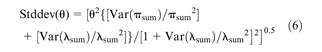
The CMF (θ) is estimated as:

θ = (π_{sum} / λ_{sum}) / {1 + [Var (λ_{sum}) / {λ_{sum}}^{2}]} .

(5)

The standard deviation of θ is given by:

\begin{matrix} Stddev (θ) = [θ^{2} {[Var (π_{sum}) / {π_{sum}}^{2}] \\ + [Var (λ_{sum}) / {λ_{sum}}^{2}]} / [1 + Var (λ_{sum}) / {λ_{sum}}^{2} {]^{2}]}^{0.5} \end{matrix}

(6)

Cross-Sectional Modeling

In this method, crashes are typically assumed to follow a negative binominal (NB) distribution to address overdispersion in crash counts. The treatment and untreated groups are pooled and a dummy variable indicating reference/treatment group is included in the models. The coefficient for this dummy variable is an indicator of the effectiveness of a treatment.

The following example uses the intersection signalized treatment to describe the approach for deriving a CMF from the cross-sectional modes. Suppose a crash prediction model for intersection crashes is the following:

{λ_{i}}_{, t} = α \cdot {ma_aadt}_{i, t}^{β_{1}} {mi_aadt}_{i, t}^{β_{2}} \exp (β_{3} Z + ε_{i})

(7)

and,

${λ_{i}}_{, t}$ = expected number of crashes at intersection $i$ in year $t$

${ma_aadt}_{i, t}$ = annual average daily traffic (AADT) on major road at site $t$ in year $t$

${mi_aadt}_{i, t}$ = AADT on minor road at site $i$ in year $t$

$α = Intercept$

Z = Dummy variable, Z = 1 for treatment site, and Z = 0 for control site

$β_{1}, β_{2}, β_{3} =$ Coefficients for ${ma_aadt}_{i, t}$ , ${mi_aadt}_{i, t}$ , and Z, respectively

The CMF for signalization treatment is exp( $β_{3}$ ). As mentioned earlier, the cross-sectional method is often not able to address the potential bias caused by confounding.

Cross-Sectional along with the PS Matching Methods

Matching is the most common PS method, which involves assembling the treatment sites and the control sites with similar or identical PS. There are many ways to match a control site to a treated site. CMFs can then be estimated from the matched sample. The analysis of the matched samples can then approximate that of a randomized trial by directly comparing outcomes between treatment sites and control sites using methods that account for the paired nature of the data. Examples of such methods include mixed-effect NB or Poisson models based on the matched ID. Many statistical software packages provide options for estimating mixed-effects models; for example, the SAS GLIMMIX procedure can be used to estimate mixed-effects models.

Matching Distances

The first step in matching is selecting the matching distance, that is, which measure(s) should be used to match a control to a treated site. The propensity score distance (PSD) and MD between a treatment and a control sites were used in this study.

PSD

The PS for a treatment can be estimated using binary logistic regression:

\Pr (Z_{i} = 1) | X_{i} = \frac{\exp (β X_{i})}{1 + \exp (β X_{i})}

(8)

where

$\Pr (Z_{i} = 1) | X_{i}$ is the PS for a treatment at site i;

$X_{i}$ is a set of covariates for site i.

$β$ is the vector of parameters associated with covariates $X_{i}$ ;

The absolute value of difference in PS is defined as the PSD and can be used to match treatment site i and control j in the study.

{PSD}_{ij} = | \Pr (Z_{i} = 1) - ⪻ (Z_{j} = 0) |

(9)

MD

MD measures the distance between the two observations X_i in a treatment group and X_j in a control group. The MD is calculated using the following equation.

M D_{ij} = (X_{i} - X_{j})^{'} \sum^{- 1} (X_{i} - X_{j})

(10)

where X_i−X_j is the matrix of the differences in values between treatment site i and control site j for the variables included in the MD calculation, and Σ is the covariance matrix of X between the two groups. It is intuitive to include all the significant variables from the logistic regression for the PS calculation, and for the MD calculation. In addition to all the significant covariates, PS was also included in the MD calculation in this study.

Matching Methods

NN matching with caliper option and the optimal matching are the two most popular and useful methods. In addition, NN match also has options for matching with and without replacement. PSMATCH procedure in SAS 14.2 was used to explore these two matching methods.

Nearest Neighbor (NN) Matching

The NN matching ( 23 ) method is also called Greedy NN matching as it uses a “greedy” algorithm, which cycles through each treated unit one at a time, selecting the available control unit with the smallest distance to the treated site. The algorithm makes “best” matches first and “next-best” matches next, in a hierarchical sequence until no more matches can be made.

1:1 versus k:1 matching

In its simplest form, 1:1 NN matching selects the control site with the smallest distance for each treated site. The advantage for 1:1 matching is that the matched sets are more similar compared with k:1 NN matching. k:1 NN matching allows k controls to be matched to the same treated site. One issue in relation to 1:1 matching is that it can discard many controlled observations and thus may lead to reduced precision for the CMF estimates. On the other hand, although k:1 NN matching increases the matched sample set, it reduces the similarity between the matched treated and control groups. In other words, selecting the number of matches involves a bias-variance trade-off. Selecting multiple controls for each treated site will generally increase bias, as the second, third, and fourth closest matches are further away from the treated site compared with the first closest match. On the other hand, utilizing multiple matches can decrease variance because of the larger matched sample size. An additional concern with k:1 NN matching is that, without any restrictions, it can lead to some poor matches, if for example, there are no control sites with PS similar to a given treated site.

Caliper Width

One strategy to avoid poor matches is to impose a caliper and only select a match if it is within the caliper width. Best matches are those with the lowest matching distances with the range of the caliper width. This can lead to difficulties in interpreting effects if many treated sites do not receive a match, but can help avoid poor matches. For more details, readers are referred to Rosenbaum and Rubin ( 24 ).

With or Without Replacement

One way to resolve the issue when many treated sites do not receive a match is matching with replacements; in other words, one control site could be matched to multiple treated sites based on the aforementioned criteria. Matching with replacement can often decrease bias because controls that look similar to many treated sites can be used multiple times. This is particularly helpful in settings where there are few control sites comparable with the treated sites. However, inference becomes more complex when matching with replacement, because the matched controls are no longer independent. It is also possible that the estimate of the treatment effect will be based on just a small number of controls when matching with replacement.

Optimal Matching

One issue of the NN matching is that the order in which the treated subjects are matched may change the quality of the matches. Optimal matching avoids this issue by taking into account the overall set of matches when choosing individual matches, minimizing a global distance measure ( 25 ). Generally, NN matching performs poorly when there is intense competition for controls, and performs well when there is little competition ( 26 ).

In the SAS PSMATCH procedure, all matches are selected simultaneously and without replacement to minimize the total absolute difference in PS or MD across all matches. Maximum variable ratio allows a specified maximum number of control sites to be matched to each treated site to achieve a minimal global PSD or MD. Note that this option uses much more computer memory compared with the NN matching.

Estimation of CMFs using the PS Matching Methods

For cross-sectional models with the PS matching methods, the CMFs can be derived in two ways:

The CMFs can be estimated in the same way as the traditional cross-sectional method using the NB model. Instead of the whole dataset, the matched datasets are used.

As the matched dataset includes matched treated and control sites, it may be more appropriate to use a method specifically for the matched data, in which treatment effects are estimated after controlling the effects in each of the matched control sites. Mixed-effects model is one of the options for this purpose, in which matched ID is used for the random effects. The Equation for the mixed-effects model is:

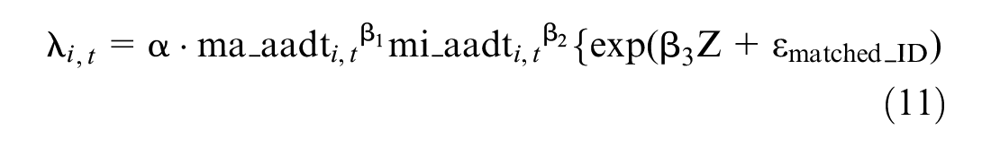
λ_{i, t} = α • m a_a a d t_{i, t}^{β_{1}} m i_a a d t_{i, t}^{β_{2}} \exp (β_{3} Z + ε_{m a t c h e d_I D})

(11)

It can be seen that Equation 11 is similar to Equation 7 for the traditional cross-sectional method. In a mixed-effects model, instead of a site level error $ε_{i}$ , a matched pair error $ε_{matched_ID}$ is used indicating each matched pair share the same error.

Study Design

In simulated datasets the true CMFs are known, and the difference between true and estimated CMFs can be used to assess the reliability of a particular method. Although many studies seek to match the characteristics of treated and untreated sites in before–after as well as cross-sectional studies, treated and untreated sites are often not very similar. Thus, to consider a realistic scenario, the study design should allow for the distribution of the major covariates to be different between the treated and control groups. At the same time, the reference group should have enough sites that can be matched to the treated sites so that it is possible to implement and evaluate the matching methods.

Different true CMF values and overdispersion parameters were used when generating the crash counts. The simulated AADT volumes and crash counts also need to be realistic. For this study, we chose urban stop-controlled intersections as control sites and signalization as a countermeasure. In total 11 years of data were generated, and a signalization treatment was assumed to occur in year 6 at some of the intersections with high traffic volumes on the major road (ma_aadt). The after-period data (i.e., from year 7 to 11) were selected for evaluating the traditional cross-sectional as well as the PS matching methods.

As mentioned earlier, we need to have sufficient number of control sites with similar distributions of the major covariates as the treated group so that the matching methods can be applied. Thus, part of the high AADT intersections was set to be part of the control sites. The majority of the control sites, however, were from the intersections with lower ma_aadt values.

After assigning treatment and control sites and following Donnell et al. ( 16 ), a confounder was then assigned to each treated and control site with different distributions in the two groups. To simulate realistic traffic volumes on major and minor roads as well as crash counts, a literature review was conducted for recent studies on SPFs for urban stop-controlled intersections. The crash counts were then generated for each site assuming a NB distribution using a SPF similar to those found in these previous studies.

Simulated Data

The data used to examine the different methods were generated from a Poisson-Gamma distribution ( 4 , 27 ). The simulation framework for the urban stop-controlled intersection dataset is as follows:

Step 1: For year 1, randomly generated entering traffic volumes on the major road (5000–50,000 ma_aadt) which follows a truncated normal distribution with mean of 20,000 and standard deviation of 6000. Similarly generated AADT on the minor road (500–5,000 mi_aadt) with mean of 2,000 and standard deviation of 600. The number of sites was set to be 100,000 to ensure that enough control sites can be obtained that are significantly different from the treated sites in relation to ma_aadt.

Step 2: ma_aadt and mi_aadt for the remaining 10 years were generated with random variation (within 5%), such that most of the traffic volumes would be around the mean value 20,000 and 2,000, respectively.

Step 3: Sorted the ma_aadt from high to low. Then randomly assigned 5%–20% of the top 3,000, 5,000, and 10,000 high ma_aadt sites to be treated sites. The remaining sites with high ma_aadt values were partially assigned to the control group. The number of the assigned control sites with high ma_aadt values was about 2–6 times the treated sites. Multiple datasets were generated at this step.

Step 4: 20,000–30,000 sites with the lowest ma_aadt values in the initially generated 100,000 sites were added to the control group.

Step 5: Generated a confounding variable v_w with different distribution between the treated and control groups.

v_w | Z ~ N (50^{*} (1 + 0.5 Z), {(10^{*} (1 + 0.5 Z))}^{2})

(12)

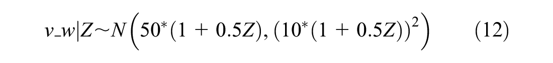
where

Z=Dummy variable, Z=1 for treatment site, and Z=0 for control site

Step 6: As mentioned earlier, year 6 was assumed to be the treatment year. Year 1 through year 5 is the before period and years 7 through 11 is the after period. CMFs were applied to treated sites in the after period when generating the crash counts from the NB models, based on the following model.

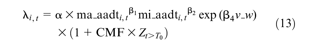
\begin{matrix} {λ_{i}}_{, t} = & α \times {ma_aadt}_{i, t}^{β_{1}} {mi_aadt}_{i, t}^{β_{2}} \exp (β_{4} v_w) \\ \times (1 + CMF \times Z_{t > T_{0}}) \end{matrix}

(13)

where

$β_{4}$ = parameter associated with the confounding variable v_w,

$Z_{t > T_{0}}$ = dummy variable, $Z_{t > T_{0}}$ =1 for treated sites when year > treatment year T₀; otherwise $Z_{t > T_{0}}$ = 0.

Crash counts were generated based on SPFs from previous studies. Specifically, parameters $α$ , $β_{1}, β_{2}$ were assumed based on the SPFs from California ( 28 ) and Virginia ( 29 ). The used SPF was:

\begin{matrix} {λ_{i}}_{, t} = & 0.00004 \times {ma_aadt}_{i, t}^{0.6191} {mi_aadt}_{i, t}^{0.4813} \\ \exp (0.015 v_w) \times (1 + CMF \times Z_{t > T_{0}}) \end{matrix}

(14)

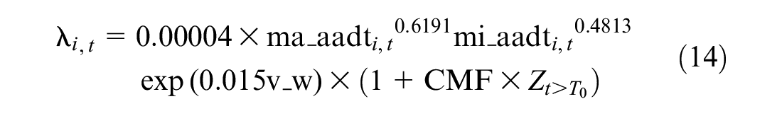
where CMF is assumed to be 1.3 and 1.0, respectively for the above datasets.

Step 7: Calculated the expected number of crashes ${λ_{i}}_{, t}$ for intersection $i$ across 11 years from the above SPF (Equation 14).

Step 8: Generated a scale factor $δ_{i}$ from a Gamma distribution with the mean equal to 1 and the over dispersion parameter φ: $δ_{i} ~ gamma (ϕ, \frac{1}{ϕ})$

Step 9: Calculated the modified mean ${μ_{i}}_{, t} = λ_{i, t} \times δ_{i}$

Step 10: Generated observed crash counts ( $Y_{i, t}$ ) at intersection $i$ in year $t$ from a Poisson distribution with mean ${μ_{i}}_{, t}$ .

For the generated datasets, the EB before–after evaluation and traditional cross-sectional analysis were conducted. The final simulated datasets were selected such that the characteristics of the treated and control sets were significantly different, which led to the estimated CMFs from the EB method to be significantly different from the true CMF—the intent was to determine whether the PS method would provide an estimated CMF that was closer to the true CMF compared with the EB method. The final two simulated datasets and their summary statistics are described in Table 1. It is clear that the ma_aadt and average crashes per site per year in the treated group are higher than those in the reference group, as expected.

Table 1.

Summary Statistics for Simulated Dataset 1 and 2

	Dataset 1:True CMF = 1.30, dispersion parameter = 1/1.5					Dataset 2:True CMF = 1.00, dispersion parameter = 2
Variable	Control/treated	Min	Max	Mean	SD	Control/treated	Minimum	Maximum	Mean	SD
confounding variable v_w	Control group 21000 sites (1000 sites with high ma_aadt)	8.25	90.58	50.06	10	Control group 23000 sites (3000 sites with high ma_aadt)	11.3	89.74	49.97	9.94
ma_aadt		11219	47528	15712	4807		8998	47528	16049	7115
mi_aadt		485	5273	1963	597		487	5273	1967	618
Crashes/site.year		0	12.91	1.29	3.99		0	31.73	1.28	6.61
ma_aadt - before		10122	47818	15790	4659		8185	47818	16063.4	6891.79
mi_aadt - before		491	4956	1963	591		496	4956	1967.03	612.05
ma_aadt - after		12018	51087	15636	5002		9727	51087	16035.29	7369.87
mi_aadt - after		462	5560	1963	608		462	5560	1966.55	628.78
Crashes/site.year - before		0	12.2	1.3	2.83		0	31.6	1.29	4.53
Crashes/site.year - after		0	14.6	1.28	2.81		0	34	1.28	4.55
confounding variable v_w	Treated group 386 sites	26.05	117.53	76.39	14.61	Treated group 343 sites	31.63	115.94	74.91	14.07
ma_aadt - before	Treated group 386 sites	26782	43712	31854	2671	Treated group 343 sites	24439	40561	30202	2733
mi_aadt - before		589	4507	2126	684		681	3860	2104	623
ma_aadt - after		30469	46245	33138	2423		28057	41851	31136	2601
mi_aadt - after		556	4341	2124	696		654	3887	2109	641
Crashes/site.year - before		0	16	3.19	6.14		0	33.6	3.35	11.06
Crashes/site.year - after		1	19	4.65	8.02		0	36.8	3	10.94

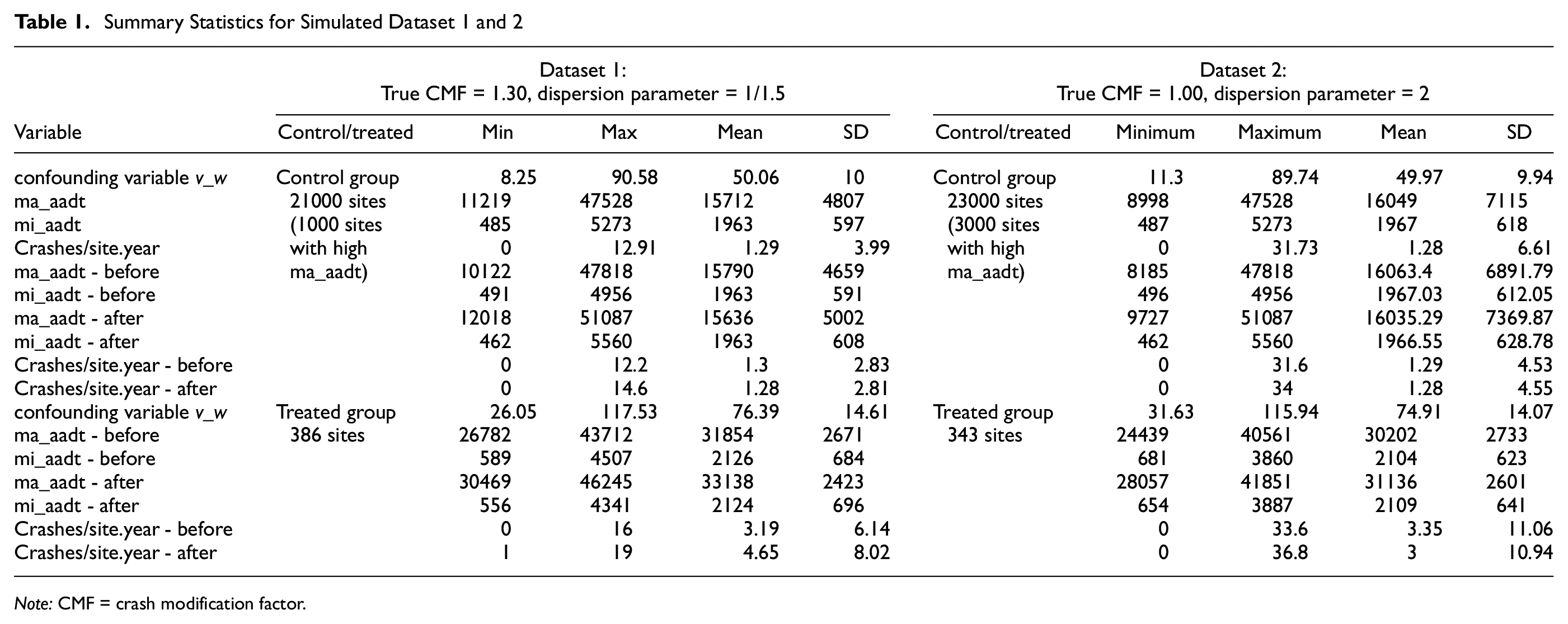
Note: CMF = crash modification factor.

Evaluation Results

The two simulated datasets were explored using the EB, traditional cross-sectional, and the various PS methods as aforementioned. The NN PSD matching was explored with 5 replacements and MD match using 1, 5, and 10 replacements, respectively. The optimal matching by PSD and MD was also investigated, and the maximum variable ratio was set to be 5.

CMFs from Dataset 1

There are 386 treated sites and 21,000 reference sites in dataset 1 and the true CMF=1.30. Among the 21,000 reference sites, there are 1,000 sites with ma_aadt values similar to those in the treated sites and 20,000 sites with much lower ma_aadt values. The CMFs in relation to mean and 95% confidence limits by various methods are shown in Table 2.

Table 2.

Comparison of CMFs for Dataset 1 (True CMF = 1.30)

CMF	CMF 95% confidence limits		Method	Model	Control sites	Treated sites	CMF correctly identified?
1.427	1.382	1.473	EB	NB	21000	386	No
1.399	1.328	1.473	Traditional Cross-Sectional	NB	21000	386	No
0.674	0.521	0.872	NN matching by PSD (5 replacements)	NB	10	371	No
0.602	0.515	0.703	NN matching by PSD (5 replacements)	Mixed-effects Poisson	10	371	No
1.391	1.232	1.571	NN matching by MD (1 replacement)	NB	58	362	Yes
1.289	1.170	1.420	NN matching by MD (5 replacements)	NB	198	362	Yes
1.262	1.158	1.375	NN matching by MD (5 replacements)	Mixed-effects NB	198	362	Yes
1.328	1.212	1.454	NN matching by MD (10 replacements)	NB	313	362	Yes
1.302	1.233	1.375	NN matching by MD (10 replacements)	Mixed-effects Poisson	313	362	Yes
1.331	1.240	1.428	Optimal matching by PSD (max variable ratio=5)	NB	1158	386	Yes
1.358	1.296	1.423	Optimal matching by PSD (max variable ratio=5)	Mixed-effects Poisson	1158	386	Yes
1.364	1.276	1.459	Optimal matching by MD (max variable ratio=5)	NB	1158	386	Yes
1.463	1.391	1.538	Optimal matching by MD (max variable ratio=5)	Mixed-effects Poisson	1158	386	No

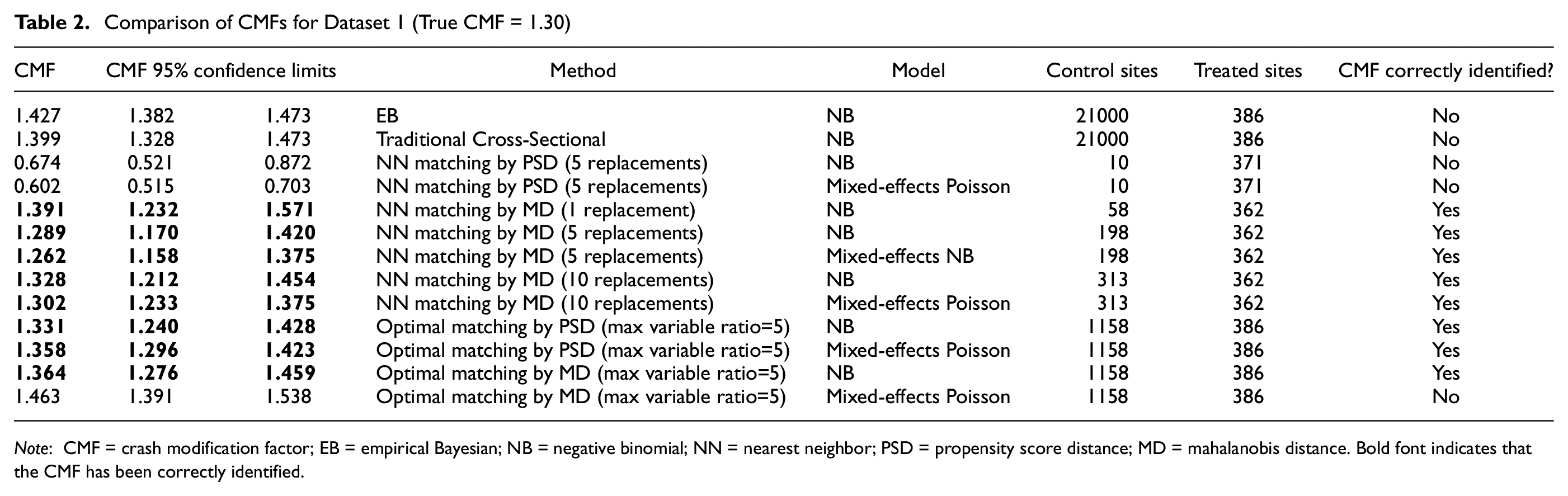
Note: CMF = crash modification factor; EB = empirical Bayesian; NB = negative binomial; NN = nearest neighbor; PSD = propensity score distance; MD = mahalanobis distance. Bold font indicates that the CMF has been correctly identified.

If the true CMF 1.30 is located between the 95% confidence limits of the estimated CMFs, we concluded that the method correctly identifies the true effects and reported a “Yes” in Table 2. Otherwise, we reported a “No”.

For the EB and traditional cross-sectional methods, the 95% confidence intervals of the estimated CMFs did not include the true CMF value. The NN PSD matching with 5 replacements had the worst results because only 10 control sites were repeatedly matched to the 371 treated sites. All other matching methods, except optimal matching by MD using the mixed-effects model, correctly identify the true effects. It can be seen the CMFs from the mixed-effects models are generally consistent with those from the NB models, but with a lower standard error. The lower standard error means a more stable estimate. Thus the mixed-effects model seems to be a better option for the CMF estimation for the matching methods. The CMFs from the mixed-effects Poisson models are listed in Table 3, whereas the mixed-effects NB models did not converge.

Table 3.

Comparison of CMFs for Dataset 2 (True CMF = 1.00)

CMF	CMF 95% confidence limits		Method	Model	Control sites	Treated sites	CMF correctly identified?
0.884	0.851	0.917	EB	NB	23000	343	No
1.016	0.938	1.100	Traditional cross-sectional	NB	23000	343	Yes
0.656	0.235	1.831	NN matching by PSD (5 replacements)	NB	5	341	No
0.654	0.239	1.790	NN matching by PSD (5 replacements)	Mixed-effects NB	5	341	No
1.057	0.873	1.282	NN matching by MD (1 replacement)	NB	101	343	Yes
1.012	0.942	1.087	NN matching by MD (1 replacement)	Mixed-effects Poisson	101	343	Yes
1.137	0.995	1.301	NN matching by MD (5 replacements)	NB	311	343	No
1.123	0.989	1.276	NN matching by MD (5 replacements)	Mixed-effects NB	311	343	No
1.195	1.139	1.254	NN matching by MD (10 replacements)	NB	509	343	No
1.182	1.050	1.331	NN matching by MD (10 replacements)	Mixed-effects NB	509	343	No
1.035	0.910	1.177	Optimal matching by PSD (max variable ratio=5)	NB	1029	343	Yes
0.991	0.934	1.051	Optimal matching by PSD (max variable ratio=5)	Mixed-effects Poisson	1029	343	Yes
1.149	1.037	1.272	Optimal matching by MD (max variable ratio=5)	NB	1029	343	No
1.234	1.188	1.281	Optimal matching by MD (max variable ratio=5)	Mixed-effects Poisson	1029	343	No

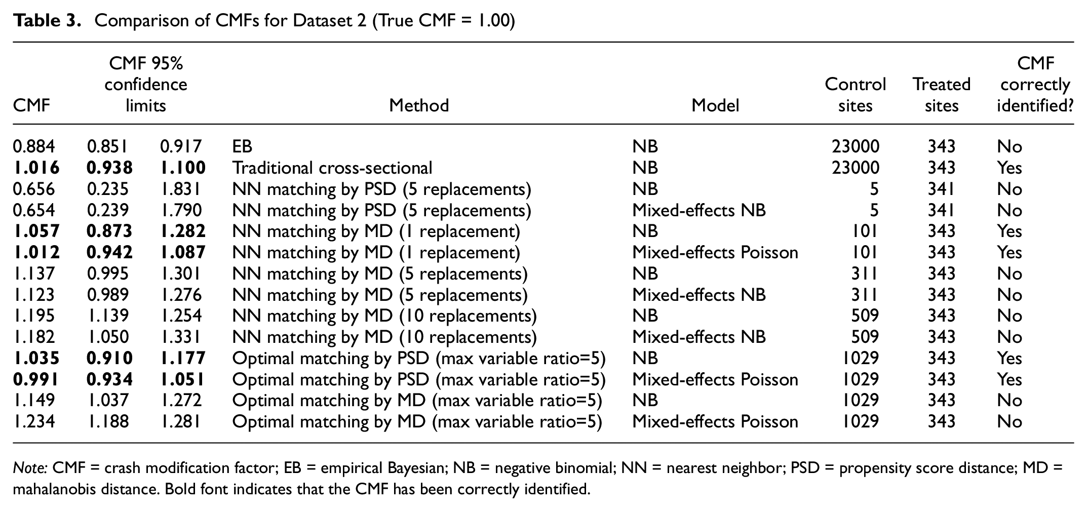
Note: CMF = crash modification factor; EB = empirical Bayesian; NB = negative binomial; NN = nearest neighbor; PSD = propensity score distance; MD = mahalanobis distance. Bold font indicates that the CMF has been correctly identified.

Figure 1 illustrates the pattern of the standardized mean differences (SMD) for PS, Logit propensity score (LPS), the confounding variable v_w, and the logarithm value of average ma_aadt in the after period from year 7 to year 11 (lnma7_11m) matched by the NN PSD and MD with 5 replacements, respectively. The SMD is computed by dividing the mean difference (Treated – Control) by an estimate of the standard deviation. SMD can be used to show the quality of the matching—if the absolute value of SMD is closer to 0, there is better balance in the treated and control groups. Note that mi_aadt is not significant in the logistic regression, and not shown in Figure 1.

Figure 1.

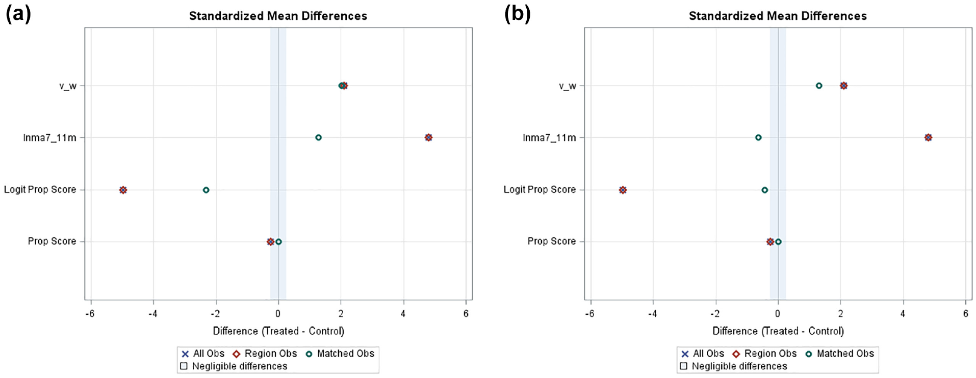
Standardized mean differences from NN matching by PSD and MD (a) NN matching by PSD, and (b) NN matching by MD.

“All Obs” in the legend in Figure 1 stands for all the data, and “Region Obs” is the data where PS are in the common support region. The common support region is also the largest interval that contains PS for subjects in both groups. “Matched Obs” refers to the matched data.

For the NN PSD matching in Figure 1a, the SMD of zero for the PS in the matched data is expected as PSD was the matching criterion. SMD for the LPS and lnma7_11m are much smaller than those in the original or the common region data, indicating these variables are better balanced in the matched data. The SMD for the confounding variable v_w is almost the same as before matching; this is expected, as we purposely implemented the different means for v_w into the two groups. In Figure 1b, for the NN MD matching with 5 replacements, the absolute value of the SMDs are much smaller than those matched by PSD, implying that the variables in the treated and control groups are much better balanced compared with the NN PSD matching.

Note that zero of SMD in Figure 1 cannot be interpreted as a perfect match as it is only about the mean difference. To better understand the balance of the variables in the matched data, we can take a look at the boxplots of lnma7_11m in Figure 2. It can be seen the balance of this variable is much more improved by NN MD matching in Figure 2b. lnma7_11m in Figure 2a has a much wider range in the matched control group compared with the treated group, indicating a poor match. Since ma_aadt is a major factor associated with the crashes, NN PSD had the worst results. Only 10 control sites are in the matched data.

Figure 2.

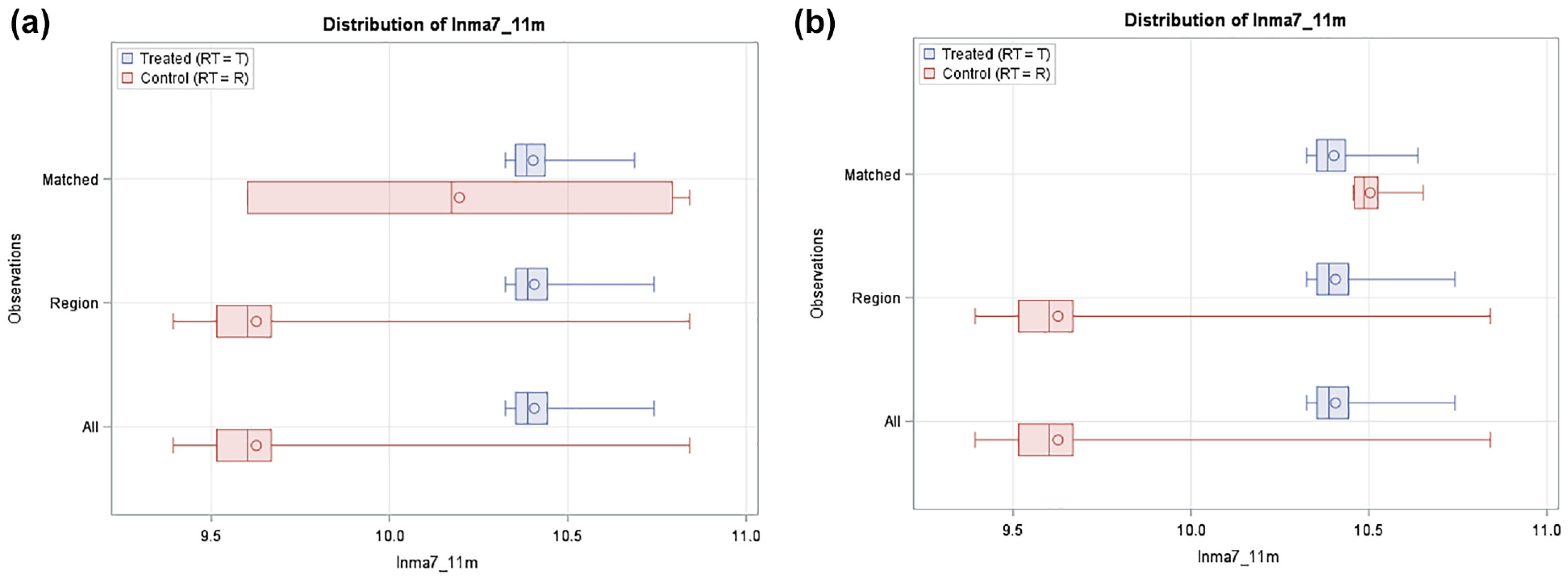
Distribution of lnma7_11m from NN matching by PSD and MD (a) NN matching by PSD, and (b) NN matching by MD.

From Table 2, surprisingly, the CMFs by the optimal matching using MD is not as good as the CMFs by the optimal PSD matching. For the latter method, the objective function is to have a minimal absolute difference of PS. In Figure 3, the SMD point for PS is not located near the zero line as the two NN matching methods. The reason is, unlike RMSE, the SMD is about the mean difference. Although the SMD graph for optimal PSD is not as good as the one by the NN MD method in Figure 1b, the boxplots in Figure 4 show the balance for variable lnma7_11 are as good as those by the NN MD. The number of matched control sites by this method is 1,158 whereas it is just 198 by the NN MD method. A larger sample size of the control group allows a smaller standard error of CMF as shown in Table 2. Given the similar CMF values by the two methods, the optimal matching by PSD is better because of a smaller standard error of the CMF estimates.

Figure 3.

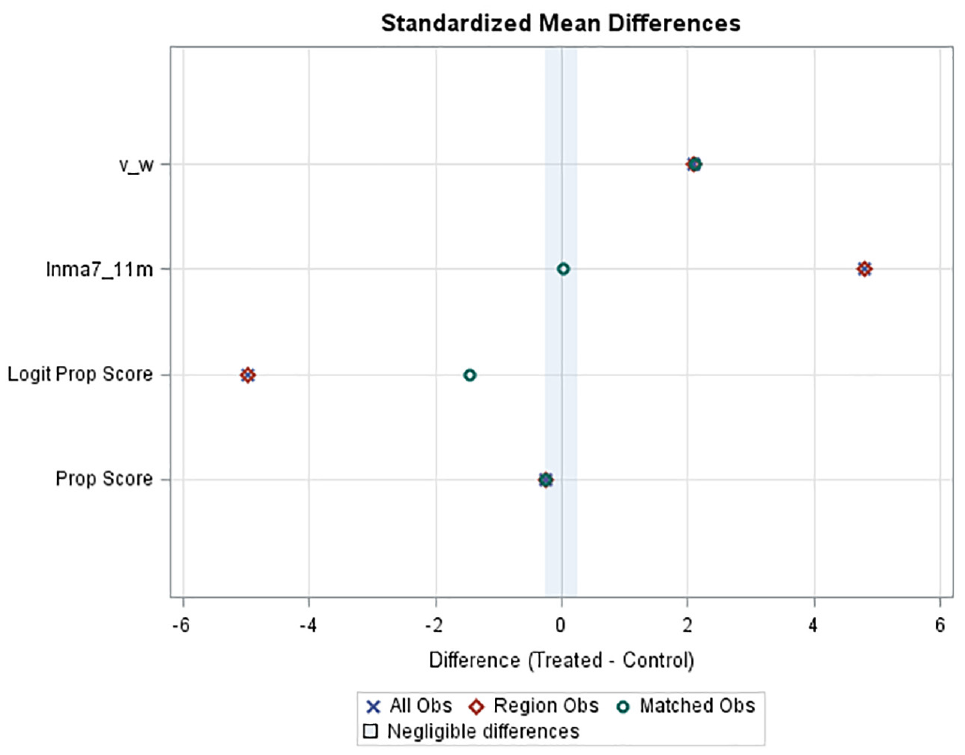
Standardized mean differences from optimal matching by PSD.

Figure 4.

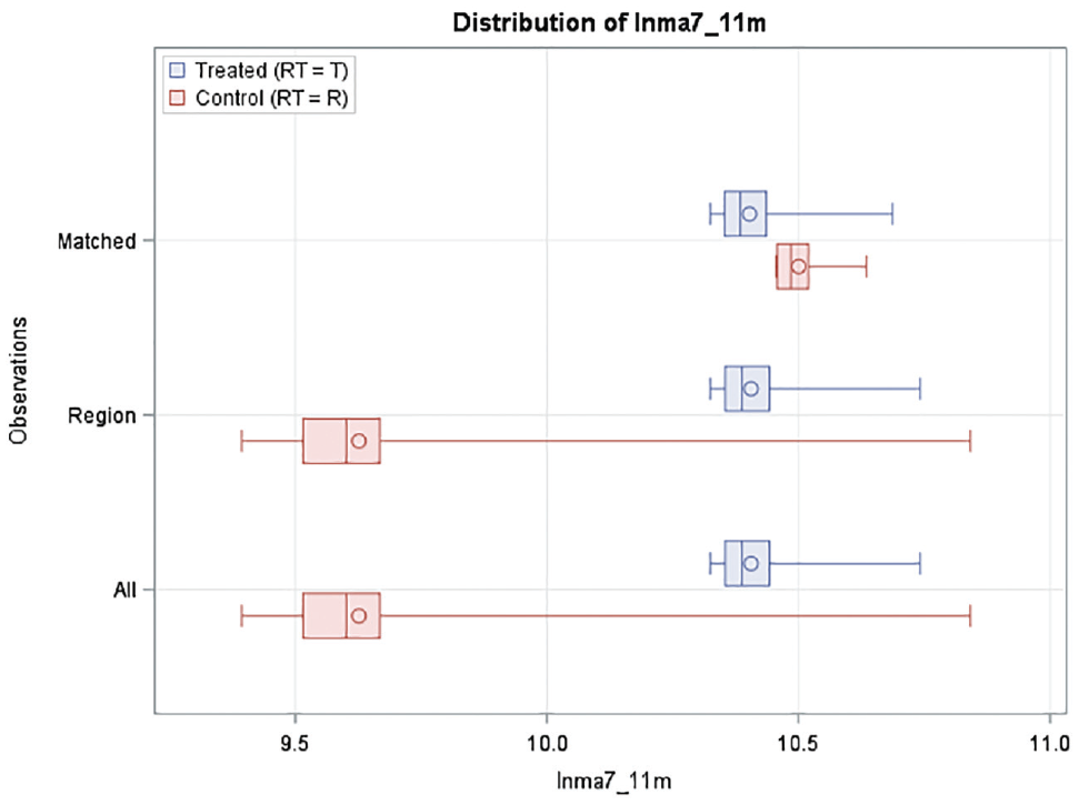
Distribution of lnma7_11m from optimal matching by PSD.

CMFs from Dataset 2

The dataset 2 has 343 treated sites and 23,000 control sites, and its true CMF is 1.00. The CMF results are in Table 3. NN PSD matching continues to have least matched control sites (5 sites only) and provides the poorest CMF estimates. On the other hand, optimal PSD matching continues to provide the most promising CMFs estimates. In addition, NN MD matching with 1 or 5 replacements also correctly estimates the true effects. The matching with 1 replacement has better estimates than the matching with 5 replacements. Surprisingly, the traditional cross-sectional method also correctly estimates the true CMF. Again, the optimal MD matching does not perform well.

Two statistical measures for balance assessment, which are the SMD between the treatment and control groups and the treated-to-control variance ratio, are listed in Table 4. The variance ratio is calculated by dividing the variance in the treated group by the variance in the control group for each variable. For good variable balance, the absolute standardized mean difference should be less than or equal to 0.25, and the variance ratio should be between 0.5 and 2 ( 30 ).

Table 4.

Variable Balance Information in the Matched Data

Matching method	Variable	Observations	Mean difference	Standard deviation	Standardized mean difference	Variance ratio
NN matching by PSD with 5 replacements	lnma7_11m	All	0.7326	0.2511	2.917	0.053
		Region	0.7326	na	2.917	0.053
		Matched	0.8044	na	3.203	na
	v_w	All	24.9439	12.1828	2.047	2.006
		Region	24.9439	na	2.047	2.006
		Matched	21.5501	na	1.769	3.251
Optimal matching by PSD with max. variable ratio of 5	lnma7_11m	All	0.7326	0.2511	2.917	0.053
		Region	0.7326	na	2.917	0.053
		Matched	–0.1343	na	–0.535	0.125
	v_w	All	24.9439	12.1828	2.047	2.006
		Region	24.9439	na	2.047	2.006
		Matched	25.5264	na	2.095	2.027

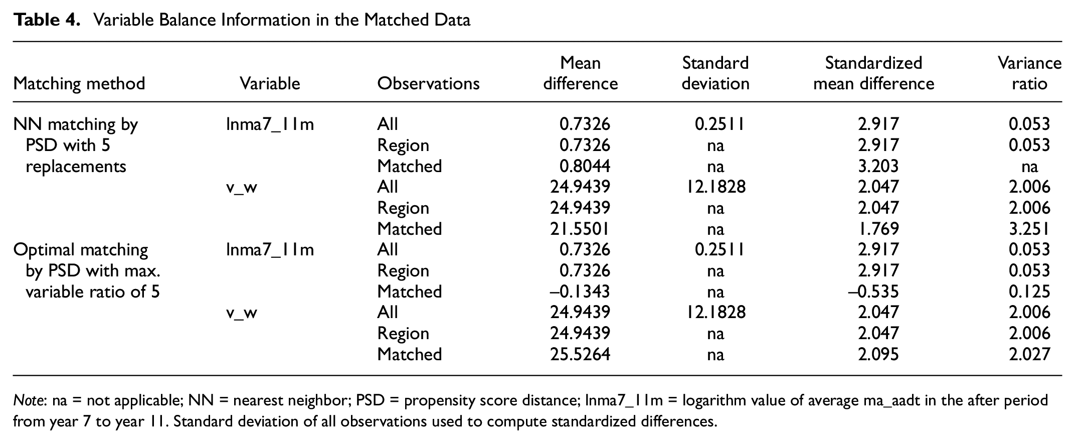
Note: na = not applicable; NN = nearest neighbor; PSD = propensity score distance; lnma7_11m = logarithm value of average ma_aadt in the after period from year 7 to year 11. Standard deviation of all observations used to compute standardized differences.

The two statistical measures for v_w and lnma7_11m for NN PSD with 5 replacements and optimal PSD matching are shown in Table 4. The SMD for lnma7_11m is getting larger after NN PSD matching. This indicates that the balance of this variable is becoming worse after matching. The SMD for v_w becomes smaller after match, but the variance ratio is getting bigger and far away from 2. It is not clear if the balance for v_w is indeed improved based on the conflicting information in the SMD and the variance ratio.

After the optimal PSD matching, the SMD is significantly reduced from 2.9 to –0.53 and the variance ratio is also improved for variable lnma7_11m, indicating the balance of lnma7_11m is greatly improved after matching. Distribution of v_w is almost the same as in the original data. The CMFs from the optimal PSD match are almost identical to the true CMF.

Comparison of the Methods

From Tables 2 and 3, we can see the CMFs from the two datasets are not always consistent. Out of 14 methods or options, only three of them can consistently correctly identify the true effects using the two simulated datasets. The three methods are the optimal PSD matching with max variable ratio of 5 with NB or mixed-effects model, and the NN MD matching with 1 replacement using the NB model. The CMFs identified by the optimal PSD matching are much better than those by the NN MD matching with 1 replacement in relation to being closer to the true CMFs, and having lower standard errors.

Discussion

There are other methods that have been used to address confounding when using the cross-sectional method to estimate CMFs. The case-control method is one example of such a method. One of the most important steps in a case-control study is defining the cases and controls. Ambiguous or broad definitions for cases and controls may lead to misclassification and will likely produce unreliable results. Care must be taken to ensure that cases and controls are representative of the sites of interest ( 31 ). This may be difficult, as each risk factor may affect crashes in different ways. Perfect matching on the risk factors in the treatment and control groups is very difficult, and probably impossible.

Confounding issue may cause biased CMF estimates even when using the before–after method ( 32 ). Reference sites are needed for the EB method. As indicated by Elvik, it is not always obvious which confounding factors are controlled for by using a comparison group ( 32 ). If there are strong confounding variables used to select the treatment, in other words, if one or more important risk factors are significantly different in the reference and treatment groups, the EB-estimated CMFs will be biased. The CMFs estimated by the EB method will be improved had the matched sample been used instead in this case.

Simulation studies have many advantages when comparing the performance of different statistical methods in an efficient manner. For this reason, statisticians often use simulated data when comparing different methods ( 33 ). At the same time, the reliability of a simulation study is dependent on the assumptions that are used in developing the simulated data. It is very difficult for a simulated dataset to completely mimic a complex realistic situation, although recent research using artificial realistic data has come close ( 34 ).The authors feel that simulation was appropriate for this study because true CMFs would not be known if using the real data. In addition, simulated crash counts were generated from the SPFs that were in turn based on real data. So, the authors feel that the simulated crash counts are reasonable.

Conclusion

The cross-sectional along with various PS matching methods were explored. These methods were evaluated and compared with the two most common CMF evaluation methods—the traditional cross-sectional and the EB before–after methods using two carefully selected simulated datasets. The important findings are:

The NN MD matching with 1 replacement and the optimal PSD matching with max variable ratio of 5 correctly identify the true effects.

The optimal PSD matching with max variable ratio of 5 has the greatest number of matched control sites and provides the best CMF estimates.

The NN PSD matching with 5 replacements has the least number of matched control sites and is the worst method for CMF estimates.

The optimal MD matching with max variable ratio of 5 does not perform as well as the NN MD matching with 5 replacements.

The mixed-effects model has better results than the traditional NB models in relation to providing better estimates for the mean values and smaller standard errors.

Based on the findings, we recommend the optimal PSD matching for the evaluation of CMFs. It can be seen the optimal PSD is better than the EB method, in that the EB method fails to identify the true effects. However, it is worth mentioning that only the reference sites were used to develop the SPFs in the EB method. There are other techniques for the EB; for example, in some cases when the treated and reference sites are very different, the treated group in the before-period data has been used for SPF development ( 35 ). Future research could explore the performance of the EB method using matched datasets. Moreover, as the two datasets were specifically selected where the EB method failed to identify the true effects, it may be premature to conclude that the recommended optimal PSD method is better than the EB method for CMF evaluations, but the optimal PSD method does provide some promise. More simulation studies are needed to confirm the findings in this study. In addition, other PS options such as PS weighting should be explored in future studies.

Although there have been a few CMF evaluations using the PS matching methods for road safety studies, to the authors’ knowledge, the recommended optimal PSD matching method has not been used in road safety studies. It is our hope that this study provides useful insights that could be used for better CMF evaluations.

Footnotes

Author Contributions

The authors confirm contribution to the paper as follows: study conception and design: Bo Lan, Raghavan Srinivasan; analysis and interpretation of results: Bo Lan; draft manuscript preparation: Bo Lan. All authors reviewed the results and approved the final version of the manuscript.

Declaration of Conflicting Interests

The author(s) declared no potential conflicts of interest with respect to the research, authorship, and/or publication of this article.

Funding

The author(s) disclosed receipt of the following financial support for the research, authorship, and/or publication of this article: This research was funded by the Southeastern Transportation Center that was part of Region 4 of the University Transportation Center (UTC).

References

Federal Highway Administration. Crash Modification Factors in Practice. Report FHWA-SA-13-017. 2014. http://safety.fhwa.dot.gov/tools/crf/resources/cmfs/docs/product_summary_final.pdf.

Hauer

Observational Before-After Studies in Road Safety: Estimating the Effect of Highway and Traffic Engineering Measures on Road Safety. Pergamon Press, Elsevier Science Ltd, Oxford, 1997.

Sacchi

Sayed

Investigating the Accuracy of Bayesian Techniques for Before-After Safety Studies: The Case of a “No Treatment” Evaluation. Accident Analysis and Prevention, Vol. 78, 2015, pp. 138–145.

Lan

Persaud

Lyon

Bhim

Validation of a Full Bayes Methodology for Observational Before–After Road Safety Studies and Application to Evaluation of Rural Signal Conversions. Accident Analysis & Prevention, Vol. 41, No. 3, 2009, pp. 574–580.

Persaud

Lan

Lyon

Bhim

Comparison of Empirical Bayes and Full Bayes Approaches for Before–After Road Safety Evaluations. Accident Analysis & Prevention, Vol. 42, No. 1, 2010, pp. 38–43.

Hauer

Cause, Effect and Regression in Road Safety: A Case Study. Accident Analysis and Prevention, Vol. 42, No. 4, 2010, pp. 1128–1135.

Hauer

Enhancing Future CMF Research. Working Paper, 2016. https://www.researchgate.net/publication/292607664_Enhancing_future_CMF_research.

Hauer

Even Perfect Regressions may not Tell the Effect of Interventions. Proc., Transportation Research Board Annual Conference, Washington D.C., 2013.

Gross

Persaud

Lyon

A Guide to Developing Quality Crash Modification Factors. Report FHWA-SA-10-032. Federal Highway Administration, Washington, D.C., 2010.

10.

Carter

Srinivasan

Gross

Council

NCHRP Project 20-07/Task 314: Recommended Protocols for Developing Crash Modification Factors. Transportation Research Board of the National Academies, Washington, D.C., 2012.

11.

Miaou

S. P.

Lum

Modeling Vehicle Accidents and Highway Geometric Design Relationships. Accident Analysis and Prevention, Vol. 25, No. 6, 1993, pp. 689–709.

12.

Donnell

E. T.

Porter

R. J.

Shankar

V. N.

Framework for Assessing the Safety Effects of Roadway Lighting. Safety Science, Vol. 48, No. 10, 2010, pp. 1436–1444.

13.

Donnell

E. T.

Gross

Case-Control and Cross-Sectional Methods for Estimating Crash Modification Factors: Comparisons from Roadway Lighting and Lane and Shoulder Width Safety Effect Studies. Journal of Safety Research, Vol. 42, No. 2, 2011, pp. 117–129.

14.

Austin

P. C.

An Introduction to Propensity Score Methods for Reducing the Effects of Confounding in Observational Studies. Multivariate Behavioral Research, Vol. 46, No. 3, 2011, pp. 399–424.

15.

Rosenbaum

P. R.

Rubin

D. B.

Assessing Sensitivity to an Unobserved Binary Covariate in an Observational Study with Binary Outcome. Journal of the Royal Statistical Society Series B (Methodological), Vol. 45, No. 2, 1983, pp. 212–218.

16.

Donnell

Hanks

Porter

R. J.

Cook

Srinivasan

Nguyen

Eccles

Project A-6: Highway Safety Statistical Paper Synthesis. Federal Highway Administration, Washington, D.C., 2017.

17.

Sasidharan

Donnell

E. T.

Application of Propensity Scores and Potential Outcomes to Estimate Effectiveness of Traffic Safety Countermeasures: Exploratory Analysis using Intersection Lighting Data. Accident Analysis and Prevention, Vol. 50, 2013, pp. 539–553.

18.

Wood

J. S.

Gooch

J. P.

Donnell

E. T.

Estimating the Safety Effects of Lane Widths on Urban Streets in Nebraska using the Propensity Scores-Potential Outcomes Framework. Accident Analysis and Prevention, Vol. 82, 2015, pp. 180–191.

19.

Highway Safety Manual. American Association of State Highway and Transportation Officials, Washington, D.C., 2010.

20.

Wood

J. S.

Donnell

E. T.

Safety Evaluation of Continuous Green T Intersections: A Propensity Scores-Genetic Matching-Potential Outcomes Approach. Accident Analysis and Prevention, Vol. 93, 2016, pp. 1–13.

21.

Wood

J. S.

Donnell

E. T.

Porter

R. J.

Comparison of Safety Effect Estimates Obtained from Empirical Bayes Before–After Study, Propensity Scores-Potential Outcomes Framework, and Regression Model with Cross-Sectional Data. Accident Analysis and Prevention, Vol. 75, 2015, pp. 144–154.

22.

Hauer

Harwood

D. W.

Council

F. M.

Griffith

M. S.

Estimating Safety by the Empirical Bayes Method: A Tutorial. Transportation Research Record: Journal of the Transportation Research Board, 2002. 1784: 126–131.

23.

Rubin

D. B.

Matching to Remove Bias in Observational Studies. Biometrics, Vol. 29, No. 1, 1973, pp. 159–183.

24.

Rosenbaum

P. R.

Rubin

D. B.

The Bias due to Incomplete Matching. Biometrics, Vol. 41, No. 1, 1985, pp. 103–116.

25.

Rosenbaum

P. R.

Observational Studies, 2nd ed. Springer-Verlag, New York, NY, 2002.

26.

X. S.

Rosenbaum

P. R.

Comparison of Multivariate Matching Methods: Structures, Distances, and Algorithms. Journal of Computational and Graphical Statistics, Vol. 2, No. 4, 1993, pp. 405–420.

27.

Lord

Modeling Motor Vehicle Crashes using Poisson-Gamma Models: Examining the Effects of Low Sample Mean Values and Small Sample Size on the Estimation of the Fixed Dispersion Parameter. Accident Analysis and Prevention, Vol. 38, No. 4, 2006, pp. 751–766.

28.

Bhim

Observational Before and After Safety Study of Installing Signals at Rural Intersections: Using the Empirical Bayes (EB) and Conventional Methods. Ryerson University, 2006.

29.

Garber

N. J.

Rivera

Safety Performance Functions for Intersections on Highways Maintained by the Virginia Department of Transportation. Final Contract Report VTRC 11-CR1. Virginia Transportation Research Council, Charlottesville, 2010.

30.

Rubin

D. B.

Using Propensity Scores to Help Design Observational Studies: Application to the Tobacco Litigation. Health Services and Outcomes Research Methodology, Vol. 2, No. 3–4, 2001, pp. 169–188.

31.

Gross

Persaud

Lyon

A Guide to Developing Quality Crash Modification Factors. Report No. FHWA-SA-10-032. Federal Highway Administration, Washington, D.C., 2010. http://www.cmfclearinghouse.org/collateral/CMF_Guide.pdf.

32.

Elvik

The Importance of Confounding in Observational Before-and-After Studies of Road Safety Measures. Accident Analysis and Prevention, Vol. 34, No. 5, 2002, pp. 631–635.

33.

Morris

T. P.

White

I. R.

Crowther

Using Simulation Studies to Evaluate Statistical Methods. Statistics in Medicine, Vol. 38, No.11, 2017, pp. 2074–2102.

34.

Srinivasan

Estimation of Crash Modification Factors with Cross-Sectional Data: An Investigation using a Simulated Artificial Realistic Dataset. Proc., Road Safety Simulation Conference, The University of Iowa, 2019.

35.

Persaud

Lyon

Empirical Bayes Before-After Studies: Lessons Learned from Two Decades of Experience and Future Directions. Accident Analysis and Prevention, Vol. 39, No. 3, 2007, pp. 546–555.

Comparison of Crash Modification Factors for Engineering Treatments Estimated by Before–After Empirical Bayes and Propensity Score Matching Methods

Abstract

Summary of Recent Studies in Traffic Study using the Propensity Score Methods

Study Objective and Overview of Approach

Methods Explored

The EB Method

Cross-Sectional Modeling

Cross-Sectional along with the PS Matching Methods

Matching Distances

PSD

MD

Matching Methods

Nearest Neighbor (NN) Matching

Optimal Matching

Estimation of CMFs using the PS Matching Methods

Study Design

Simulated Data

Evaluation Results

CMFs from Dataset 1

CMFs from Dataset 2

Comparison of the Methods

Discussion

Conclusion

Footnotes

Author Contributions

Declaration of Conflicting Interests

Funding

References