Sage Journals: Discover world-class research

Abstract

Detector data can be used to construct cumulative flow curves, which in turn can be used to estimate the traffic state. However, this approach is subject to the cumulative error problem. Multiple studies propose to mitigate the cumulative error problem using probe trajectory data. These studies often assume “no overtaking” and thus that the cumulative flow is zero over probe trajectories. However, in multi-lane traffic this assumption is often violated. Therefore, we present an approach to estimate the change in cumulative flow along probe trajectories between detectors based on disaggregated detector data. The approach is tested with empirical data and in microsimulation. This shows that the approach is a clear improvement over assuming “no overtaking” in free-flow conditions. However, the benefits are not clear in varying traffic conditions. The approach can be applied in practice to mitigate the cumulative error problem and estimate the traffic state based on the resulting cumulative flow curves. As the performance of the approach depends on the changes in traffic conditions, it is suggested to use the probe speed observations between detectors to assign an uncertainty to the change in cumulative flow estimates. Furthermore, a potential option for future work is to use more elaborate schemes to estimate the probe relative flow between detectors, which may, for instance, combine probe speeds with estimates of the macroscopic states along the probe trajectory. If these macroscopic estimates are based on the cumulative flow curves at the detector locations, this would result in an iterative approach.

Traffic state estimation (TSE) is important in dynamic traffic management (DTM) applications ( 1 ). TSE aims to infer the traffic state (which may be described using different variables) from incomplete and inaccurate information, for example, partially observed and noisy traffic-sensing data and traffic-flow models. The traffic state estimates can be used as input for different types of DTM applications, for example, local ramp-metering ( 2 ) or network-wide traffic management ( 3 ).

Throughout this study, road segments without discontinuities (which are denoted as links) are considered. In these links, the conservation-of-vehicles condition holds. Vehicles enter (flow in) the link at the upstream boundary and leave (flow out) the link at the downstream boundary.

Traffic can be described using three dimensions: space $x$ , time $t$ , and cumulative flow $N$ ( 4 ). The cumulative flow $N (x, t)$ denotes the number of vehicles that have passed position $x$ at time $t$ . Here, it is important that the same set of vehicles is used for the counts at all locations. As the number of vehicles are counted, the cumulative flow is discrete. However, by smoothing the discrete function, we can obtain a continuously differentiable cumulative flow function. Taking the derivatives to time and space, respectively, yield flow and (-) density, that is, $\partial_{t} N (x, t) = q (x, t)$ , and $\partial_{x} N (x, t) = - k (x, t)$ , which in turn can be used to obtain the mean speed $u (x, t) = q (x, t) / k (x, t)$ .

Multiple methodologies have been proposed to estimate the traffic state in or via the cumulative flow plane. For instance, Newell’s (three-detector) method ( 5 , 6 ), Claudel’s method ( 7 , 8 ), Sun’s method ( 9 ) and Van Erp’s principles ( 10 ), all apply variational theory ( 11 , 12 ) to estimate the cumulative flow over space and time, that is, $N (x, t)$ . Other studies estimate the macroscopic traffic states flow and density ( 13 ), vehicle accumulations ( 14 , 15 ), or (mean) travel times ( 16 ) based on observations related to the cumulative flow curves over paths in space-time.

To obtain the cumulative flow curves, we rely on traffic-sensing data. Stationary observers such as a loop-detectors can be used to observe the flow with respect to a fixed position and can thus be used to construct the cumulative flow curves at these locations. However, these curves should be initialized; that is, we want to know the number of vehicles that are between the detectors at the initial time, and we need to address the cumulative error problem. Over time, error in the flow observations accumulates, causing a drift in the cumulative flow estimation error. If the problem is not mitigated, the traffic state estimates that are based on the cumulative curves will become highly inaccurate. Therefore, multiple studies propose to use other data to periodically recover the cumulative error ( 9 , 13 , 14 , 16 ).

Bhaskar et al. ( 16 ), Van Lint and Hoogendoorn ( 14 ), and Sun et al. ( 9 ) use probe trajectory or vehicle re-identification data to mitigate the cumulative error problem. In these studies, it is assumed that there is no overtaking, that is, the cumulative flow value is constant over the probe trajectory ( $Δ N = 0$ ). This is a valid assumption for single-lane links, but it is likely to be violated in multi-lane links, which is also mentioned by Sun et al. ( 9 ) as a limitation. One may think of different mitigation techniques to address this limitation: (1) deal with the uncertainty in $Δ N$ in error correction, (2) observe $Δ N$ over probe trajectories (i.e., collect relative flow data with moving observers [13]) or (3) estimate $Δ N$ over probe trajectories based on alternative data. The first technique will always be valuable, because observations or estimates of $Δ N$ along probe trajectories are still subjected to uncertainties (potential errors). Out of the latter two techniques, observing $Δ N$ is expected to be most accurate; however, this would require that probe vehicles are equipped with sensors that observe the vehicles that are overtaken or overtake the probe vehicle. The trend of vehicle automation is expected to make it possible to collect this so-called relative flow data ( 10 , 13 , 17 ), but it will take time before these data can be collected on a wide scale. Therefore, in this study, we evaluate a mitigation technique (3), in which we explore the option to use disaggregated detector data (which are currently widely available in The Netherlands and in other countries) to estimate $Δ N$ over probe trajectories. To the best of the authors’ knowledge, the option to estimate the change in cumulative flow along probe trajectories between detector locations has not been studied before.

To study the possibility to estimate the change in cumulative flow ( $Δ N$ ) over probe trajectory using lane-specific detector data, we make use of simulated and real datasets. Both datasets have their strength and limitation and therefore it is interesting to consider both. Real probe trajectory and disaggregated lane-specific detector data are available for a road stretch in The Netherlands. These data relate to real-life traffic behavior and are subjected to real-life observation errors. However, we do not have a ground truth for the real data. We can still evaluate the ability to estimate the probe relative flow using detector data, but these evaluations are less thorough than are possible with a ground truth. The simulated data, for which the microscopic simulation tool FOSIM ( 18 ) is used, allows us to construct the two data types and the ground truth. This thus gives us the opportunity to compare the estimated and true changes in cumulative flow. However, in contrast to the real data, traffic behavior may be less realistic and we do not consider observation errors.

The main contribution of this paper is the design and evaluation of a methodology to estimate the change in cumulative flow along probe trajectories based on detector data. This methodology estimates the probe relative flow at the detector locations and uses these relative flows to estimate the relative flow over the full probe trajectory between detector locations. Evaluation using real and simulated data shows that in most cases estimation of relative flow using detector data is an improvement over the assumption that the relative flow is zero. However, changes in traffic conditions (e.g., when a probe encounters a traffic jam) negatively affect the estimation performance. The methodology and the insight that its estimates are more accurate when the probe does not encounter large changes in traffic conditions are both valuable to construct cumulative flow curves. These curves can, for instance, be constructed based on detector and probe trajectory data using a Bayesian approach (e.g., using a Kalman Filter). In such an approach, the proposed methodology can be used to obtain prior estimates, while the expected accuracy of this approach can be used to assign the error characteristics to the prior estimates.

This article is structured as follows: First, the theoretical foundations that are relevant for this study are explained. Next, a methodology to estimate the change in cumulative flow along probe trajectories between detector locations is presented. The performance methodology is testing using simulated and real data. After explaining how these data are used to assess the estimation performance of the methodology, we present the results. Finally, the conclusions and insights of this study are presented.

Theoretical Foundations

As explained in the introduction, this study aims to estimate the change in cumulative flow along probe trajectories between two detector locations. This describes the number of vehicles that have overtaken the probe vehicle minus the number of vehicles that are overtaken by the probe vehicle. This section provides the theoretical foundations that are relevant in this study. First, we explain that the change in cumulative flow along a probe trajectory depends on the individual probe speed and macroscopic traffic-flow variables. Second, we explain how the change in cumulative flow along two probe trajectories relates to detector passing observations. The former is important to design the methodology that is proposed in the next section, whereas the latter is important to evaluate that methodology in an empirical case study.

Change in Cumulative Flow along a Probe Trajectory

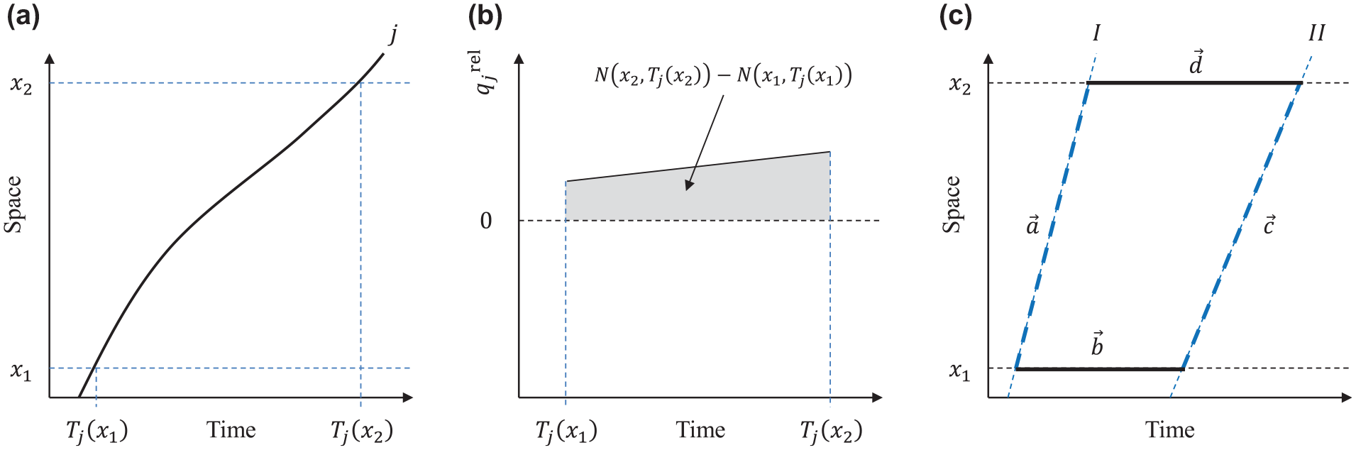
The position of vehicle $j$ at time $t$ is described by $X_{j} (t)$ . Furthermore, the probe vehicle speed can be obtained by taking the derivative to time of the probe vehicle position, that is, $V_{j} (t) = \partial_{t} X_{j} (t)$ . Figure 1a shows the trajectory, that is, position over time, of probe vehicle $j$ .

Figure 1.

Visualizations related to the theoretical foundations. (a) Probe trajectory $X_{j} (t)$ , (b) probe relative flow and change in cumulative flow, and (c) area enclosed by two observation paths of stationary observers and two probe trajectories.

The cumulative flow $N$ along the probe trajectory is given by $N (X_{j} (t), t)$ , which we will denote as $N_{j} (t)$ . In multi-lane traffic, where overtaking is possible, $N_{j} (t)$ can change over time. The rate at which the cumulative flow along a probe trajectory changes over time is denoted as the probe relative flow and described by $q_{j}^{rel} (t) = \partial_{t} N_{j} (t)$ . This probe-specific relative flow can be described as a function of the probe speed $V_{j} (t)$ and the macroscopic variables, that is:

q_{j}^{rel} (t) = k (X_{j} (t), t) [u (X_{j} (t), t) - V_{j} (t)]

(1)

A positive value indicates that $N_{j}$ increases over time, which means that probe $j$ is overtaken by more vehicles than it overtakes; that is, it is a relatively slow vehicle.

The change in cumulative flow $Δ N$ along the probe trajectory between two locations ( $x_{1}$ and $x_{2}$ ) can be described as a function of the relative flow. For this purpose, we take the integral of the probe relative flow between the period that is considered:

N (x_{2}, T_{j} (x_{2})) - N (x_{1}, T_{j} (x_{1})) = \int_{T_{j} (x_{1})}^{T_{j} (x_{2})} q_{j}^{rel} (t)

(2)

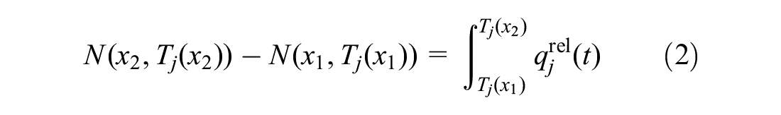
where $T_{j} (x_{1})$ and $T_{j} (x_{2})$ respectively denote the times at which probe $j$ passes locations $x_{1}$ and $x_{2}$ .

Figure 1b visually shows how Equation 2 can be interpreted. The probe relative flow $q_{j}^{rel} (t)$ is indicated by the solid black line. The area under this line describes the change in cumulative flow over the probe trajectory between $x_{1}$ and $x_{2}$ , that is, $N (x_{2}, T_{j} (x_{2})) - N (x_{1}, T_{j} (x_{1}))$ .

Equations 1 and 2 state that the change in cumulative flow along a probe trajectory depends on the probe speed and the macroscopic variables along this trajectory. In this study, probe trajectory data are considered that do not contain observations of the relative flow. However, the relations provided in this section show that other data related to the macroscopic variables (i.e., detector data) can be used to estimate the probe relative flow. Therefore, in the next section, a methodology is proposed to estimate the change cumulative flow along probe trajectories using detector data.

Differences in the Change in Cumulative Flow between Probe Trajectories

Equation 2 shows that it is possible to evaluate the accuracy of $q_{j}^{rel} (t)$ -estimates if the cumulative flow curves at $x_{1}$ and $x_{2}$ are known, that is, if we know $N (x_{1}, T_{j} (x_{1}))$ and $N (x_{1}, T_{j} (x_{1}))$ . However, as explained in the introduction, real detector data alone do not provide accurate information on these curves as they need to be initialized and we need to mitigate the cumulative error problem. Below, we propose an approach to evaluate the $Δ N$ -estimates along two (consecutive) probe trajectories based on detector data. This approach does not require initialization of cumulative flow curves and is less sensitive to the cumulative error problem as it only uses the detector passings in a short time period.

Let us consider a combination of two (consecutive) detectors and two (consecutive) probe vehicles; see Figure 1c. The thick solid black lines in this figure show the observation paths of the detectors, and the thick dashed blue lines show two probe trajectories. In case we combine detector and probe trajectory data, the change in cumulative flow $Δ N$ is observed over the black lines ( $\vec{b}$ and $\vec{d}$ ), but not over the blue lines ( $\vec{a}$ and $\vec{c}$ ). Conservation-of-vehicles determines that the net flow over the enclosed area boundary needs to be equal to zero:

Δ N_{\vec{b}} + Δ N_{\vec{c}} = Δ N_{\vec{a}} + Δ N_{\vec{d}}

(3)

where the elements in the left part ( $Δ N_{\vec{b}}$ and $Δ N_{\vec{c}}$ ) and the right part ( $Δ N_{\vec{a}}$ and $Δ N_{\vec{d}}$ ) of the equation are, respectively, positive when there is an inflow into or outflow out of the area. The individual changes in cumulative flow are given by:

Δ N_{\vec{a}} = N (x_{2}, T_{I} (x_{2})) - N (x_{1}, T_{I} (x_{1}))

(4)

Δ N_{\vec{b}} = N (x_{1}, T_{II} (x_{1})) - N (x_{1}, T_{I} (x_{1}))

(5)

Δ N_{\vec{c}} = N (x_{2}, T_{II} (x_{2})) - N (x_{1}, T_{II} (x_{1}))

(6)

Δ N_{\vec{d}} = N (x_{2}, T_{II} (x_{2})) - N (x_{2}, T_{I} (x_{2}))

(7)

In Equation 3, $Δ N_{\vec{a}}$ and $Δ N_{\vec{c}}$ describe the changes in cumulative flows over the probe trajectories, which in turn depend on the probe relative flows, see Equations 1 and 2:

Δ N_{\vec{a}} = \int_{T_{I} (x_{1})}^{T_{I} (x_{2})} q_{I}^{rel} (t)

(8)

Δ N_{\vec{c}} = \int_{T_{II} (x_{1})}^{T_{II} (x_{2})} q_{II}^{rel} (t)

(9)

The other parts of Equation 3, that is, $Δ N_{\vec{b}}$ and $Δ N_{\vec{d}}$ , describe the true changes in cumulative flow over detectors. In case of observation errors $ε$ , the observed changes in cumulative flow $Δ \hat{N}$ can differ from the true changes in cumulative flow $Δ N$ , that is:

Δ N_{\vec{b}} = Δ {\hat{N}}_{\vec{b}} + ε_{\vec{b}}

(10)

Δ N_{\vec{d}} = Δ {\hat{N}}_{\vec{d}} + ε_{\vec{d}}

(11)

Therefore, we can describe the sum of the (net) detector observation errors ( $ε_{\vec{b}}$ and $ε_{\vec{d}}$ ) and (net) change in cumulative flow over probe trajectories ( $Δ N_{\vec{a}}$ and $Δ N_{\vec{c}}$ ) based on the observed changes in cumulative flow ( $Δ {\hat{N}}_{\vec{b}}$ and $Δ {\hat{N}}_{\vec{d}}$ ):

Δ {\hat{N}}_{\vec{d}} - Δ {\hat{N}}_{\vec{b}} = Δ N_{\vec{c}} - Δ N_{\vec{a}} + ε_{\vec{b}} - ε_{\vec{d}}

(12)

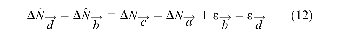
This relation is used in the empirical case study to evaluate the accuracy of estimates related to the change in cumulative flow along probe trajectories (i.e., $Δ N_{\vec{a}}$ and $Δ N_{\vec{c}}$ ). The left side of this equation is observed using detectors, whereas $Δ N_{\vec{a}}$ and $Δ N_{\vec{c}}$ are estimated. By comparing $Δ {\hat{N}}_{\vec{d}} - Δ {\hat{N}}_{\vec{b}}$ and the estimates of $Δ N_{\vec{c}} - Δ N_{\vec{a}}$ , we gain insight in the combination of observation and estimation errors.

Methodology to Estimate the Change in Cumulative Flow between Detectors

To estimate the change in cumulative flow over probe trajectories between detectors, we will rely on disaggregated detector data. Disaggregated lane-specific detector data are collected using double loop-detectors. These data describe each individual passing $n$ of detector $d$ in lane $l$ . This passing is described by the passing time $T_{l}^{d} (n)$ and passing speed $V_{l}^{d} (n)$ .

The disaggregated data can be used to calculate the macroscopic traffic states. Within a defined period $p$ with duration $Δ t$ , the flow and mean speed are respectively calculated by dividing the number of passing by the period duration and by taking the harmonic mean speed of the individual speeds related to the relevant passings. This yields $q (x_{d}, p)$ and $u (x_{d}, p)$ where $x_{d}$ denotes the location of detector $d$ . In line with Edie’s generalized definitions of traffic flow, the harmonic mean speed is taken instead of the arithmetic mean speed. Based on the flow and mean speed, we calculate the density, that is, $k (x_{d}, p) = q (x_{d}, p) / u (x_{d}, p)$ .

Equation 1 shows how the probe relative flow relates to the macroscopic traffic-flow variables and the individual probe speed. This equation is applied to estimate the probe relative flow at the times that it passes the detector locations. For this purpose, a time-window of length $Δ t$ around the time at which the probe passes detector $d$ is selected; that is, the detector passings between $t = T_{j} (x_{d}) - Δ t / 2$ and $t = T_{j} (x_{d}) + Δ t / 2$ are used to estimate the macroscopic variables.

The detector data provide probe relative flow $q_{j}^{rel} (t)$ estimates for the times at which the probe passes the upstream and downstream detector locations $x_{1}$ and $x_{2}$ , that is, $T_{j} (x_{1}))$ and $T_{j} (x_{2}))$ . However, to estimate the change in cumulative flow between $x_{1}$ and $x_{2}$ , we need estimates for the full period between $T_{j} (x_{1})$ and $T_{j} (x_{2})$ .

Depending on probe vehicle driving behavior and the traffic conditions that are encountered by the probe vehicle, the probe relative flow can change along its trajectory. The probe trajectory data contain information on the probe speed $V_{j} (t)$ along the full probe trajectory. Changes in the probe speed indicate that the relative flow has changed; however, a decrease in probe speed does not mean that the relative flow has to increase. A relatively fast probe may reduce its speed because it encounters congestion, but may (still) be a relatively fast vehicle. Furthermore, in congested conditions the density is higher than in free-flow conditions. This means that, following Equation 1, the probe relative flow may even decrease when the probe speed decreases, as a result of decreasing mean speed and increasing density.

As the probe speed does not provide sufficient information to estimate $q_{j}^{rel} (t)$ , we solely rely on the estimates of $q_{j}^{rel} (T_{j} (x_{1}))$ and $q_{j}^{rel} (T_{j} (x_{2}))$ to estimate the probe relative flow along the full trajectory. For this purpose, we consider a simple scheme in which the probe-specific relative flow linearly changes between detector locations:

q_{j}^{rel} (t) = ϕ (t) q_{j}^{rel} (T_{j} (x_{1})) + (1 - ϕ (t)) q_{j}^{rel} (T_{j} (x_{2}))

(13)

where $x_{1}$ and $x_{2}$ denote the upstream and downstream detector locations and the weight factor $ϕ (t)$ is given by:

ϕ (t) = \frac{T_{j} (x_{2}) - t}{T_{j} (x_{2}) - T_{j} (x_{1})}

(14)

If we solely want to estimate the change in cumulative flow along the probe vehicle between the detector locations, that is, $N (x_{2}, T_{j} (x_{2})) - N (x_{1}, T_{j} (x_{1}))$ , Equations 13 and 14 simplify to:

\begin{matrix} N (x_{2}, T_{j} (x_{2})) - N (x_{1}, T_{j} (x_{1})) \\ = \frac{q_{j}^{rel} (T_{j} (x_{1})) + q_{j}^{rel} (T_{j} (x_{2}))}{2} [T_{j} (x_{2}) - T_{j} (x_{1})] \end{matrix}

(15)

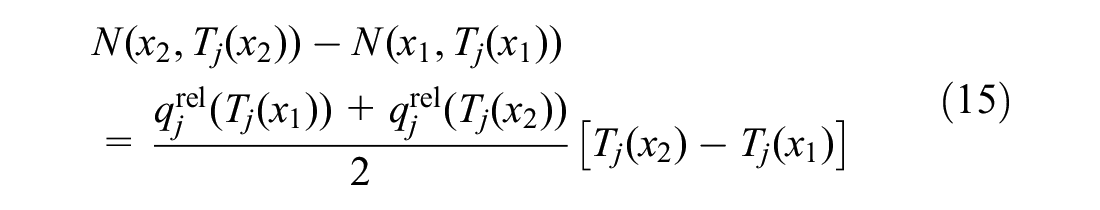
In this study, we consider this simple (linear) scheme to estimate how the probe-specific relative flow changes between detector locations. This scheme solely uses probe data that describe the times and speeds at which the probe passes the detectors and detector data around these times. If the traffic conditions change significantly along the probe trajectory, this scheme may be too simplistic. In our experiment, we will evaluate the effect of the traffic condition on the accuracy of this scheme. Furthermore, it is important to note that more extensive schemes may be used that incorporate information related to the full probe trajectory and potentially also estimates of the traffic state between the detectors. The former would require that we have high-frequency probe data, whereas for the considered scheme it suffices that probe vehicle share the time and speed at which they pass the detector locations. For the latter (i.e., estimating the traffic state between detectors), different methodologies to estimate the traffic state may be used, for example, the ASM-filter ( 19 ).

Case Study

In the case study, both real and simulated traffic data are used. Real data have the advantage of real traffic behavior and real observation errors. However, we lack a ground truth for real data. Therefore, we also use microscopic simulation to construct traffic-sensing data with similar characteristics, while having access to a ground truth.

Below, we first explain which traffic-sensing data are collected for the two studies and which traffic conditions occur in the study period and road stretch. Next, we explain which experiments will be conducted and which insights these experiments should provide.

Traffic-Sensing Data and Traffic Conditions

Figure 2 shows the road layouts and traffic conditions for the two case studies. For both studies, we will discuss which data are available and why certain study periods are selected.

Figure 2.

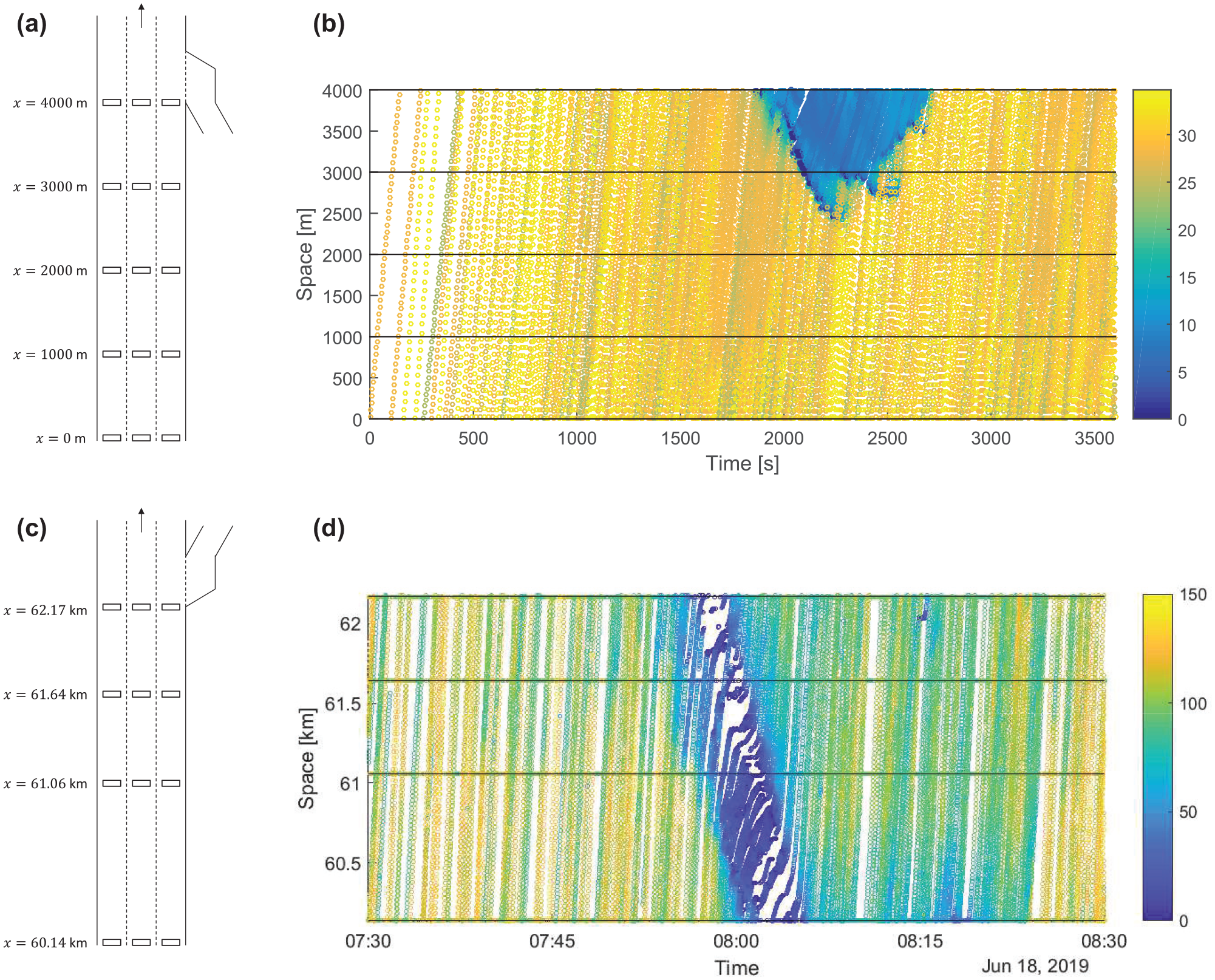
Road layouts and traffic conditions for the two case studies. (a) Road layout, simulation study, (b) individual vehicle speeds (m/s) (every 10th vehicle), simulation study, (c) road layout, empirical study, and (d) individual probe vehicle and detector passing speeds (km/h), empirical study.

Simulation Study

In the simulation study, the microscopic simulation program FOSIM ( 18 ) is used. The model used in this program is validated for Dutch freeway traffic ( 20 ). Figure 2a shows that we consider a three-lane road segment with an on-ramp that is located at $x = 4000$ m. In the simulation, the on-ramp traffic causes congestion that spills back on the link upstream of the on-ramp, see Figure 2b. Detectors are located at $x = 0, 1000, 2000, 3000, 4000$ m, which provide disaggregated detector data.

Empirical Study

Real disaggregated detector and probe trajectory data are available for a test section on the A9 in The Netherlands on June 18th, 2019. These data are respectively made available by the Dutch road authority (RWS) and BeMobile as part of a project that aims to evaluate the value of fusing these two data types to gain more accurate traffic state estimates and potentially reduce the required road-side sensing equipment. BeMobile provides high-frequency (1 s) probe GPS-data, which are map-matched by Modelit. This yields probe trajectory data that describe the position over time (i.e., trajectory) of a subset of the vehicles (i.e., the probe vehicles).

The layout (including detectors locations) of the road segment that is considered in the empirical study is shown in Figure 2c. An off-ramp is located directly downstream of the considered segment. Two 1-hour peak-periods are selected, that is, 07:30–08:30 h and 16:00–17:00 h. These periods are selected to study the effect of changing traffic conditions on the ability to correctly estimate the change in cumulative flow over probe trajectories between detector locations. In the first period, some probes experience congested conditions, see Figure 2d. This figure shows that a stop-and-go wave propagates upstream. The cause of this jam lies downstream of the considered segment. In the second period, solely free-flow conditions are observed.

Experimental Set-Up

Multiple experiments are performed that provide insight in the estimation accuracy. The aim of the experiments is to evaluate the accuracy of estimating the change in cumulative flow over probe trajectories between two detector locations based on disaggregated detector data.

Selecting the period is a trade-off between capturing the local and current traffic conditions (which may be missed if we consider a very long period) and observing extreme flow values (which may happen if we consider a very short period). We tested with periods of 30 s, 60 s, and 120 s. Although small changes are observed in the results, the overall findings and conclusions remain the same. Therefore, we solely present the estimates resulting from using $Δ t = 60$ s, which aligns with the standard aggregation period of detector data in The Netherlands.

In both the empirical and simulation studies, we compare the estimates for different detector spacings. In the simulation study, the considered detector spacings are 1,000, 2,000, 3,000, and 4,000 m. In the empirical study, the considered detector spacings are 920, 1,500, and 2,030 m (which includes all detectors installed on the test section).

The availability of the ground truth in the simulation study allows us to visualize and quantify the estimation errors. As this provides a detailed insight into the estimation performance, we will first perform the simulation study. The resulting insights help to analyze the results of the empirical study.

In the simulation study, two steps are taken. First, we compare the estimated and true changes in cumulative flow ( $Δ N$ ) for all vehicles. For this purpose, a scatter plot is constructed with the estimated and true $Δ N$ , respectively, on x-axis and y-axis. Furthermore, the vehicle travel time is indicated by the color of the dots. In these figures, two $Δ N$ errors can be distinguished: 1) The error if it is assumed that the cumulative flow does not change along the probe trajectory—as assumed in other studies ( 9 , 14 , 16 )—is indicated by the vertical distance between the dots and the true change in cumulative flow is zero. For this purpose, a horizontal dashed black line is drawn for ‘true $Δ N = 0$ ’. 2) The error that remains after correction-based detector data is indicated by the horizontal/vertical difference between the dots and the diagonal black line. These errors are also represented using the error statistic Root Mean Squared Error (RMSE), where we make a difference between vehicles that experience congestion between detectors and those that do not. Second, to gain a deeper understanding of the underlying factors that influence the estimation accuracy, the estimates related to four individual vehicles are studied in more detail. For these vehicles, time-series plots are constructed of the true and estimated changes in cumulative flow, and the vehicle speed.

Because of the absence of the ground truth, it is not possible to directly compare the estimated and true changes in cumulative flow over probe trajectories for the empirical study. Therefore, an alternative comparison is considered in the empirical study; we analyze the difference in $Δ N$ , that is, the difference in the net number of (-) overtakings, between two consecutive probe vehicles. As explained in the section “Theoretical foundations,” this difference can be observed using detector data. The observed difference can be compared with the probe-specific relative flow estimates. In line with the simulation study, we construct a scatter plot the shows the estimated (x-axis) and observed (y-axis) difference in $Δ N$ between two consecutive probe vehicles. As the observations relate to two probes, the color of the dots is based on the mean travel time. The ability to explain the difference in $N$ based on the detector data is indicated by the differences between the dots on the black diagonal line. It is important to note that the observed difference is still subject to detector count errors; see Equation 12. Detectors may miss or double count passing vehicles. A lane change might cause a vehicle to miss a detector, but perhaps also two detectors in adjacent lanes can both be triggered ( 21 ). However, evaluation of the empirical data indicates that the number of missed or double-counted vehicles is limited. Comparing the cumulative number of passings of consecutive detectors shows that the difference only slowly increases. This means that there is a need to address the cumulative error problem (in which the presented methodology can be used), but that the effect of these errors on the methodology and evaluation of it is very limited.

Results

This section presents the results from the simulation study and the empirical study. The simulation study is discussed first because it yields insights that are valuable in analysis the empirical study results.

Simulation Study

Figure 3 shows the true and estimated change in cumulative flow over vehicle trajectories between two detector locations. In these figures the vehicle travel time between detectors is indicated by the color. Furthermore, Figure 4 shows time-series of the true and estimated change in cumulative flow together with the individual speed for four vehicles. These time-series are used to provide more detailed explanations on the features that are observed in Figure 3.

Figure 3.

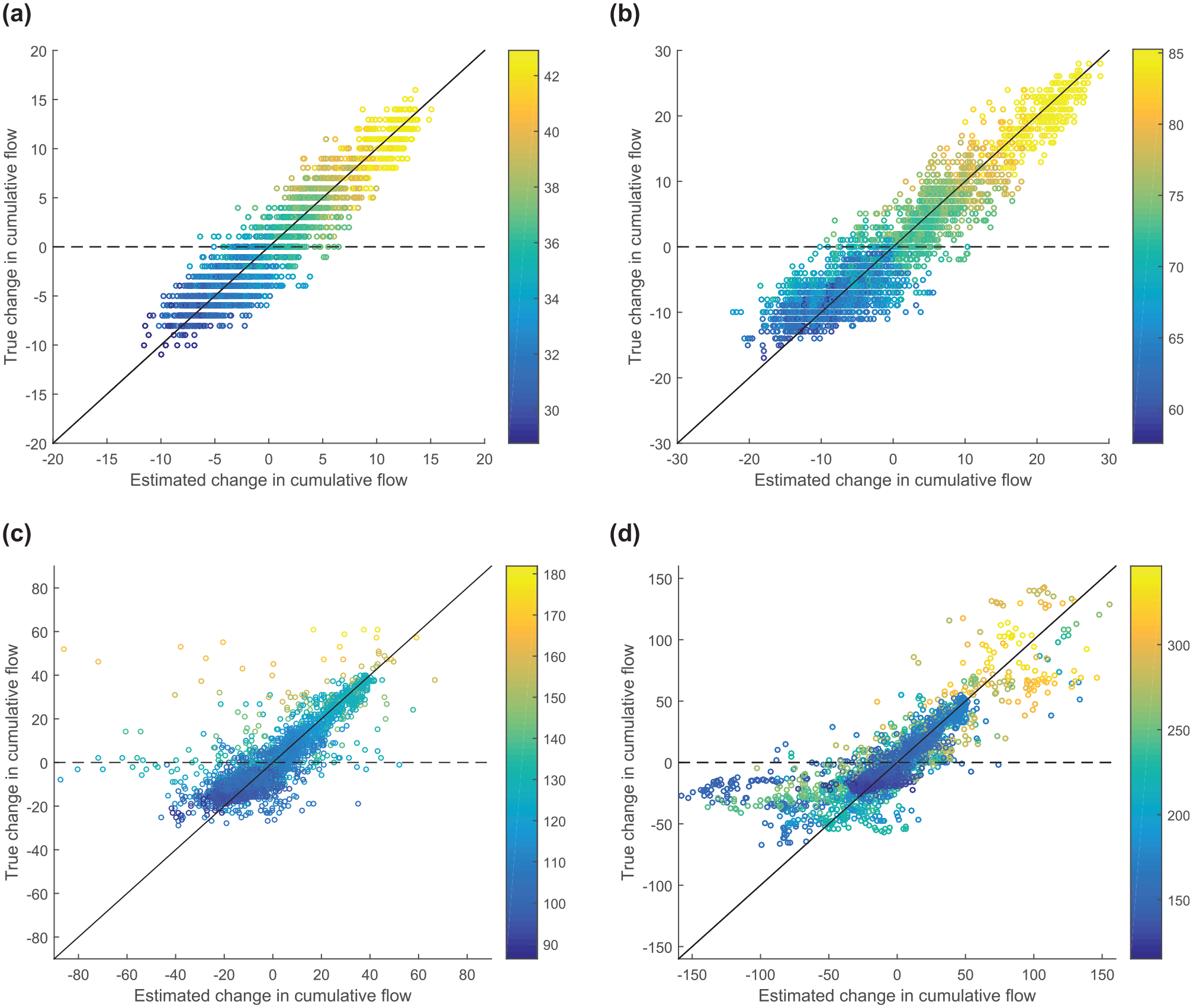
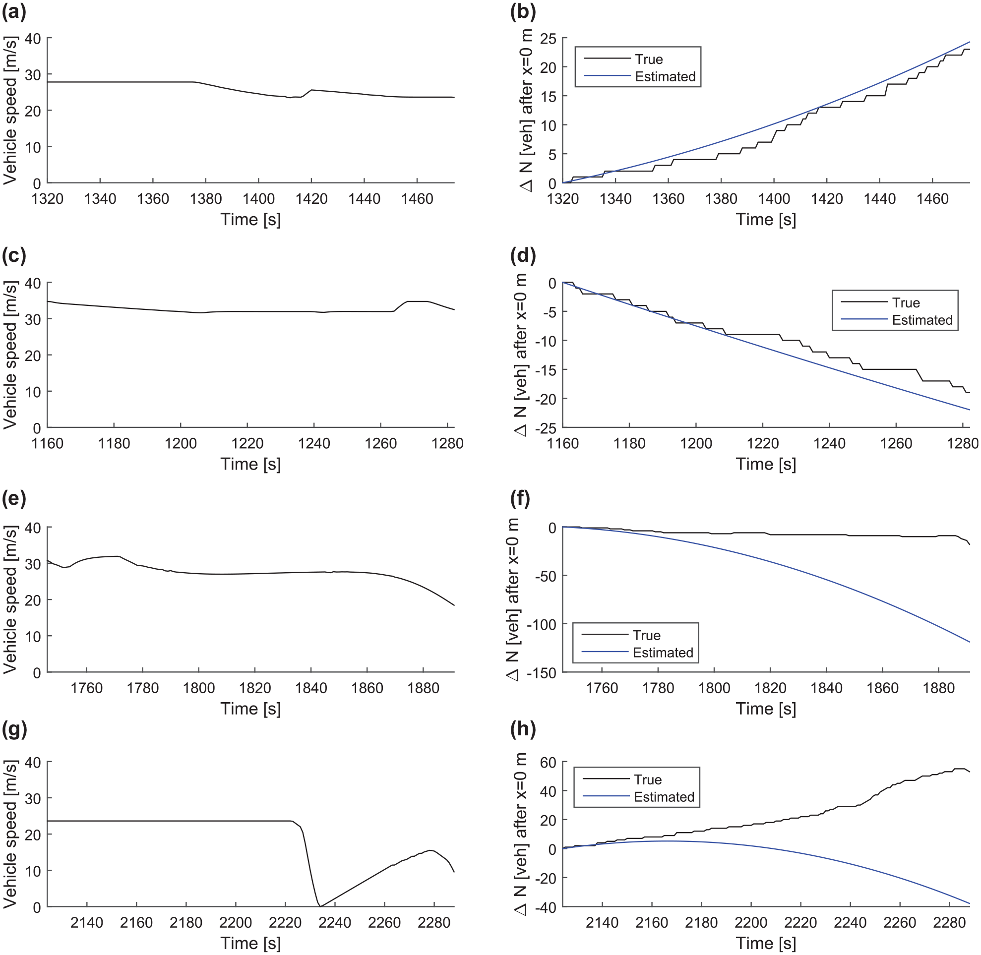
Simulation study: True and estimated change in cumulative flow over vehicle trajectories between two detector locations. The color of the dots indicates the vehicle travel time between the considered detector locations. (a) Between detectors located at $x = 0$ m and $x = 1000$ m (solely free-flow conditions), (b) between detectors located at $x = 0$ m and $x = 2000$ m (solely free-flow conditions), (c) between detectors located at $x = 0$ m and $x = 3000$ m (free-flow and congested conditions), and (d) between detectors located at $x = 0$ m and $x = 4000$ m (free-flow and congested conditions).

Figure 4.

Simulation study: True and estimated changes in the cumulative flow over probe trajectories together with the probe speeds. (a) Slow vehicle solely in free-flow, (b) slow vehicle solely in free-flow, (c) fast vehicle solely in free-flow, (d) fast vehicle solely in free-flow, (e) fast vehicle shortly experiencing congestion at downstream detector, (f) fast vehicle shortly experiencing congestion at downstream detector, (g) slow vehicle shortly experiencing negative relative flow, and (h) slow vehicle shortly experiencing negative relative flow.

In free-flow conditions, estimating the change in cumulative flow over vehicle trajectories is a clear improvement over assuming that there is no overtaking. As the congestion does not spill back upstream of $x = 2500$ m, Figure 3, a and b , solely include vehicle trajectories in free-flow conditions. These figures show that the solid black line is a better fit than the dashed black line, which indicates that estimation is an improvement over assuming “no overtaking.” This is also indicated by an improvement in the RMSE, that is, it improves from 5.11 vehicles to 1.65 vehicles for the detector spacing of 1,000 m, and from 9.25 vehicles to 3.18 vehicles for the detector spacing of 2,000 m, see Table 1. Figure 4, a–d , show the vehicle speed and lane together with the estimated and true change in cumulative flow between $x = 0$ m and $x = 4000$ m for a relatively slow and fast vehicle that solely travel in free-flow conditions. These figures show that the change in cumulative flow is estimated relatively accurate along the vehicle trajectory.

Table 1.

Error Statistics for the Four Detector Spacings.

Detector spacing (m)	Travel time threshold (s)	Correction using detector data		Assume no overtaking
Detector spacing (m)	Travel time threshold (s)	RMSE FF (vehicles)	RMSE CG (vehicles)	RMSE FF (vehicles)	RMSE CG (vehicles)
1,000	45	1.65	na	5.11	na
2,000	90	3.18	na	9.25	na
3,000	135	7.92	29.55	13.29	30.58
4,000	180	17.85	28.51	18.16	44.02

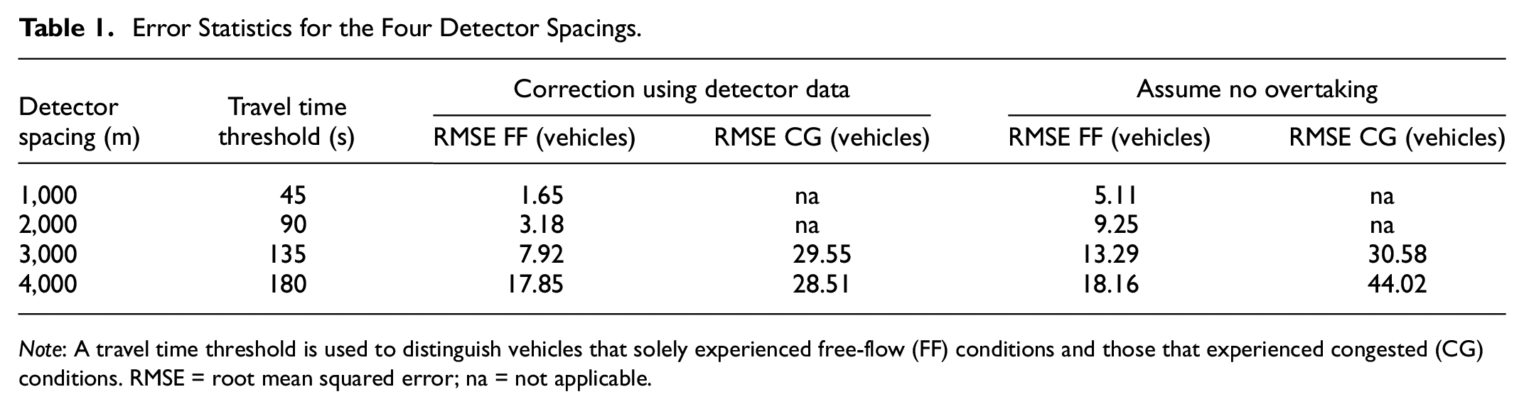
Note: A travel time threshold is used to distinguish vehicles that solely experienced free-flow (FF) conditions and those that experienced congested (CG) conditions. RMSE = root mean squared error; na = not applicable.

If vehicles experience congested conditions, the estimated changes in cumulative flow are less accurate than for vehicle solely experiencing free-flow conditions, that is, the black diagonal line is a better fit for Figure 3, a and b , than for Figure 3, c and d ; however, also in these cases it is still more accurate to estimate the change in cumulative flow than assume “no overtaking,” see Table 1. In this table for a detector spacing of 4,000 m, the RMSE of vehicles solely experiencing free-flow conditions is relatively large with respect to the other spacings, that is, it jumps from 7.92 vehicles to 17.85 vehicles for detector spacings of 3,000 m and 4,000 m, respectively. In Figure 3d there are some observations that show a travel time below the threshold (i.e., smaller than 180 s) and for which the change in cumulative flow is highly underestimated (i.e., estimates around $Δ N = - 125$ vehicles, while the true $Δ N$ are approximately −25 vehicles). Let us look at Figure 4, e and f , to study this in more detail. Figure 4f shows that $Δ N$ is highly underestimated for this vehicle. It also shows that the true $Δ N$ reduces sharply in the last second that the vehicle is between the detectors and Figure 4e shows that at the same time the vehicle speed decreases. At this last period, the vehicle experiences congested conditions, but is relatively fast, which results in a short highly negative relative flow. In this case the relative flow observed at the downstream detector is not representative of the full trajectory, which causes a large error in the estimated change in cumulative flow. The large underestimation of $Δ N$ in Figure 3c (large negative estimates, while the true values are positive) can be explained using the same principle; see Figure 4, g and h . In these figures, we show a vehicle between $x = 0$ m and $x = 3000$ m for the estimated $Δ N$ is negative because of a large negative vehicle relative flow at the downstream detector.

Empirical Study

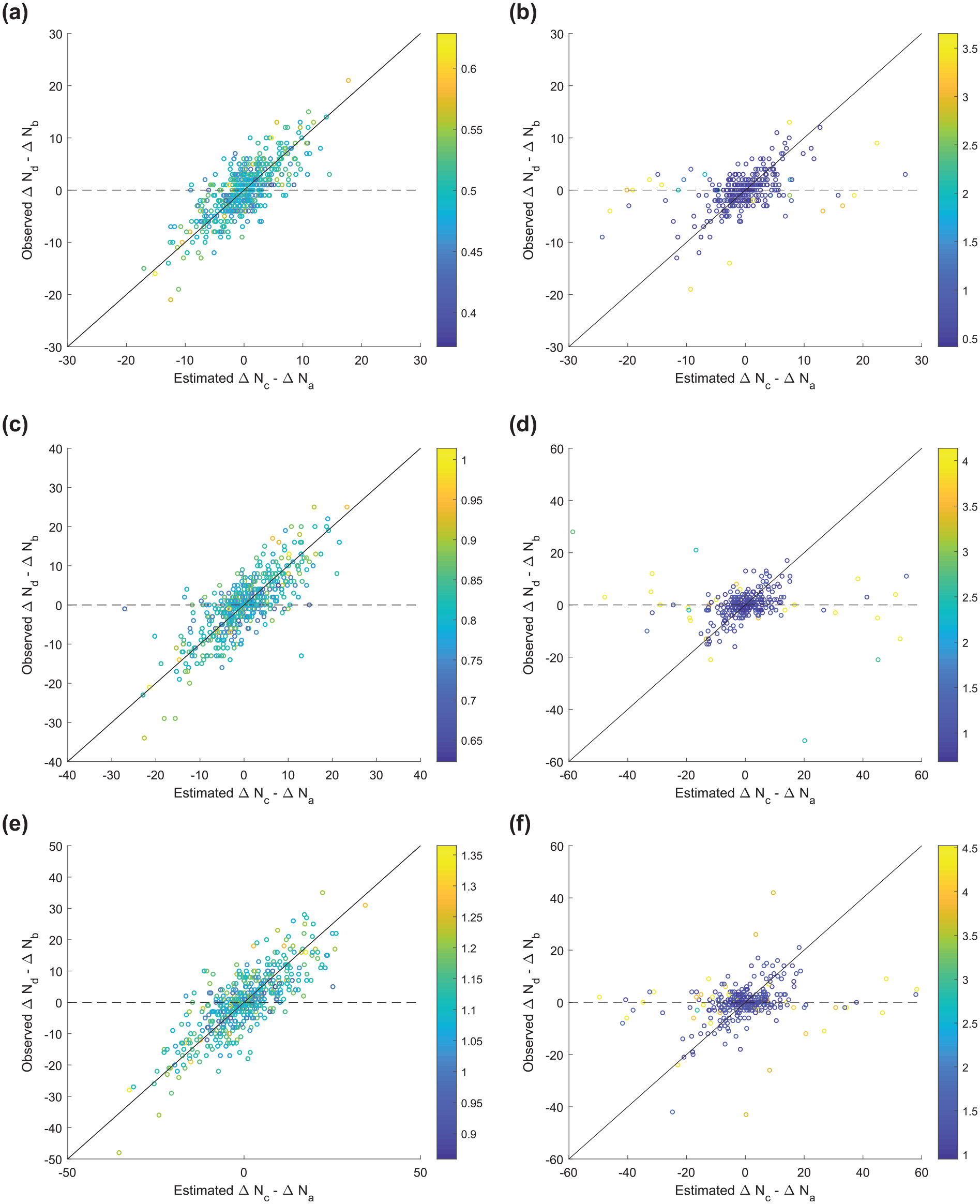
Figure 5 shows the results of the empirical case study. The axes are the same for all subfigures, that is, Estimated $Δ N_{\vec{c}} - Δ N_{\vec{a}}$ (x-axis) and Observed $Δ N_{\vec{d}} - Δ N_{\vec{b}}$ (y-axis). The section “Theoretical foundations” explains the details behind comparing these two features. In short, both axes relate to the difference in the number of vehicles that overtake two consecutive probes between the detector locations. The y-axis describes this feature based on the detector passing observations, whereas the x-axis shows the result of the estimated change in cumulative flow along the two probe trajectories.

Figure 5.

Empirical study: The difference in the number of vehicles that overtake two consecutive probes between the detector locations based on detector passing observations (y-axis) and probe relative flow estimates (x-axis). The color of the dots indicates the mean travel time between the considered detector locations of the two consecutive probes. (a) Between detectors at $x = 60.14$ km and $x = 61.06$ km, free-flow period, (b) between detectors at $x = 60.14$ km and $x = 61.06$ km, period with congestion, (c) between detectors at $x = 60.14$ km and $x = 61.64$ km, free-flow period, (d) between detectors at $x = 60.14$ km and $x = 61.64$ km, period with congestion, (e) between detectors at $x = 60.14$ km and $x = 62.17$ km, free-flow period, and (f) between detectors at $x = 60.14$ km and $x = 62.17$ km, period with congestion.

In line with the simulation study, the empirical results indicate that estimation of the change in cumulative flow between detectors is relatively accurate in free-flow conditions, see Figure 5, a , c and e . Also here, the estimates are better than assuming that $Δ N = 0$ , thus the points are better aligned with the diagonal line. To get an insight in the potential mean error of assuming “no overtaking” during the considered period, we may look at the mean estimated change in cumulative flow along individual trajectories between detectors. For the three detector spacings, that is, 920, 1,500 and 2,030 m, these mean $Δ N$ are, respectively, equal to 3.26, 5.45 and 7.49 vehicles.

In congestion, the computed relative flow is not very accurate in estimating the real number of vehicles passed; see Figure 5, b , d and f . These figures do not show a good relation between the two axes. The largest differences are observed for probes that have a high mean travel time, which means that these probes are affected by the stop-and-go wave. The figures indicate that the probe relative flows estimated at the detectors are not representative for the full probe trajectory between detectors. The simulation study also showed that the estimation performance decreased when probes experience congestion; however, the estimation performance in congestion for the simulation study seems to be better than for the empirical study. This can partially be explained by the different features that we compare. Figure 5 uses the estimates related to two probes. If these errors have the same sign (+ or –), the total absolute error increases, which leads to large positive or negative values of $Δ N_{\vec{c}} - Δ N_{\vec{a}}$ . Another potential reason for the low estimation performance lies in the lane-drop directly upstream of the first detector (which is used in all estimates). The stop-and-go wave that propagates upstream in the considered period causes a standing queue at this lane-drop. Figure 2d show that the vehicles passing the detector at $x = 60.14$ km are affected by this queue (which is indicated by the lower speeds at the upstream detector between 08:00 h and 08:45 h). This effect can result in probe relative flow estimates that are not representative for the full probe trajectory, and thereby cause errors in the $Δ N$ -estimates.

Conclusion and Insights

Probe trajectory or vehicle re-identification data can be used for initialization and error correction of cumulative flow curves constructed using stationary detectors. Studies that use these data for this purpose often assume that there is no overtaking, which would mean that the cumulative flow value is constant along a probe trajectory. However, in multi-lane traffic, this assumption is often violated. This study investigates the option to estimate the change in cumulative flow along probe trajectories based on disaggregated detector data, and in this way improve on the “no overtaking” assumption.

In this study, both simulated as real data are used to investigate the changes in cumulative flow along probe trajectories and the ability to expose this using detector data. By means of a case study we show that the probe relative flow estimated at two detector locations is representative for the full trajectory between these locations in free-flow conditions. Therefore, in these conditions it is a clear improvement to describe the change in cumulative flow based on detector data instead of assuming “no overtaking.” If probe vehicles experience congestion between detectors, the probe relative flows estimated at the detector locations are less representative for the rest of the trajectory. In the simulation study (where the estimation accuracy can be quantified), using disaggregated detector data still yields more accurate estimates than assuming “no overtaking.” However, in the empirical study, these benefits are not observed. Changing traffic conditions along the probe trajectory (which are related to ability to estimate the change in cumulative flow based on detector data) can be observed using the probe speed. This means that the probe speeds observed between detectors could and should be used to assign an uncertainty to the estimates of the change in cumulative flow along probe trajectories.

More complex schemes may be used that may include information such as the probe speed and the traffic states along the trajectory between detector locations. Probe trajectory data provide information on the probe speeds between detector locations; however, the data do not contain exact information on the traffic state between these locations. Estimating the traffic states between detector locations is the intended application and is the reason for estimating the relative flows along probe trajectories. The circular relation between estimating the probe-specific relative flows and estimating the traffic state indicates that an (iterative) optimization approach to estimate both features is potentially interesting. However, in this study, we focused on the first step and evaluate how accurate the probe-specific relative flows can be estimated without estimating the macroscopic traffic states along the full probe trajectory.

Footnotes

Acknowledgements

We would to extend our appreciation for all parties that provided the funding and data for this study.

Author Contributions

P. B. C. van Erp has taken the lead in conceptualizing the idea, data analysis and writing the article, V. L. Knoop has provided regular feedback during all phases of the project, E. Smits was involved in the data analysis and provided feedback on the manuscript, C. Tampère has been involved in conceptualizing the idea, and S. P. Hoogendoorn provided feedback during all phases of the project.

Declaration of Conflicting Interests

The author(s) declared no potential conflicts of interest with respect to the research, authorship, and/or publication of this article.

Funding

The author(s) disclosed receipt of the following financial support for the research, authorship, and/or publication of this article: This study was funded by the Netherlands Organization for Scientific Research (NWO), grant-number: 022.005.030. The data used in this study were provided by the Dutch road authority Rijkswaterstaat, BeMobile and Modelit.

References

Seo

Bayen

A. M.

Kusakabe

Asakura

Traffic State Estimation On Highway: A Comprehensive Survey. Annual Reviews in Control, Vol. 43, 2017, pp. 128–151.

Papageorgiou

Hadj-Salem

Blosseville

ALINEA: A Local Feedback Control Law for On-Ramp Metering: A Real-Life Study. Transportation Research Record: Journal of the Transportation Research Board, Vol. 1320, 1991, pp. 58–64.

Hoogendoorn

S. P.

Landman

Van Kooten

Schreuder

Integrated Network Management Amsterdam: Control Approach and Test Results. Proc., 16th International IEEE Conference on Intelligent Transportation Systems (ITSC 2013), pp. 474–479.

Makigami

Newell

G. F.

Rothery

Three-Dimensional Representation of Traffic Flow. Transportation Science, Vol. 5, No. 3, 1971, pp. 302–313.

Newell

G. F.

A Simplified Theory of Kinematic Waves in Highway Traffic, Part I: General Theory. Transportation Research Part B: Methodological, Vol. 27, No. 4, 1993, pp. 281–287.

Laval

J. A.

Castrillon

Stochastic Extension of Newells Three-Detector Method. Transportation Research Record: Journal of the Transportation Research Board, Vol. 2315, 2012, pp. 73–80.

Claudel

C. G.

Bayen

A. M.

Lax-Hopf Based Incorporation of Internal Boundary Conditions into Hamilton-Jacobi Equation. Part I: Theory. IEEE Transactions on Automatic Control, Vol. 55, No. 5, 2010, pp. 1142–1157.

Claudel

C. G.

Bayen

A. M.

Lax-Hopf Based Incorporation of Internal Boundary Conditions into Hamilton-Jacobi Equation. Part II: Computational Methods. IEEE Transactions on Automatic Control, Vol. 55, No. 5, 2010, pp. 1158–1174.

Sun

Jin

W. L.

Ritchie

S. G.

Simultaneous Estimation of States and Parameters in Newell’s Simplified Kinematic Wave Model with Eulerian and Lagrangian Traffic Data. Transportation Research Part B: Methodological, Vol. 104, 2017, pp. 106–122.

10.

Van Erp

P. B. C.

Knoop

V. L.

Hoogendoorn

S. P.

On the Value of Relative Flow Data. Transportation Research Part C: Emerging Technologies, Vol. 13, 2020, pp. 74–90.

11.

Daganzo

C. F.

A Variational Formulation of Kinematic Waves: Basic Theory and Complex Boundary Conditions. Transportation Research Part B: Methodological, Vol. 39, No. 2, 2005, pp. 187–196.

12.

Daganzo

C. F.

A Variational Formulation of Kinematic Waves: Solution Methods. Transportation Research Part B: Methodological, Vol. 39, No. 10, 2005, pp. 934–950.

13.

Van Erp

P. B. C.

Knoop

V. L.

Hoogendoorn

S. P.

Macroscopic Traffic State Estimation using Relative Flows from Stationary and Moving Observers. Transportation Research Part B: Methodological, Vol. 114, 2018, pp. 281–299.

14.

Van Lint

J. W. C.

Hoogendoorn

S. P.

A Generic Methodology to Estimate Vehicle Accumulation on Urban Arterials by Fusing Vehicle Counts and Travel Times. Presented at 94th Annual Meeting of the Transportation Research Board, Washington, D.C., 2015.

15.

Van Erp

P. B. C.

Knoop

V. L.

Hoogendoorn

S. P.

Estimating the Vehicle Accumulation: Data-Fusion of Loop-Detector Flow and Floating Car Speed Data. Presented at 97th Annual Meeting of the Transportation Research Board, Washington, D.C., 2018.

16.

Bhaskar

Chung

Dumont

A. G.

Fusing Loop Detector and Probe Vehicle Data to Estimate Travel Time Statistics on Signalized Urban Networks. Computer-Aided Civil and Infrastructure Engineering, Vol. 26, No. 6, 2010, pp. 433–450.

17.

Takenouchi

Kawai

Kuwahara

Traffic State Estimation and Its Sensitivity Utilizing Measurements From the Opposite Lane. Transportation Research Part C, Vol. 104, 2019, pp. 95–109.

18.

Dijker

Knoppers

FOSIM 5.1 Gebruikershandleiding (Users Manual). Technical Report, Technische Universiteit Delft, 2006.

19.

Treiber

Helbing

Reconstructing the Spatio-Temporal Traffic Dynamics from Stationary Detector Data. Cooper@tive Tr@nsport@tion Dyn@mics, Vol. 1, 2002, pp. 3.1–3.24.

20.

Henkens

Mieras

Bonnema

Validatie FOSIM. Technical Report, Sweco, De Bilt, 2017.

21.

Knoop

V. L.

Wilson

R. E.

Buisson

van Arem

Number of Lane Changes Determined by Splashover Effects in Loop Detector Counts. IEEE Transactions on Intelligent Transportation Systems, Vol. 13, No. 4, 2012, pp. 1525–1534.

Estimation of the Change in Cumulative Flow over Probe Trajectories using Detector Data

Abstract

Theoretical Foundations

Change in Cumulative Flow along a Probe Trajectory

Differences in the Change in Cumulative Flow between Probe Trajectories

Methodology to Estimate the Change in Cumulative Flow between Detectors

Case Study

Traffic-Sensing Data and Traffic Conditions

Simulation Study

Empirical Study

Experimental Set-Up

Results

Simulation Study

Empirical Study

Conclusion and Insights

Footnotes

Acknowledgements

Author Contributions

Declaration of Conflicting Interests

Funding

References