
Abstract
Lane drops are a common bottleneck source on motorway networks. Congestion sets in upstream of a lane drop as a result of the lane changing activity of merging vehicles. This causes the queue discharge rate at the bottleneck to decrease and drop below the capacity, leading to capacity drop and further congestion. The objective of this study is to minimize the total travel time of the system by controlling lateral flows upstream of the lane drop. This is equivalent to maximizing the exit flows at the bottleneck. An optimization problem is formulated for a 3–2 lane drop section with high inflow. The problem is solved for different test cases where the direction of lateral flows being controlled is varied. An incentive based macroscopic model representing the natural lane changing scenario is used as a benchmark for comparison. The results showed that by influencing the lateral flows upstream of the bottleneck, the queue discharge rate increased by more than 4.5%. The total travel time of the system was consequently found to be reduced. The improvements in performance were primarily a result of the distribution of lane changing activity over space and the balancing of flow among the lanes which lead to the decrease in the severity of congestion. The findings reveal a potentially effective way to reduce the severity of congestion upstream of lane drop bottlenecks during high demand which could be implemented using roadside and in-car advisory systems.
Traffic jams on motorways are becoming a common phenomenon across the world. Lane drops are a common source of bottlenecks on motorways. Lane drops are locations where the number of lanes provided for through traffic decreases. These areas are prone to congestion because traffic in the lane dropping has to merge into the through lane and the high lane changing (LC) activity results in congestion. When congestion sets in upstream of a lane drop bottleneck, the discharge flow rate drops below the capacity of the bottleneck which is known as capacity drop. Capacity drop upstream of lane drops (or merging sections) has been observed in multiple studies ( 1 , 2 ). Sub-optimal LC and high demand can trigger congestion at the lane drops and the capacity of the bottleneck drops when it is most required. With the emergence of technologies such as vehicle-to-infrastructure (V2I) and advanced driver-assistance systems (ADAS), it is possible to develop active traffic management strategies which can improve the traffic flow at these bottlenecks and avoid, delay, or at least reduce the level of congestion and accidents. Depending on the conditions, the proportions of flows in different lanes vary on multilane motorways ( 3 , 4 ). Unbalanced lane usage can lead to a reduction in the capacity of the motorways. By using these emerging technologies and developing appropriate lateral control strategies, balanced lane usage can be obtained which can improve the overall throughput at such bottleneck locations.
There have been multiple studies on traffic control at lane drop bottlenecks. These control measures include: (a) the use of variable speed limits (VSL); (b) lane assignment; (c) integrating VSL with LC control or ramp metering (at merging sections); (d) microscopic control; and others which were tested using traffic flow models. We will now discuss the literature on these elements.
VSL is a well-known and studied control strategy which is used to smooth traffic flows and regulate inflow ( 5 , 6 ). Jin and Jin evaluated the effect of VSL in a zone upstream of a lane drop bottleneck ( 7 ). The study found that VSL strategies based on integral (I) and proportional integral (PI) controllers could effectively mitigate congestion and reduce the travel time when capacity drop occurred but could not improve the performance of the traffic system without a capacity drop. Carlson et al. developed feedback based VSL controllers for lane drop bottlenecks and tested these strategies via METANET which is a second-order macroscopic traffic flow model ( 8 , 9 ). Roncoli et al. proposed a feedback control strategy for lane assignment at lane drops using a first-order macroscopic multilane traffic flow model proposed in ( 10 ) which also accounted for the capacity drop phenomenon ( 11 ). Results showed that the control strategy was able to improve the traffic performance. Zhang et al. proposed a lane-changing advisory control in the merge lane of a lane drop to distribute LC using Cooperative Intelligent Transport Systems (C-ITS) technology ( 12 ). Improvements in the traffic flow efficiency and a reduction in the total travel time (TTT) was observed as a result of the LC advisories. Zhang et al. developed a combined LC and VSL control strategy that recommended LCs in advance to relieve capacity drop for truck dominated highways ( 13 ). LC commands were given as advice to the drivers and were defined according to a set of case-specific rules. Similar studies integrating VSL with other traffic control measures such as ramp metering have been developed and simulated for merging bottlenecks such as ( 14 – 17 ). There are other studies microscopic in nature where the longitudinal motions of individual vehicles were controlled to create gaps near merging locations and to facilitate the LC process ( 18 – 22 ).
Most of the existing studies focus on VSL or a combination of VSL and LC control measures to improve the traffic performance. Sub-optimal LCs are one of the primary reasons for the occurrence of capacity drop at lane drop bottlenecks and LC control can be used for efficient traffic management at such locations. In Zhang et al., only the LCs from the leftmost lane were analyzed and the lane changing in other lanes was not taken into consideration ( 12 ). While Zhang et al. considered a combination of VSL and LC control, the LC strategies were based on case-specific rules and therefore might not be optimal ( 13 ). In Roncoli et al., the LC flows which were controlled were not constrained by the capacity of the receiving lanes and were rather bound by a threshold value and LC flows were considered in only one direction ( 11 ). LC control in combination with other control measures has been studied ( 11 , 13 , 23 ) but in general, there is further potential to exploit lateral interventions to improve traffic performance.
This study provides a framework for determining ideal lateral flows upstream of a lane drop during high demand to improve the traffic flow efficiency. This will provide a foundation for developing effective traffic management strategies using in-car and roadside systems for such locations. As the traffic stream is considered macroscopically, the implementation of developed control measures to model individual vehicle movements according to the identified LC strategy is out of the scope of this study.
The remainder of the paper is organized as follows: the next section introduces the incentive based first-order multilane traffic flow model which is used as the base case representing the natural LC scenario. The section following this presents the network used in this study and the description of the base case. This is followed by the section describing the optimization problem formulation and the different cases that will be compared with the base case. In the results section, solutions of the optimization and discussions on the performance of the different control cases are provided. Finally, the paper concludes with recommendations for future work.
Incentive Based Multilane First-Order Traffic Flow Model
To test and compare the performance of the proposed strategy, an incentive based first-order traffic flow model is used. The authors refer to Nagalur Subraveti et al. for a complete description of the model (
24
). For self-containedness, a brief description is provided here. A multilane motorway subdivided into segments, where each segment comprises several lanes is shown in Figure 1. The segments are indexed
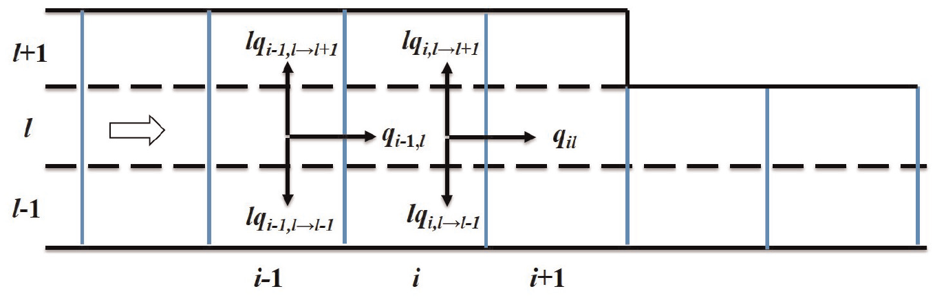
Representation of the discretized motorway.
Using the notations from Figure 1, the conservation equation in discrete terms is given by:
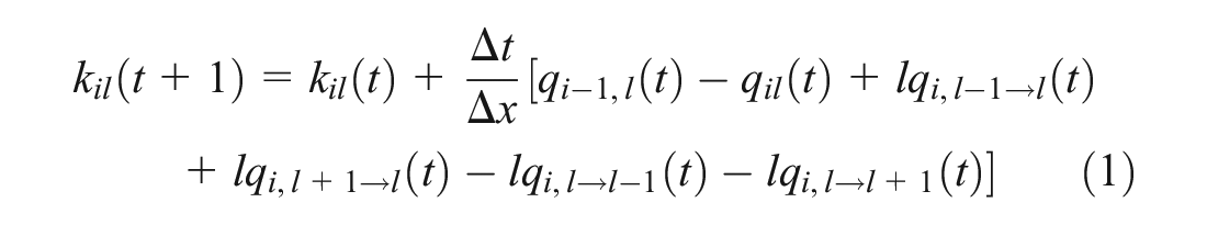
where
To ensure numerical stability based on the Courant-Friedrichs-Lewy (CFL) condition ( 25 ), the cell length must obey the following condition:

where

The triangular fundamental diagram (FD) is used for computing the lateral and longitudinal flows.
Computation of Lateral Flows
The fraction of flow with a desire to change lanes is computed as a function of the density difference among lanes (

The incentives are designed for smaller cell segment sizes and may not work well when the cell segments are too long (in the order of 1 km). To consider the effect of downstream conditions, a weighted density term is considered which is the weighted average of the density of the considered cell segment and its two downstream cell segments in the same lane with weights of 2, 2, and 1 respectively. The fraction of flow with a desire to change lane from

where
Computation of Longitudinal Flows
The longitudinal flow transferred from an upstream cell

The longitudinal flow is given as the minimum of demand

where

The supply of cell

where

The actual LC flow
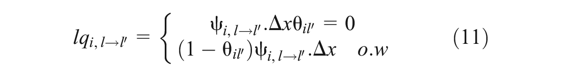
To incorporate the capacity drop phenomenon in the first-order model, the supply function of the receiving cell is modified where the receiving capacity of the downstream cell
The model was tested against real world data for a lane drop section on a motorway in the Netherlands. It was observed that the model was able to capture the relevant lane level dynamics in relation to the lane flow distribution and merging activity near the lane drop with an error of 2–3 vehicles per kilometer per lane in relation to estimating lane-specific densities. The model was also compared with a linear regression model and the results showed that this model performed much better than the regression model. Therefore, it can be said with reasonable confidence that the model represents reality and is therefore used for the base case to represent the LC activity near lane drops.
Network Description and Base Case
A hypothetical motorway stretch is considered to evaluate the performance of the proposed strategy. The schematic of the lane drop used in the study is shown in Figure 2a. The network consists of a three-lane motorway with a left lane drop from three to two lanes after 3.3 km. The section upstream of the bottleneck is labeled as A–B while the downstream section is referred to as B–C.
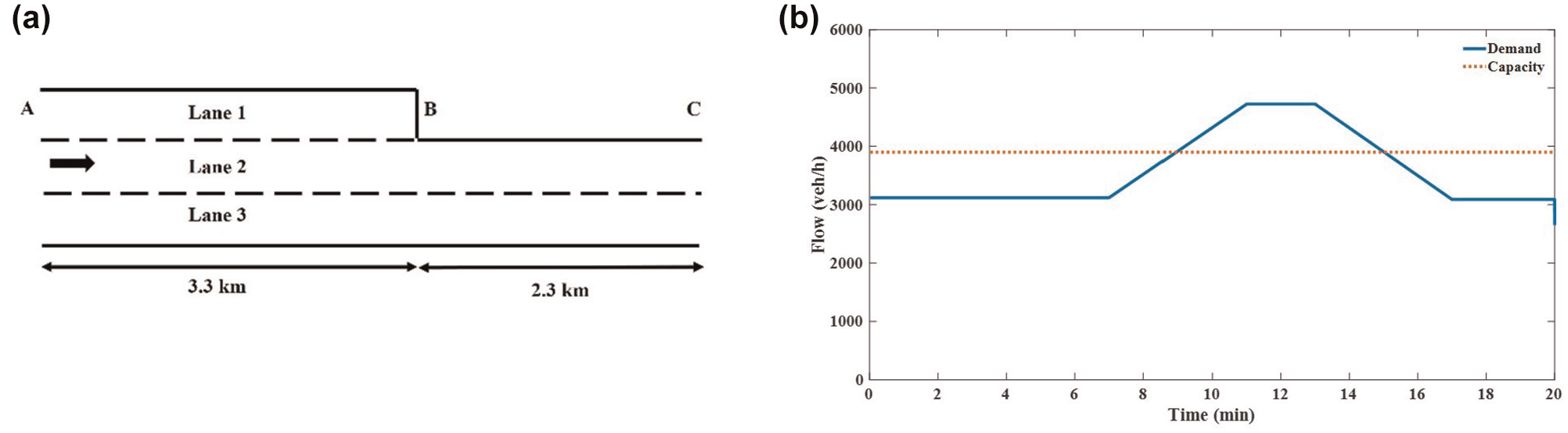
Simulation setup: (a) benchmark network layout; and (b) demand profile used for simulations.
The lane-specific FD parameters used in the incentive based traffic model are given in Table 1.
Lane-Specific FD Parameters
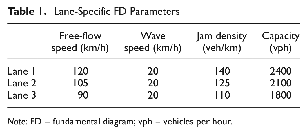
Note: FD = fundamental diagram; vph = vehicles per hour.
The simulation time step is chosen to be 1s. The total simulation time is 30 min. Lateral flows are controlled at every 1 min. The demand profile considered for the simulation study is shown in Figure 2b. The demand is constant for the first 7 min followed by a gradual rise. This increase in demand leads to the onset of congestion upstream of the bottleneck. The demand is at its peak value for a period of 2 min. The demand then gradually decreases until it is lower than the capacity of bottleneck and remains constant at this value till the end of the 20th minute. The flow entering the section is stopped after 20 min and the simulation is run for another 10 min to allow all the vehicles to exit the section. The demand in the individual lanes is always maintained lower than or equal to their capacities. The framework was also tested for two other different demand profiles where the duration of peak demand as well as the slope of the rise in demand to peak values were varied.
The chosen FD parameters result in a critical density of 20 veh/km in each lane. Considering a triangular FD, any density above the critical density implies that the lane is in a state of congestion. The chosen time step and FD parameters will result in a cell length of (120/3.6) m upstream of the lane drop and (105/3.6) m downstream of the lane drop via Equation 3. This amounts to a total of 180 cells in each lane of the network (100 upstream and 80 downstream of the lane drop).
Optimization Problem Formulation
This section presents the framework of the optimization problem aimed at determining the ideal lateral flows upstream of a 3–2 lane drop bottleneck to improve the traffic flow efficiency. The objective function chosen for the optimization problem and the numerical implementation are initially discussed followed by a description of the two test cases of the optimization problem. This is followed by a section describing the decision variable chosen for the optimization problem to influence the lateral flows.
Objective Function and Optimization Approach
The optimization algorithm attempts to find lateral flows which can minimize the TTT of the system. When the initial cell segments in a section get congested, the flow that can enter at a particular time step will be less than the actual demand because of the reduced capacity of the receiving cell. While this can lead to reduced TTT within the section, this can cause the vehicles to queue at the entrance of the section leading to a high TTT outside the section. Thus, to include the delay as a result of the queue formation at the entrance of the section, an additional term representing the time spent by vehicles queuing at the entrance of the mainline is included in the TTT computation. Thus, the objective function is given as:
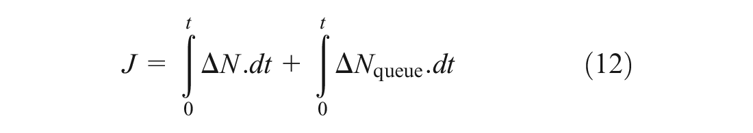
where
The first term of the objective function represents the TTT within the network and the second term represents the time after a vehicle would like to enter the network and before it can actually enter the network. The origins are modeled with a vertical queue model where the net demand (

The numerical algorithm used to solve the optimization problem is the MATLAB implementation of the Sequential Quadratic Programming (SQP) algorithm (fmincon). The algorithm requires an initial guess as an input. In this case, the lateral flows obtained from the base case are used as the initial solution guess. The optimization framework is also tested for different initial solutions to get a feeling for the variations in any capacity gains observed.
Unilateral and Bilateral Case
Two different cases are considered for the optimization problem: the unilateral case; and the bilateral case. The optimizer tries to find suitable lateral flows which can minimize the TTT of the system. In the unilateral case, lateral flows are influenced in only one direction that is, from left to right. LCs are prohibited from right to left in this case. Therefore, LCs can occur from lanes 1 and 2 to lanes 2 and 3 respectively while no lane changing is allowed from lanes 3 and 2 to lanes 2 and 1 respectively.
In the bilateral case, LCs are influenced in both directions. The only exception to this is LC from lane 2 to lane 1. LC activity from 2 to 1 is generally too low because of the approaching drop in lane 1 and therefore for simplicity, lateral flows from lane 2 to lane 1 are assumed to be zero. The only difference between the unilateral and bilateral case is therefore that LCs are allowed from lane 3 to lane 2 in the bilateral case. A net lateral flow term is considered between lanes 2 and 3 in the bilateral case. This ensures that the lateral flow is moving in only one direction at a particular location. There is a possibility that LCs are suggested in both directions at the same locations. To avoid the problem of lane hopping, a single lateral flow term is therefore considered. The net lateral flow between lanes 2 and 3 is given by:

If
Decision Variable
The variable manipulated to minimize the designed objective function is the fraction of flow wanting to change lane
The lateral flows are influenced upstream of the lane drop bottleneck. There are 100 cell segments in each lane upstream of the bottleneck which will result in 200 (300) decision variables in the unilateral (bilateral) case. Computation of
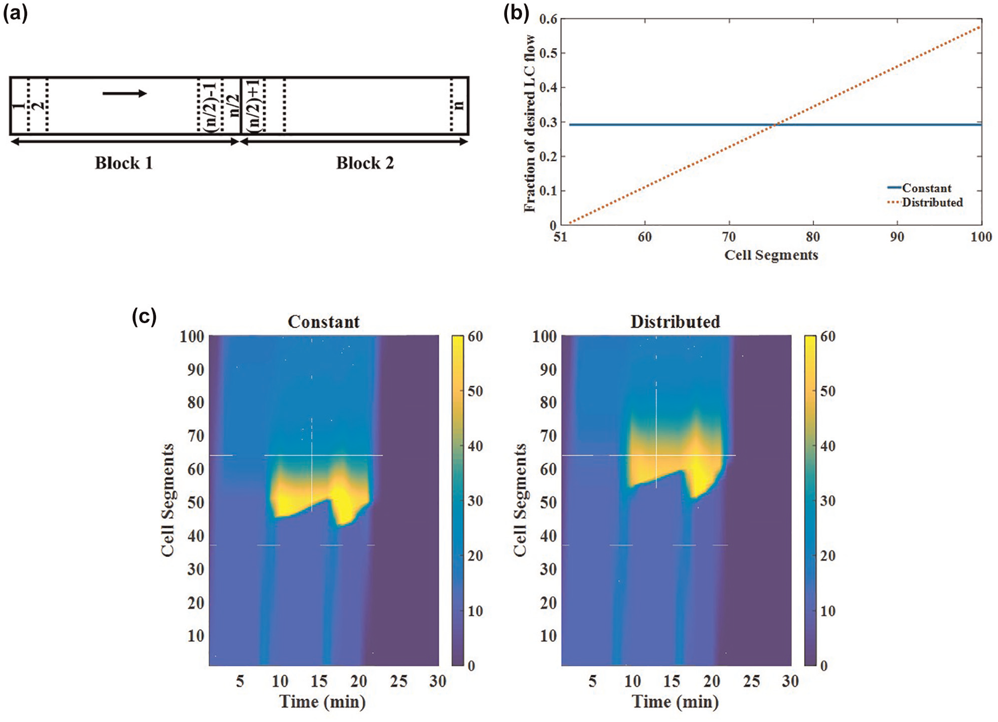
Difference between cell segments and blocks: (a) schematic of a block containing cell segments; (b) distribution of the fraction of desired lane changing (LC) flow among cell segments in a block; and (c) density contour plots (veh/km) of lane 2 for different LC rates of cell segments in a block.
The decision variables in the unilateral case are:

In the bilateral case, the decision variables are:

The value of
If we assume a constant value of
Results
This section presents the results of the base case and compares it with the two other test cases discussed in the previous section. The results of the base case are obtained by using the incentive based traffic flow model. The TTT is compared for the three cases followed by discussions on the optimal solution and reasons for improvement in the test cases. Only the results for the demand profile described in the previous section are discussed in detail as similar patterns are observed for all the scenarios.
TTT Comparison
Table 2 shows the comparison of the three different cases in relation to the TTT of the system.
Comparison of TTT for the Different Cases
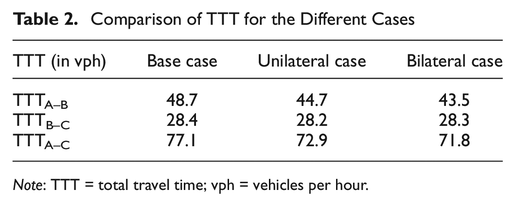
Note: TTT = total travel time; vph = vehicles per hour.
The base case where no LC strategy is implemented and the lateral flows are computed from the traffic flow model results in a TTT of 48.7 veh/h in the section A–B which is upstream of the bottleneck. Both unilateral and bilateral cases result in lower TTT for this section as compared with the base case. A decrease of 8.3% and 10.6% in the TTT are observed in the unilateral and bilateral cases respectively. As no LC strategy was implemented downstream of the lane drop in any of the cases, not much difference in TTT is observed for section B–C which is in free flow. Therefore, it can be seen that influencing the lateral flows among lanes can indeed lead to reduced travel times upstream of the lane drop bottleneck.
Density Contour Plots
Figure 4a shows the density contour plots of lanes 2 and 3 for the three cases. Congestion occurs in all three cases because the demand entering the section is greater than the bottleneck capacity. It can be seen that the level of congestion (especially in lane 2) is reduced in the bilateral and unilateral cases as compared with the base case. In all cases, congestion begins after approximately 10 min as a result of the rise in demand. It can also be seen that the congestion is more spread in lanes 2 and 3 in the other two cases when compared with the base case. While the congestion seems to be spread evenly across the section in the unilateral case (especially in lane 3), it is more centered in the first block (up to 1.67 km) in the bilateral case for lanes 2 and 3. The density in lane 3 in the bilateral case is comparatively low in the first 9 min compared with the other two cases.
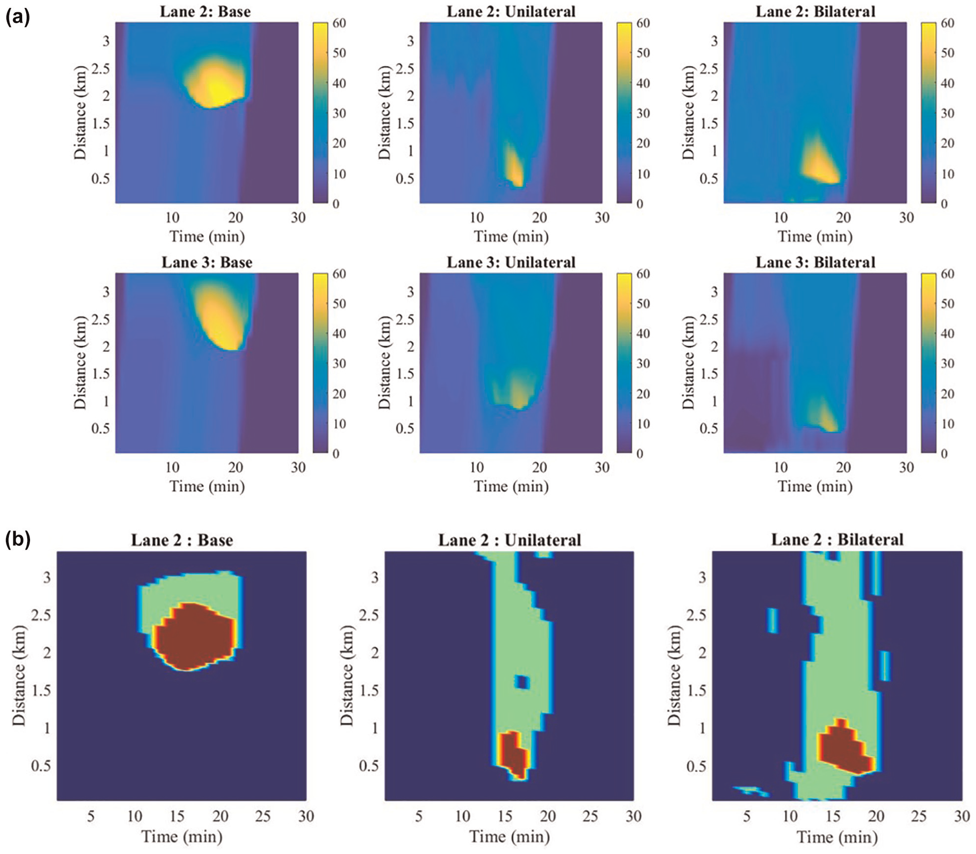
Comparison of traffic states for the different cases: (a) density (veh/km) plots for lanes 2 and 3; and (b) contour plot representing the ratio of the density of cell segment and critical density of cell segment for lane 2.
Figure 4b shows the plot for the ratio of density of cell segment and critical density of cell segment for lane 2 to check if the cells are indeed being fully used or if there is a further possibility to send lateral flows. The value of 0 on the color bar implies that the density of cells is lower than or equal to the critical density and, therefore, in free flow. A value of 1 implies that the density of the cells is greater than the critical density but lower than twice the critical density which are classified here as mildly congested. Cells where the ratio of density to critical density is greater than 2 are classified as severely congested. As can be seen from this figure, severe congestion for a long duration can be observed in the base case in lane 2 which is not seen in the test cases. Although there are regions of severe congestion in the unilateral and bilateral cases, they are spread over a small location and for a much shorter duration. The congested space is also spread out in the test cases while it is concentrated in the latter block in the base case. Similar patterns are observed in lane 3 where the cells are in mild congestion and the area of congestion is distributed throughout the section and regions of severe congestion are almost non-existent. It can also be inferred from this figure that the solution of lateral flows obtained from the optimization process is indeed close to optimal for reducing the travel times as any further increase of lateral flow from lane 1 can actually lead to severe congestion and a decrease in lateral flow can lead to under-utilization of lanes 2 and 3.
Optimal Solution: Lateral Flows and LC Strategy
In this section, the solutions obtained from the optimization process are discussed. The aim of the optimization process was to determine ideal lateral flows among lanes which can minimize the objective function described in Equation 12. Figure 5 shows the lateral flows across lanes for the different cases.
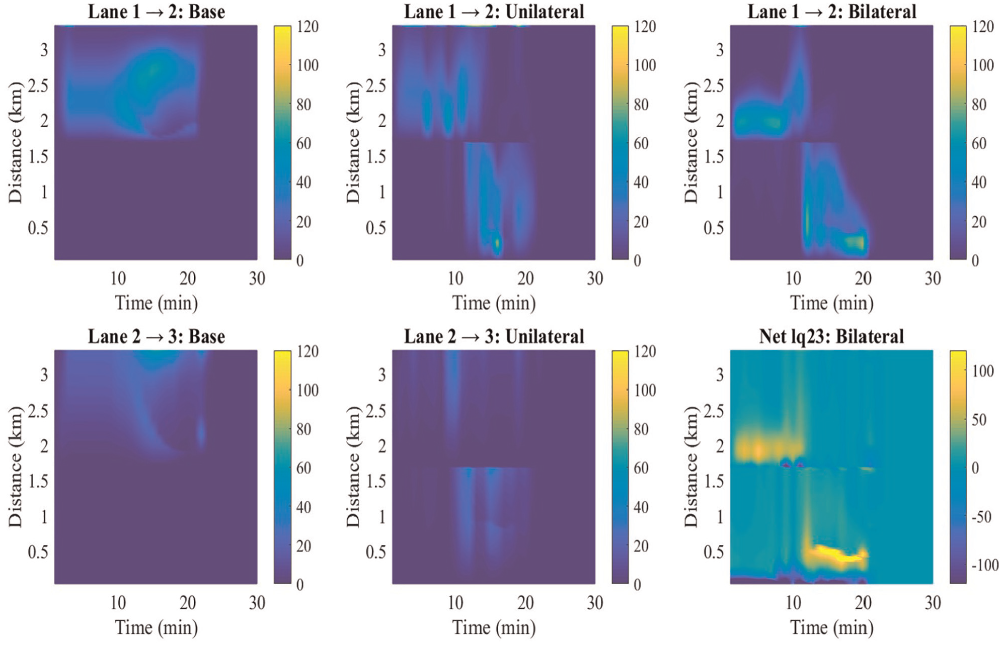
Lateral flow across lanes for the different control cases.
In the base case, the majority of the LC activity from lane 1 to 2 is observed in the final cell segments between 2 km and 3.3 km. Higher lateral flows can be observed between the 10th and 18th minute as a result of the increased demand which entered the section in the previous minutes. Some LCs occur from lane 2 to 3 to accommodate the incoming flow. This can be attributed to the combination of the density and cooperation incentives in the traffic flow model. As a result of the flow entering lane 2 from lane 1, the density of lane 2 increases which results in the activation of the density incentive leading to LCs from lane 2 to 3. The cooperation incentive in the model facilitates merging in lane 2 by allowing some LCs from lane 2 to 3 which is observed in reality. Negligible LC activity is observed from lane 3 to lane 2. The density in lane 2 is already high as a result of LCs from lane 1 and the keep-right incentive also restricts the number of LCs from lane 3. Compared with the base case, the lateral flows from lane 1 to 2 in both the unilateral and bilateral case are distributed over the entire space. It can be clearly observed that much more LCs occur in the first 50 segments between 0 and 1.67 km from lane 1 to 2 in both the test cases. The magnitude is a bit different in the two test cases. The “et_lq23” lateral flow plot of the bilateral case represents the net lateral flow between lanes 2 and 3 given by Equation 14. There is more flexibility in distributing the LC activity over space in the bilateral case as LCs are allowed in the other direction from lane 3 to lane 2. It can also be observed that the flow from lane 3 to 2 in the initial cells (0–0.5 km) in the bilateral case is high. This can be attributed to the higher prevailing speed in lane 2. As the objective of the optimization process was to minimize the TTT, LCs occur from lane 3 which has a lower free-flow speed to lane 2 which has higher free-flow speed. This is also the reason behind the low densities observed in lane 3 in the first 9 min in the bilateral case. This is not seen in the unilateral case as LCs from right to left are not allowed.
For the chosen demand profile, congestion is inevitable in the section. As the demand exceeds the bottleneck capacity, there is no way that congestion can be avoided. Capacity drop occurs in all three cases as a result of the onset of congestion upstream of the bottleneck. But the extent of reduction in the queue discharge rate differs in the three cases. Figure 6a shows the comparison between flow exiting the bottleneck. It can be seen that the queue discharge rate is clearly higher in the unilateral and bilateral case as compared with the base case. The queue discharge rate was found to be increased for all the demand profiles tested. The mean percentage increase in the queue discharge rate and the standard deviation compared with no control in the unilateral case were 4.8 and 0.5 respectively. Similarly, the mean percentage increase in the queue discharge rate and standard deviation for the bilateral case were 4.72 and 1.01 respectively. The sensitivity of the results to the value of the FD parameters was also analyzed by varying the lane-specific FD parameters. The individual FD parameters were varied within a ±5% range and the increase in queue discharge rate using the solution obtained from the optimization framework was observed for the unilateral case. Figure 6b shows the histogram of the percentage increase in queue discharge rate. It can be seen that in a majority of the cases, the increase in queue discharge rate is in the 4% to 5% range with a mean of 4.65 and a standard deviation of 1.4.
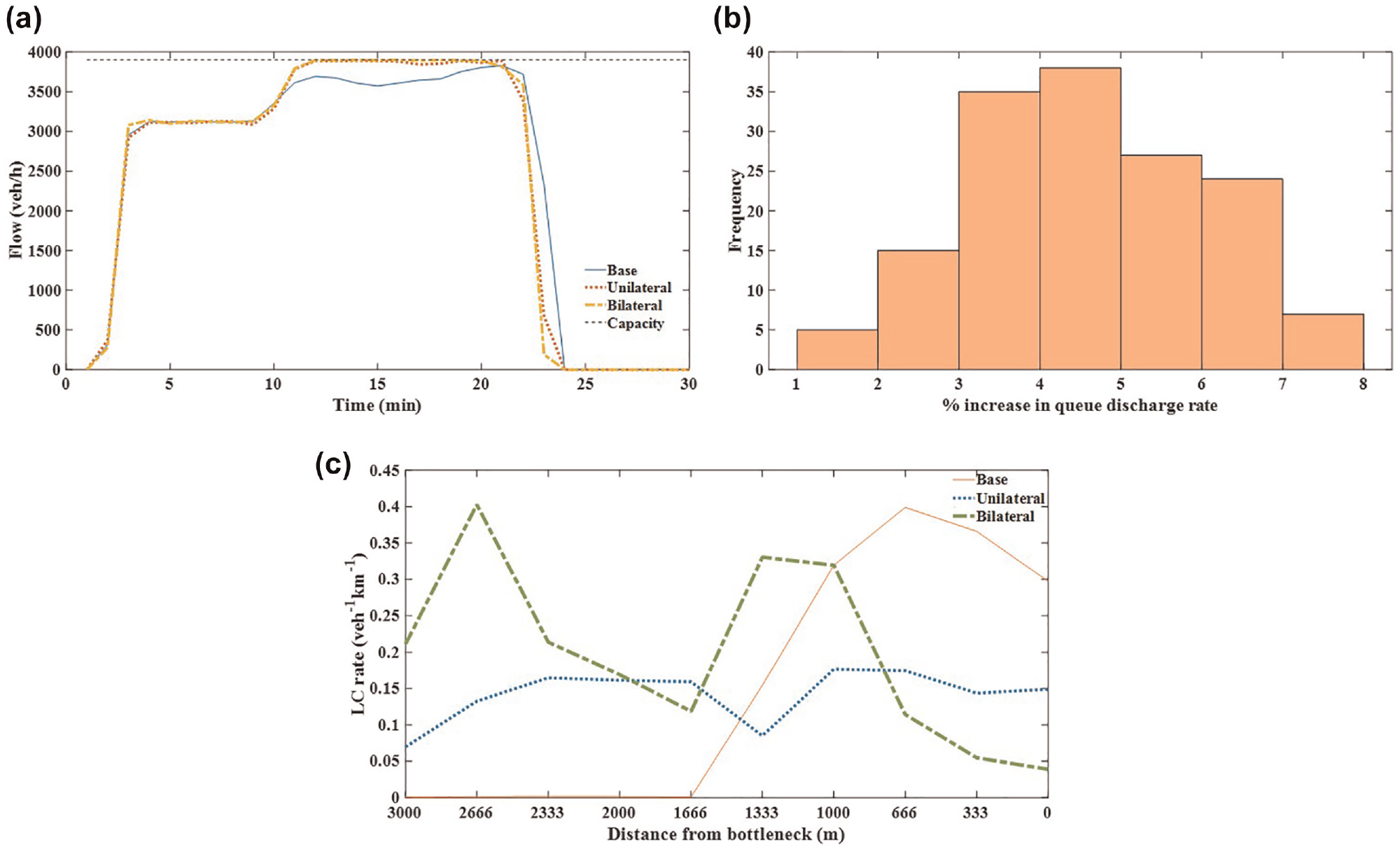
Simulation results: (a) flow exiting the bottleneck; (b) sensitivity of the results to fundamental diagram parameters; and (c) comparison of the lane changing rates upstream of the lane drop.
An alternate or simple case of avoiding congestion in the continuing lanes would be to control LCs from lane 1 in such a way that lanes 2 and 3 were always maintained at or below critical density. While this would ensure that the congestion did not form in lanes 2 and 3, heavy congestion would occur in lane 1 which would lead to high TTT and a possibility of congestion propagating backward in lane 1 and spilling to the adjacent lanes.
Figure 6c shows the comparison between the LC rates. In the base case, most of the LC activity occurs in the latter cells near the lane drop as seen from the rising LC rate. As a result of the continuous LCs from lane 1 at around the same location and rise in demand, congestion sets in. While there are some LCs from lane 2 to lane 3 to accommodate the incoming demand, they are not sufficient. In the other cases, the LC activity is more spread out.
The reduction in the severity of congestion and lower TTTs in the test cases occur for two reasons: distributing the LC activity over space instead of limiting it to locations just upstream of lane drop; and balancing the flows in each lane to accommodate the demands from the adjacent lanes. Similar findings were also revealed in ( 12 ) although they only considered LC from lane 1 to lane 2; LCs in other directions were not analyzed. Improvement in the performance of traffic flow cannot be achieved by either of these on their own. If the LC activity is distributed over the length of the section without a balancing of the flows, this would still cause congestion in lane 2 at the bottleneck. The pattern of congestion observed would be the same as in the test cases but with increasing severity of congestion as it nears the bottleneck. And by utilizing the space available in the adjacent lane via the balancing of flows without distributed LC activity, it would again lead to congestion similar to that observed in the base case with varying magnitude among lanes and reduced flow leaving the bottleneck. In the test cases, when LCs occur from lane 1 to lane 2 in one block, then LCs from lane 2 to lane 3 occur in the next block during the same time instant. This can be seen in Figure 5. In the base case, lane 3 is not utilized to its full extent. If we consider a 2–1 lane drop section, there is no extra lane available for the balancing of lateral flows and the only possibility is to spread out the LC activity. But this does not improve the efficiency of traffic flow. This reasoning has also been validated when the same demand profile, minus the demand in lane 3, was tested on a 2–1 lane drop section. No improvements in relation to reducing the TTT was found. Similarly, the benchmark network was tested for different demand profiles and similar patterns of lateral flows and improvements in queue discharge rate were observed. Thus, it can be inferred that in situations of high demand and LC activity upstream of a bottleneck, the severity of congestion and the extent of capacity drop can be reduced by distributing the LC activity and balancing the flows over lanes.
Conclusion
The main objective of this study was to identify LC strategies upstream of lane drop bottlenecks in case of high demand to reduce congestion as much as possible. To this end, an optimization problem was formulated in which the lateral flows were controlled on a 3–2 lane drop section. The objective of the optimization problem was to minimize the TTT of the section upstream of the lane drop bottleneck. The fraction of flow with a desire to change lanes is chosen as the decision variable as it directly relates to lateral flows and constraints can be fixed easily. Two different test cases were developed. In the first case, defined as unilateral, the lateral flows were regulated in only one direction (i.e., from left to right). The second case is termed bilateral where lateral flows are regulated in both directions. The test cases were compared with a base case which used an incentive based first-order traffic flow model. To reduce the size of solution space, lateral flows for an aggregation of cell segments called blocks were considered.
It was found that by influencing the lateral flows upstream of the lane drop, the queue discharge rate increased by more than 4.5% in both the test cases when compared with the base case for the various demand profiles. The TTT of the system was, therefore, also found to be reduced in the test cases. The analysis of the optimal solutions indicates that the improved performance of the system is as a result of the strategy of distributing the LC activity over space and balancing lateral flows among lanes. The LC activity from the lane which is dropping is spread out over space instead of merging at locations just upstream of the lane drop. And to accommodate the incoming demand, the adjacent lanes balance the flows among them. This results in mild congestion forming on the section which is spread throughout instead of heavy congestion concentrated at a particular location as observed in the base case. Thus, by implementing the observed LC strategy near lane drop sections in high demand, the traffic flow efficiency can be improved. Further research is needed to determine the feasibility of the LC rates as well as translating the strategies identified into control measures. Currently, the study is restricted to isolated lane drop bottlenecks. Future work could include investigating if the observed LC strategy can also be translated to other bottlenecks such as ramp sections or more complex networks with multiple interacting bottlenecks and considering mixed traffic.
Footnotes
Acknowledgements
The authors would like to thank the anonymous referees for their insightful and constructive comments which helped to improve this paper.
Author Contributions
The authors confirm contribution to the paper as follows: study conception and design: Hari Hara Sharan Nagalur Subraveti, Victor L Knoop, Bart van Arem; analysis and interpretation of results: Hari Hara Sharan Nagalur Subraveti, Victor L Knoop; draft manuscript preparation: Hari Hara Sharan Nagalur Subraveti, Victor L Knoop, Bart van Arem. All authors reviewed the results and approved the final version of the manuscript.
Declaration of Conflicting Interests
The author(s) declared no potential conflicts of interest with respect to the research, authorship, and/or publication of this article.
Funding
The author(s) disclosed receipt of the following financial support for the research, authorship, and/or publication of this article: This research was performed in Taking the Fast Lane project, which was funded by ‘Applied and Technical Sciences’ (TTW), which is a subdomain of the Netherlands Organisation for Scientific Research (NWO).