Low-Dimensional Model for Bike-Sharing Demand Forecasting that Explicitly Accounts for Weather Data

Abstract

With the increasing availability of big, transport-related datasets, detailed data-driven mobility analysis is becoming possible. Trips with their origins, destinations, and travel times are now collected in publicly available databases, allowing for detailed demand forecasting with methods exploiting big and accurate data. In this paper, we predict the demand pattern of New York City bikes with a low-dimensional approach utilizing three-level data clustering. We use historical demand data along with temperature and precipitation to first aggregate and then decompose data to obtain meaningful clusters. The core of this approach lies in the proposed clustering technique, which reduces the dimension of the problem and, differently from other machine learning techniques, requires limited assumptions on the model or its parameters. The proposed method allows, for the given temperature and precipitation method, to obtain expected vector of movement (mean number and direction of trips) for each zone. In this paper, we synthesize more than 17 million trips into daily and zonal vectors of movement, which combined with weather data allow forecasting of the trip demand. The method allows us to predict the demand with over 75% accuracy, as shown in series of experiments in which various settings and parameterizations are validated against 25% holdout data.

Since the first tentative program in 1965 in Amsterdam ( 1 ), public bike-sharing systems (BSS) have long been eclipsed by traditional transport modes, such as public transit and motored cars ( 2 ). The main reason was the intrinsic inefficiency of the system, as first and second generations were usually small in size. The Bycyklen program, born in 1995 in Copenhagen, is the first large-scale BSS ever launched. However, as a result of user anonymity, vandalism issues remained ( 3 ). The role of BSS in transportation drastically changed only in 1996, when a small bike-sharing program (Bikebout) was first launched at Portsmouth University in England. For the first time ever, users were provided with a magnetic card to rent a bike. The end of anonymity marks the end of the second generation, and the beginning of the third-generation BSS. Following this pioneering work, BSS have been flourishing around the globe and today represent an essential element of our transport networks. Modern BSS are characterized by a variety of technological improvements which allow for a seamless integration with traditional transport modes. Usually associated with reductions in greenhouse gases, health benefits, and reduction of on-road vehicles, recent studies show that BSS also bring huge economic benefits for the urban economy (3, 4). Recent improvements, such as free-floating services and mobile phone access, allow for an improved spatial connectivity of transport systems and deliver time-savings that far exceed commonly claimed benefits ( 4 ). The side-effects of those improvements are publicly available datasets, which we exploit in this study.

This paper contributes to the existing research on this topic by introducing a novel low-dimensional approach to forecast the expected BSS demand. First, docking stations are spatially clustered, then mobility data—bike-sharing trips—are synthesized into a compressed form (named Vector of Movements (VM) in the rest of the paper) to identify similar daily mobility patterns. Finally, we use contextual data (weather and precipitation data) to further refine this classification. Under this assumption, the proposed framework identifies recursive behavior from historical observations and predicts daily BSS trip rates.

The three main contributions of this paper can then be summarized as follows. First, it is a low-dimensional approach. This means that the number of parameters to be calibrated to achieve a good estimation is limited. Second, we show that contextual data complement Vector of Movements, as they explain fluctuations in the number of trips that cannot be explained with the proposed synthesized representation. Finally, although the model can provide city-level and cluster-level estimations, we show that, if a reasonable clustering is available, predictions at a cluster level are more accurate. We illustrate the method with publicly available trip data from the New York public bike system. We use the publicly available trip data to collect and synthesize over 17 million bike trips made in 2018, and show that the proposed approach provides accurate predictions of the daily demand for BSS service while keeping the computational time low (a few minutes).

The remainder of this paper is structured as follows. The next section introduces related work, which is separated into two main streams: Effects of weather and climate on BSS and Demand forecasting techniques. Then, we introduce our methodology for demand forecasting. Finally, the case study and results are shown.

Related Work

Effects of Weather and Climate on BSS

In a study from 1999, Nankervis studied the effect of climate and weather conditions on bicycle commuting ( 2 ). After investigating both short and long-term (seasonal) variations, the author concluded that a correlation between demand and weather data exists, but it is not as strong as originally assumed. However, more recent studies showed not only that a correlation exists, but that weather is more likely to influence occasional cyclists rather the frequent ones (5, 6), meaning that this correlation becomes stronger for BSS users.

Following this intuition, there has been quite some research on investigating which elements influence BSS demand (7, 8). An analytic approach was formulated to measure the influence of weather conditions and special events on origin–destination demand flows ( 9 ). Although the approach shows that a high correlation between variables exists, building these maps is computationally demanding, if not even unfeasible in some cases. An et al. analyzed data from the public BSS in New York (Citi Bike), currently the largest in the United States, finding that weather affects BSS demand more than topography, infrastructure, land-use mix, and calendar events ( 10 ). Finally, studies show that demand flows depend not only on weather, but that weather during the previous 3 h influences user decisions ( 11 ). These analyses suggest that a strong relationship between BSS demand and weather patterns exists.

Demand Forecasting Techniques

Successful deployment of BSS stations (or bikes) depends on an optimal balance between supply and demand. As rental rates are characterized by temporal and spatial fluctuations, the main challenge to handle BSS efficiently is to understand the underlying structure of its demand, avoiding supply imbalances (12, 13). BSS are often divided into station-based and free-floating categories. In the station-based systems, users pick the bike at a certain station and deliver it to a different one belonging to the same operator. In the second case, users are free to choose where to drop their bike, removing the need for a specific station/infrastructure (12, 14).

Concerning the demand, models can be grouped into two main categories: demand rebalancing and demand forecasting techniques. The former is highly related to the level of service of the system. Operators need to ensure a certain distribution of bikes among different docking stations. However, during the day, these bikes move on the network following the main demand flows. As these changes influence and usually lower the level of service of the system, a redistribution operation is required to re-establish optimality ( 15 ). From the strategic point of view, this problem can be solved by properly designing the number and location of dock stations in the BSS (16, 17). From a management perspective, rebalancing strategies are divided into user-based or operator-based approaches. In the first case, incentives are adopted to self-balance the system, whereas in the second case the operator deploys a fleet of vehicles that physically redistributes bikes ( 14 ). Lastly, rebalancing strategies can be further divided into static and dynamic. In the former case, the redistribution operation is performed when the system is not operating (for instance at night) whereas the latter is performed in real time ( 13 ).

Finally, models for demand forecasting are often classified based on their spatial granularity according to three main groups: City-level, Cluster-level and Station-level ( 12 )

City-level: The goal of these models is to estimate the demand for an entire city. In 2014, Kaggle, an online community of data scientists and machine learners with more than 1,000,000 users, proposed a competition for city-level demand forecasting. In the competition, participants were asked to combine historical trip data with weather data to forecast bike rental demand in the Capital Bikeshare program in Washington, D.C. (12, 18). Giot et al. tested various regressor models, concluding that although some perform better than others (Ridge Regression and Adaboost Regression), these models tend to overfit the data ( 19 ). To overcome this limitation, the authors proposed a low-dimensional model that leverages Vector of Movements – (VM) and weather data to forecast BSS demand at the city level ( 20 ). Preliminary results on New York City showed the potential of this approach, which, however, cannot be directly applied at a cluster level. As this work builds on and extends our previous research ( 20 ), these issues will be discussed in the conclusions and methodology sections.

Cluster-level: These models assume that groups of stations are geographically correlated. Consequently, the demand prediction model estimates trip rates for each cluster by assuming that the demand within the cluster will self-equilibrate—that is, users will find at least one station with an available bike ( 21 ). A hierarchical procedure was introduced to forecast the demand at a cluster level that combines weather data, events, and spatial correlation between stations ( 22 ). Specifically, this first clusters docking stations into groups and then uses a gradient-boosting regression tree to predict the time-dependent demand. On a similar line, BSS stations were clustered based on a spatial, temporal, and weather factors ( 21 ). Then, the average rental rate is obtained as the average of the cluster.

Station-level: Supposedly the most precise, these models estimate the demand for every single station in the system ( 23 ). Also in this case, common approaches are linear regression models ( 24 ) and machine learning (12, 25). The downside of these approaches is that they are not applicable to free-floating BSS.

To conclude, empirical and methodological studies support the idea that a strong correlation between BSS demand and weather/contextual data exists. However, to the best of the authors’ knowledge, there is no method to integrate these data sources while minimizing the number of inputs. The closest works to ours are those of Giot et al., Chen et al., and Li et al., (19, 21, 22 ), in which the authors indeed combine weather and trip data. However, these studies focus on the methodological aspect of finding the most advanced algorithm to learn these correlations. We argue that simply adding data is likely to create issues when new contextual data are included and, finally, overfitting issues ( 19 ). Instead, we propose to leverage these correlations to process the data compactly, reduce problem complexity, and keep computational times low.

Methodology

The Methodology at a Glance

To build the proposed low-dimensional approach, we adopt the two frameworks introduced in Chen et al. ( 21 ) and Li et al. ( 22 ), meaning that we use a hierarchical procedure that first clusters all BSS stations in groups of geographical correlated stations (spatial clustering); then, for each group, observations are clustered based on their temporal similarities (temporal clustering). Finally, the prediction for each cluster is obtained as the average rental rate. However, with respect to the existing work, we add two more phases, named Aggregation and Decomposition (Figure 1).

Figure 1.

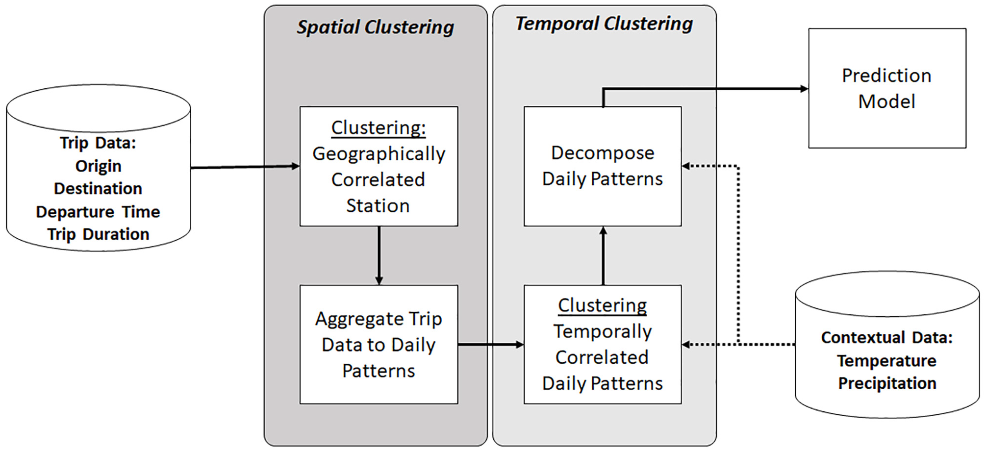
Methodological framework of the proposed low-dimensional approach.

First, trip origins and destinations are clustered in groups of geographically correlated stations. Then, for each cluster, trip data are aggregated—or synthesized—into Vector of Movements. The mathematical details about the process are shown in the next subsection; the difference is that all observations for a specific time interval, such as morning or evening commute, are grouped in one compact vector form (spanned between two spatial points). Temporal clustering will then group them under the assumption that similar vectors lead to similar daily patterns/day type. However, for the same day type, different demand values can be observed. As a consequence, the decomposition process leverages contextual data to find vectors that are consistent across different contextual data, such as precipitation or temperature. Finally, we stress that, if multiple contextual data are available, some of them might be explicitly included within the clustering procedure and the remaining will only be adopted within the decomposition process. In this paper, both options are explored.

In the next subsections, we first describe the two databases (Trip data and Weather data) and then we introduce the four phases of the model.

Data Structure

Trip Data

In this paper, a generic record in the mobility pattern is a trip $T_i$ (Equation 1). Although the complete trip description is complex and might include a full path in space and time, this information is not required in the proposed method, which only requires minimal information in the form of trip origin $O_i$ , destination $D_i$ , start time $t_i$ , and duration $\mathrm{\Delta }{T}_i$ (Equation 1):

$$T_i=\{O_i,D_i,t_i,\mathrm{\Delta }{t}_i\}$$

(1)

Trips recorded over a given time period (day, hour, or week) form a set of observations (Equation 2). Equations 1–2 represent the input for the proposed low-dimensional framework.

$$M_i=\{T_1,T_2,...,T_n\}$$

(2)

Weather Data

In this paper, the term contextual data refers to all data sources that can be used to classify events. These include, but are not limited to, data about weather conditions, special events, public transportation strikes and any information that can be used to understand typical and atypical behaviors in the system. As different contextual data might have different structures, this subsection only describes how to process weather-related databases. Yet, other data could be used with the proposed approach.

In this work, we use daily statistics about precipitation levels and temperature to estimate the demand for BSS. We average and classify the data and assign each observation with its temperature and precipitation class, as shown in Equation 3:

$$C^{{\mathrm{\Theta }}_c}=\{{\mathrm{\theta }}_{\mathrm{low}}<{\mathrm{\theta }}_i⩽{\mathrm{\theta }}_{\mathrm{up}}:i\in {\mathrm{\Theta }}_c)$$

(3)

where ${\mathrm{\theta }}_i$ is the temperature, $C^{{\mathrm{\Theta }}_c}$ represents the subset of observations belonging to the temperature class ${\mathrm{\Theta }}_c$ , and ${\mathrm{\theta }}_{\mathrm{low}}$ and ${\mathrm{\theta }}_{\mathrm{up}}$ are the minimum and maximum average temperature for that class. The same procedure can be applied for precipitation data, obtaining:

$$C^{P_c}=\{P_{\mathrm{low}}<P_i⩽P_{\mathrm{up}}:i\in P_c)$$

(4)

where $C^{P_c}$ represents the group of observations $M_i$ with similar precipitation levels, $P_i$ represents the average precipitation on a given day, $P_{\mathrm{low}}$ and $P_{\mathrm{up}}$ represent the upper bound and lower bound for the class $P_c$ .

Spatial Clustering

As mentioned in the introduction, this study aims at predicting the demand for a certain cluster of BSS stations. Generalizing, we want to identify BSS trips that are spatially correlated and use them to approximate traffic analysis zones (TAZs). Demand from one TAZ to all the others can then be estimated through the framework presented in Figure 1. To do so, we use the Euclidean distance between coordinates to measure the similarity between trip origins coordinates. This creates sub-optimal solutions, as it does not consider accessibility barriers such as rivers or motorways. However, this approach represents the worst-case scenario, as a more realistic similarity measure will generate better clusters and thus better estimations. To this end, we tested the following techniques: Affinity Propagation, Agglomerative Clustering, Gaussian Mixture, and Mean Shift. We exploited the implementation proposed in Scikit-learn, which is an open-source library developed in Python ( 26 ). For the propose of this study, the Gaussian Mixture model clearly outperformed all other models and provides more realistic TAZs when only the Euclidean distance is used as a similarity measure. The procedure returns the following result:

$${\mathrm{TAZ}}_i=\{T_1,T_2,...,T_n\}$$

(5)

where $\mathrm{TAZ}$ is the list of spatially correlated trips $T$ .

Aggregate Trip Data: Vectors of Movements

Daily mobility patterns are composed of thousands of trips per day, each of them characterized by various data including trip origin, destination, and duration. It is far from obvious when two mobility patterns present similar characteristics.

We presume that fundamental set features such as trip duration and cardinality are not sufficient to identify mobility pattern similarities. In addition, if all these features were to be explicitly modeled the dimension of the BSS demand forecasting problem would quickly increase. Therefore, we propose a new way of representing mobility patterns. We start from the concept of gravity center (mass center), an arithmetic mean of trip origins, destinations, or both. Then we introduce Vector of Movements spanning between them. Because of the particular meaning of peak hours in the mobility patterns, we introduce a vector for AM and PM peak hours.

For a generic traffic zone $\mathrm{TAZ}$ , we indicate with $M^{\mathrm{TAZ}}$ the mobility pattern with all trips generated/attracted by the zone. Then, we introduce center of gravity for origins (Equations 6, 8) and destinations (Equations 7, 9). Specifically, Equations 6 and 7 represent the center of gravity for the origin/destination points located within the $\mathrm{TAZ}$ . Similarly, Equations 8 and 9 indicate the center of gravity for origin/destination points located outside the traffic zone $\mathrm{TAZ}$ . The vector spanning between them is the Vector of Movements (Equation 10).

$$O_M^{\mathrm{TAZ}}=E(O_i:i\in M^{\mathrm{TAZ}},i\in \mathrm{TAZ})$$

(6)

$$D_M^{\mathrm{TAZ}}=E(D_i:i\in M^{\mathrm{TAZ}},i\in \mathrm{TAZ})$$

(7)

$$O_M=E(O_i:i\in M^{\mathrm{TAZ}},i\notin \mathrm{TAZ})$$

(8)

$$D_M=E(D_i:i\in M^{\mathrm{TAZ}},i\notin \mathrm{TAZ})$$

(9)

$$\overrightarrow{V}=\{\begin{array}{cc}\overleftarrow{O_M^{\mathrm{TAZ}}{D}_M},\hfill & {\mathrm{if}|\mathrm{O}}_{\mathrm{M}}^{\mathrm{TAZ}}|⩾{|\mathrm{D}}_{\mathrm{M}}^{\mathrm{TAZ}}|.\hfill \\ \multicolumn{1}{c}{\overleftarrow{O_M{D}_M^{\mathrm{TAZ}}},}& \mathrm{otherwise}.\hfill \end{array}$$

(10)

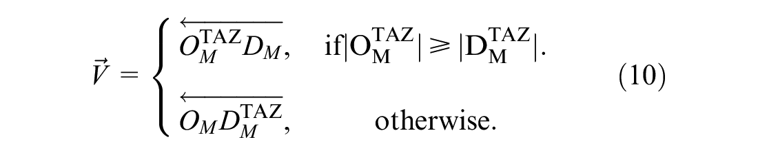
From the daily mobility, we analyze trips of the $\mathrm{AM}$ and $\mathrm{PM}$ peaks. Peaks are identified as the average temporal profile between the two busiest morning and afternoon hours. From the mobility pattern two subsets are selected: $M_{\mathrm{AM}}^{\mathrm{TAZ}}=\{T_i:T_i\in M^{\mathrm{TAZ}},t_i\in \mathrm{AM}\}$ , and $M_{\mathrm{PM}}^{\mathrm{TAZ}}=\{T_i:T_i\in M^{\mathrm{TAZ}},t_i\in \mathrm{AM}\}$ . In fact, the above mapping transforms any number of trips into four points: AM origin and destination, PM origin and destination. Such interpretation synthesizes all main characteristics of mobility patterns (Equation 11).

$$M^{\mathrm{TAZ}}\to \{{\overrightarrow{V}}_{\mathrm{AM}},{\overrightarrow{V}}_{\mathrm{PM}}\}$$

(11)

Note that, in the case of station-based BSS, the clustering is performed on the station ID, so (Equation 10) is calculated by taking into account the direction of the demand (there are more trips generated or attracted in the zone). In the case of free-floating services, in which the spatial clustering is performed on the trip ID, the two vectors are the same and are calculated under the assumption that $|O_M^{\mathrm{TAZ}}|⩾|D_M^{\mathrm{TAZ}}|$ , as all trip origins are within the cluster whereas destinations might be inside or outside the TAZ.

Temporal Clustering

To cluster Vectors of Movements and Weather Data, we need to specify proper similarity measures and a clustering technique. Both are described in this subsection.

The main advantage of synthesizing trips in vectors is that VM allows for pairwise comparison of days/observations, which is troublesome for a set of recorded trips. We propose to compare two generic vectors $\overrightarrow{V}$ and $\overrightarrow{V}\prime$ with a cosine similarity (Equation 12) which returns similarity from range 0 to 1, 1 for vectors with the same direction and 0 for orthogonal vectors.

$$S(\overrightarrow{V},\overrightarrow{V}\prime )=\frac{\overrightarrow{V}·\overrightarrow{V}\prime }{|\overrightarrow{V}||\overrightarrow{V}\prime |}$$

(12)

The cosine similarity shown in Equation 12 could directly be used on the VM introduced in the previous subsection. However, this procedure would only measure the similarity in relation to direction. Instead, we propose to calculate the similarity in a three-dimensional space, thus introducing the following modified vector:

$${\overrightarrow{V}}^{3D}=\{\begin{array}{cc}\overleftarrow{O_M^{\mathrm{TAZ}}{D}_M\mathrm{\Delta }{L}_{\overrightarrow{V}}},\hfill & \mathrm{if}|O_M^{\mathrm{TAZ}}|⩾|D_M^{\mathrm{TAZ}}|.\hfill \\ \multicolumn{1}{c}{\overleftarrow{O_M{D}_M^{\mathrm{TAZ}}\mathrm{\Delta }{L}_{\overrightarrow{V}}},}& \mathrm{otherwise}.\hfill \end{array}$$

(13)

where $\mathrm{\Delta }{L}_{\overrightarrow{V}}={\overrightarrow{V}}_{\mathrm{Length}}-\overrightarrow{V}{\prime }_{\mathrm{Length}}$ is the difference in the length of the two vectors. When comparing $\overrightarrow{V}$ and $\overrightarrow{V}\prime$ , $\mathrm{\Delta }{L}_{\overrightarrow{V}}$ is always 0 for one of the two vectors ( $\overrightarrow{V}\prime$ ) and equal to the difference between ${\overrightarrow{V}}_{\mathrm{Length}}-\overrightarrow{V}{\prime }_{\mathrm{Length}}$ for the other one. We can then apply the similarity measure (Equation 12) to ${\overrightarrow{V}}^{3D}$ to capture both direction and distance in one compact similarity index.

Consequently, we can introduce the pairwise distance measure between two days N and M. Given the Vectors of Movements for the morning and evening commute, calculated as in Equations 10, 11, and 13, the similarity between the two days is given by:

$$\begin{array}{c}\begin{array}{c}\begin{array}{c}\multicolumn{1}{c}{d(N,M)=\mathrm{\alpha }·S({\overrightarrow{M}}^{\mathrm{AM}},{\overrightarrow{N}}^{\mathrm{AM}})+}\\ (1-\mathrm{\alpha })·S({\overrightarrow{M}}^{\mathrm{PM}},{\overrightarrow{N}}^{\mathrm{PM}})\hfill \end{array}\hfill \end{array}\hfill \end{array}$$

(14)

where $S({\overrightarrow{M}}^{\mathrm{AM}},{\overrightarrow{N}}^{\mathrm{AM}})$ and $S({\overrightarrow{M}}^{\mathrm{PM}},{\overrightarrow{N}}^{\mathrm{PM}})$ are the similarities between morning and evening VMs, respectively, and $\mathrm{\alpha }$ is a normalized weight, treated as a parameter of the procedure (we use default $\mathrm{\alpha }=0.5$ in the case study, which can be adjusted to put more weight on morning and evening, respectively). If contextual data are directly combined with cosine similarity to obtain a pairwise distance that takes into account both day type and weather condition, Equation 14 becomes:

$$\begin{array}{c}\begin{array}{c}\begin{array}{c}d(N,M)={\mathrm{\beta }}_1·[\mathrm{\alpha }·S({\overrightarrow{M}}^{\mathrm{AM}},{\overrightarrow{N}}^{\mathrm{AM}})+\hfill \\ (1-\mathrm{\alpha })·S({\overrightarrow{M}}^{\mathrm{PM}},{\overrightarrow{N}}^{\mathrm{PM}})]-\hfill \\ \sum _i{\mathrm{\beta }}_i·S({\mathrm{\lambda }}_i^M,{\mathrm{\lambda }}_i^N)\hfill \end{array}\hfill \end{array}\hfill \end{array}$$

(15)

where $\mathrm{\beta }$ are weights assigned to each component depending on the trust that one has on the data, $S({\mathrm{\lambda }}_i^M,{\mathrm{\lambda }}_i^N)$ represents the similarity between contextual data, and ${\mathrm{\lambda }}_i^M$ is the class for data type i and day $M$ . In this case, it represents the temperature and precipitation class. This similarity is calculated as:

$$S({\mathrm{\lambda }}_i^M,{\mathrm{\lambda }}_i^N)=\frac{|{\mathrm{\lambda }}_i^M-{\mathrm{\lambda }}_i^N|}{{\mathrm{\lambda }}_i^N}$$

(16)

Such metric can be applied to most clustering methods. Note that a 0 value means a perfect match, whereas errors return positive values. This is why ${\mathrm{\beta }}_i$ has a negative sign in Equation 15. Finally, the clustering procedure exploits these similarity measures to create a cluster membership map, that is, it associates each day with a cluster $c(M_i)$ , which is the subset of days with a similar daily mobility pattern $C=\{M_i:c(M_i)=C\}$ . In this research, we apply the agglomerative hierarchical clustering algorithm. Yet, any alternative method can be applied.

Decomposition

If a sufficient number of observations is available, results from the clustering procedure can be adopted to forecast the mobility demand $M_e$ for the current cluster and associated day-types (working day, holiday, etc.) with Equation 17.

$$M_e=E(M_i:i\in C)$$

(17)

However, if not all information has been included within Equation 15, the model is likely to provide a biased estimation $M_e$ . We thus include this information—temperature and precipitation in this case—after the clustering to avoid inconsistent results while keeping the number of parameters low.

To account for the contextual information, we exploit the classes already introduced in the subsection Data Structure: Weather Data. As each day is associated with a specific temperature/precipitation class, the input data are already divided into subsets of homogeneous observations $C^{{\mathrm{\Theta }}_c}$ and $C^{P_c}$ . Thus, the decomposition will divide available information by taking into account that similar observations need to be consistent for both cluster groups and weather/precipitation class:

$$C^{*}=C\cap C^{{\mathrm{\Theta }}_c}\cap C^{P_c}$$

(18)

with $C^{*}$ being the optimal cluster, which is consistent according to all the available data. The estimation model will then be:

$$M_e=E(M_i:i\in C^{*})$$

(19)

which provides the most likely mobility pattern for a given cluster and temperature. In particular, for each TAZ we obtain the expected vector $V$ representing in aggregated form trips to/from a given zone, obtained as a mean of clustering.

Remarks

As we will show in the next section, this methodology performs particularly well in combining contextual and trip data (Vectors of Movements) to identify recurrent mobility patterns. However, the ultimate goal is to forecast hourly rental rates at a zonal level. The hourly prediction for a certain cluster of observations can be obtained as the average rental rate of the observations belonging to the cluster ( 21 ). However, as our data are divided into two parts—training and test points—we also need to associate each test point to a cluster. This is a crucial aspect, as associating training points to the wrong cluster would provide highly inaccurate predictions. To avoid this problem, we use categorical variables to label our data before the clustering. For instance, each day is labeled as “working day” or “holiday,”“warm” or “cold.” These labels are used to match each test point to a unique cluster.

Concerning the generality of the model, the proposed methodology can be applied to both free-floating and dock-based systems. However, the main difference between the two systems lies in the spatial-clustering phase. Creating TAZ from station IDs is a relatively trivial task. However, creating TAZ for a free-floating system might call for another clustering itself, in which exact bicycle locations are clustered spatially. In both cases, a poor spatial clustering would result in poor model performances.

Finally, although this procedure returns accurate predictions of daily patterns, it should be stressed that it does not provide insights in relation to policy analysis. On the other hand, contextual data can be used to identify factors influencing the mobility demand. For example, our results from the New York case study show that temperature data should be included within the estimation framework, as they help the model to better explain the demand. This is in line with previous findings ( 10 ), which showed that, in New York, weather affects cycling rates more than topography, infrastructure, land-use mix, calendar events, and peaks.

Validation: The Case of New York City

The procedure illustrated in the previous section is now validated on real-world data to assess its applicability. To this aim, we collected and processed trip data for the year 2018 (over 17 millions bike trips) from Citi Bike (New York City), one of the biggest BSS in the United States. City Bike NYC is a station-based BSS with more than 15,000 bikes in New York City and Jersey City, New Jersey. Basic statistics are presented in Table 1.

Table 1.

Citi Bike Database: 2018.

Last day	31/12/2018
First day	01/01/2018
Number start stations IDs	3.315
Number of bikes	15.244
Number of trips	17.548.339
Statistics
Number of daily trips (avg.)	47.575
Number of daily trips (max.)	79.336
Number of daily trips (min.)	1.893
Temperature (°F) (min./avg./max.)	9.5/55.9/87.5
Precipitation ( $100\mathrm{in}$ .) (min./avg./max.)	0/0.2/2.9
Number of rainy days (precipi. $>0.1$ )	94/365

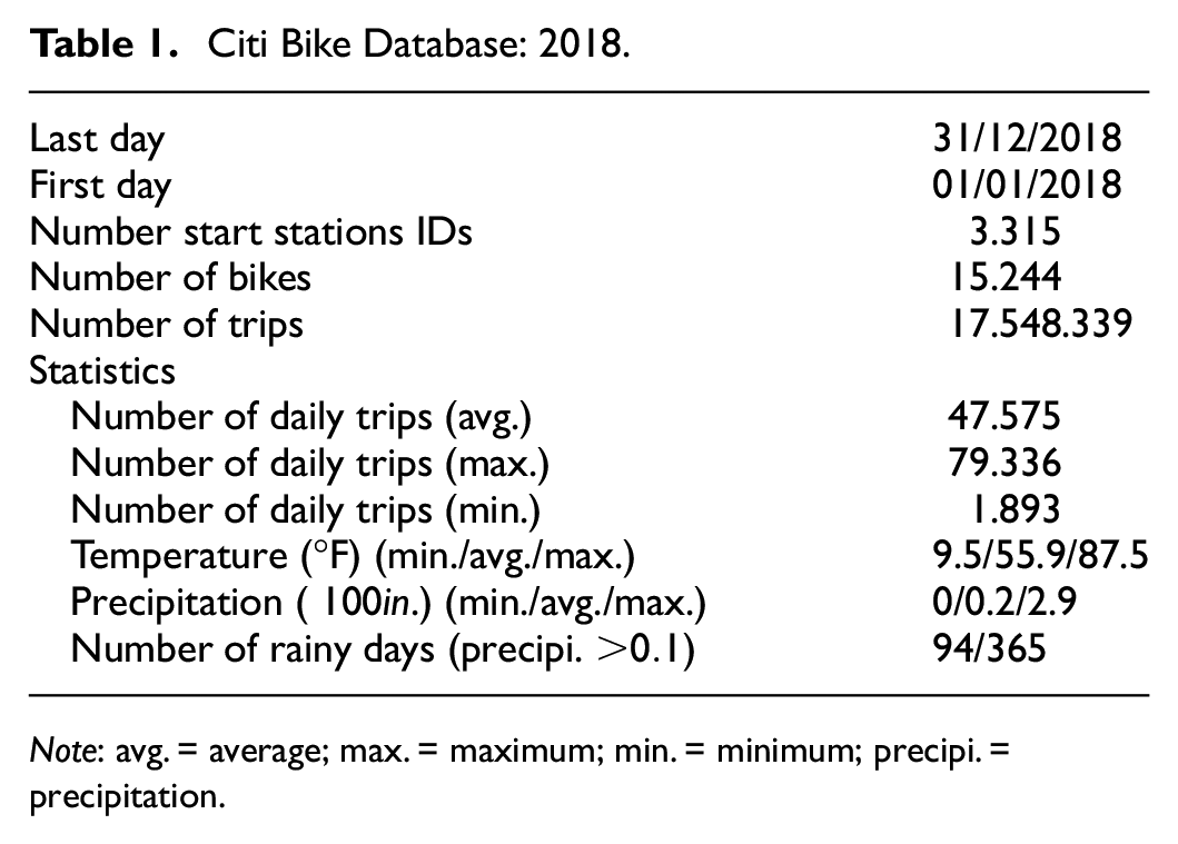
Note: avg. = average; max. = maximum; min. = minimum; precipi. = precipitation.

General statistics show the volume and complexity of the available database. The average daily number is in fact about 45,000 trips, but this number shows a large variance.

Vectors of Movements: A Sensitivity Analysis

To validate the proposed model and to support our claims, we perform in this section a sensitivity analysis for the temporal clustering. Specifically, we use Equations 14 to compare the predictions at a daily and cluster level. We also compare results when using $\overrightarrow{V}$ or ${\overrightarrow{V}}^{3D}$ within the clustering procedure. The advantage is that we can perform a sensitivity analysis for only one input variable—the number of clusters—and we can analyze how the model performs at a cluster level with and without ${\overrightarrow{V}}^{3D}$ . This is also a first comparison with the previous model ( 20 ), as Equation 13 is a generalization of the first VM (20). The new version can, in fact, be applied to clusters, and not only at a city level, and it is sensitive to generation and attraction volumes. Similarly, the proposed ${\overrightarrow{V}}^{3D}$ is a generalization that introduces more information within the standard VM. Although this concept can be extended to $n$ -dimensions, before introducing additional measures this metric needs first to be validated. This is the main contribution of this section. Validating the quality of a clustering procedure is a challenging task, as different metrics point out to different results. Thus, the database has been divided into two parts: 75% of the data are used for training the model and the remaining 25% of the database is used for validation. Both internal and external validation measures are applied.

• Internal cluster validation: Evaluates the goodness of a clustering structure without reference to external information. Internal verification should measure cluster Compactness and Separation. The first indicates how closely related are the objects within a cluster, whereas the second indicates how well separated clusters are ( 27 ).

• External cluster validation: Evaluates the “purity” of the procedure by comparing it with external information, not available within the clustering procedure.

In this study, we use the Silhouette Index and the Calinski–Harabasz Index for internal validation, which balance compactness and separation performances ( 27 ). For the external validation, we calculate clusters’ entropy to the validation dataset. Specifically, the Silhouette value ranges from $-1$ to $+1$ , where $+1$ indicates a perfect match. Similarly, for the Calinski index, higher values translate into a better match. We refer to Liu et al. for a detailed overview of these metrics ( 27 ).

Finally, to calculate the entropy of the system, we calculate the Shannon entropy index for each cluster:

$$H_i=-\sum _{j\in K}p(i_j)\underset{2}{\log }p(i_j)$$

(20)

where $H_i$ represents the entropy level for cluster $i$ and $p(i_j)$ is the probability that observation in class $i$ is classified in a different class $j$ . If all objects are properly classified, Equation 20 becomes $(-1\underset{2}{\log }1)$ and the entropy for cluster $i$ is zero, which is the best solution. Given the entropy for class $i$ , the entropy of the system $H$ is given by Equation 21:

$$H=\sum _i{H}_i\frac{N_i}{N}$$

(21)

with $N_i$ the number of elements in class $i$ and $N$ the total number of observations. Again, low values of $H$ means a better clustering, with 0 the best match between the prediction model and data.

Results of the sensitivity analysis are depicted in Figure 2. Specifically, Figure 2, a and b , show two possible zonal clusterings. As specified in the previous section, we adopted the Gaussian Mixture algorithm as it provides better results. Figure 2, c–e , show instead the internal/external verification of our proposed approach at a city level, at a cluster level, and when the ${\overrightarrow{V}}^{3D}$ is combined in Equation 15. The same analysis has been performed for different traffic zones, but for practical reasons, we only show the results for TAZ 1, which provides average performances with respect to all the proposed zones.

Figure 2.

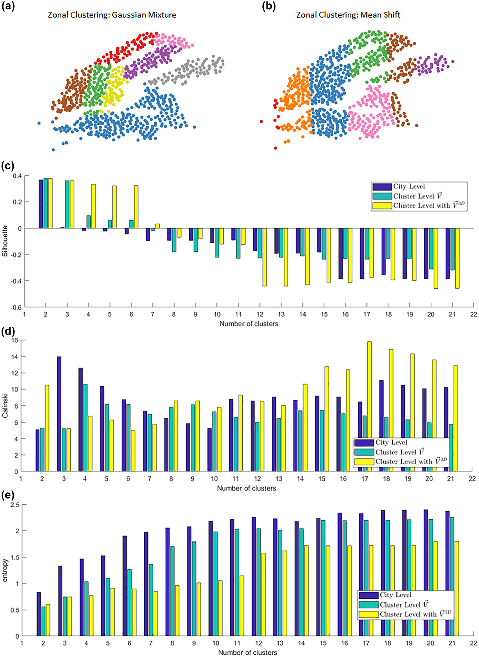
Sensitivity analysis at city level and cluster level: (a) zonal clustering with Gaussian Mixture, (b) zonal clustering with Mean Shift, (c) values of the Silhouette Index, (d) values of the Calinski–Harabasz Index, (e) values for the entropy.

By looking at the difference between city-level predictions and cluster-level predictions, we can see that the model is usually performing better at a cluster level. Specifically, with respect to the entropy—which is the most reliable measure—the model systematically outperforms the city-level one. Concerning the Silhouette and Calinski–Harabasz indexes, the analysis is not straightforward. For the Silhouette, cluster-level predictions usually provide better estimations for a low number of clusters (between 2 and 7) and perform worse for a larger number. On the contrary, the city level works better for a low number of clusters according to the Calinski–Harabasz index. As pointed out in the literature ( 27 ), the Silhouette index provides biased estimations when many sub-clusters exists (i.e., two different clusters are grouped in a single one). The Calinski–Harabasz is instead very sensitive to noise in the data. As the database at city level aggregates millions of trips in a few clusters, the index still returns a good value even if both entropy and Silhouette point to the opposite solution. This suggests that we need to find clusters that are consistent across the three metrics. This becomes easier when the ${\overrightarrow{V}}^{3D}$ is used within the clustering. By filtering the noise, the model systematically outperforms all the others in relation to entropy, provides better Silhouette results for several clusters between 2 and 9, and better value for the Calinski–Harabasz when the number of clusters is larger than 7. This indicates that the optimal number of clusters should be between 7 and 11. However, we can notice that for both Entropy and Silhouette results are systematically better for low numbers of clusters. Again, this is related to the structure of the index. As already mentioned, Silhouette is not sensitive to sub-clusters, meaning that it returns high values when different clusters are grouped together, which is the situation for several clusters equal to 2.

Similarly, the entropy is the most reliable measure to compare our results but, in this case, it is not the best measure to calculate the best number of clusters for a given method, as it is more likely to obtain low values when only two clusters are allowed. However, to assume that only two clusters exist means that for the entire database—more than 17 million trips—we are assuming only two daily patterns while assuming that any deviation from these patterns is unpredictable noise. To avoid this last problem, we also calculated the prediction error in relation to normalized mean absolute error (NMAE). Results are shown in Figure 3 where, for a given number of cluster, the boxplot of all NMAE values is shown. We can see that, when the normal vector of movements is adopted (Figure 3b), results are similar for a small number of clusters and decreases when 12 clusters are used. On the other hand, when ${\overrightarrow{V}}^{3D}$ is adopted, results are systematically lower in relation to both mean and variance. As shown in Figure 3a, results are systematically better (up to two times) for several clusters between 7 and 12, showing that the proposed metric does indeed reduce the noise in the results, thus providing results that are more consistent according to all proposed metrics.

Figure 3.

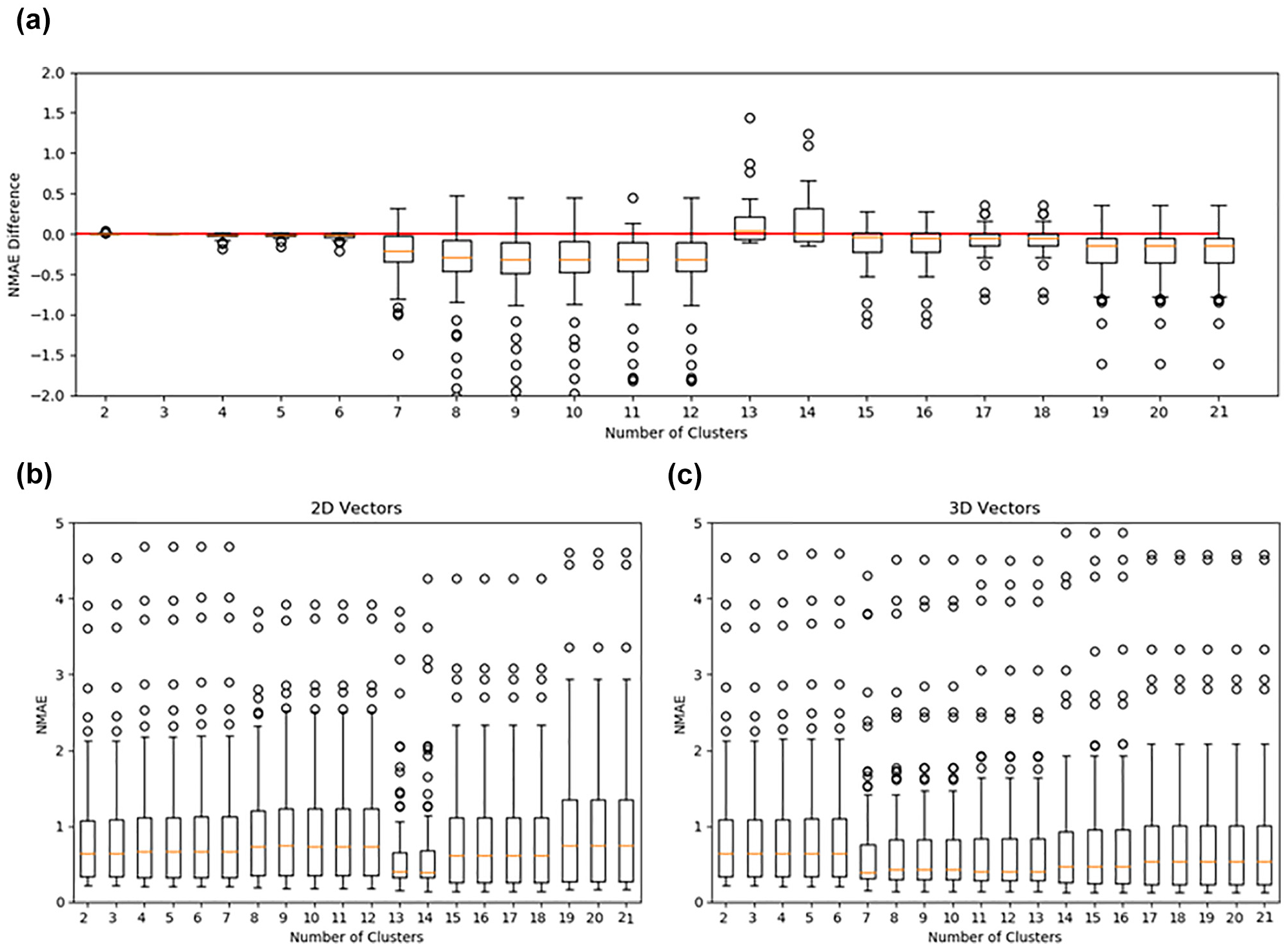
Normalized mean absolute error (NMAE): (a) difference ${\mathrm{NMAE}}_{{\overrightarrow{V}}^{3D}}-{\mathrm{NMAE}}_{\overrightarrow{V}}$ , (b) NMAE for $\overrightarrow{V}$ , and (c) NMAE for ${\overrightarrow{V}}^{3D}$ .

Temporal Clustering with Contextual Data

In this subsection, we analyze the performances of the model when three-dimensional vectors ${\overrightarrow{V}}^{3D}$ and contextual data are combined together. Based on the previous observations, we decided to investigate the performances of the model for several clusters between 5 and 20. The performances of the model are calculated based on two metrics: the root mean squared error (RMSE), which returns the average error in relation to demand flows, and the prediction accuracy. The latter is directly derived from the confusion matrix and calculates the percentage of observations correctly predicted (i.e., properly represented by their cluster). Results are presented in Figure 4, where the red dashed line represents a prediction precision of 75%, which is considered a good result in this study. Four situations have been evaluated:

1. Experiment 1: Only ${\overrightarrow{V}}^{3D}$ are considered within Equation 15 (Figure 4a);

2. Experiment 2: ${\overrightarrow{V}}^{3D}$ and temperature data are used within Equation 15 (Figure 4b);

3. Experiment 3: ${\overrightarrow{V}}^{3D}$ and precipitation data are used within Equation 15 (Figure 4c);

4. Experiment 4: All data are used within Equation 15 (Figure 4d).

Figure 4.

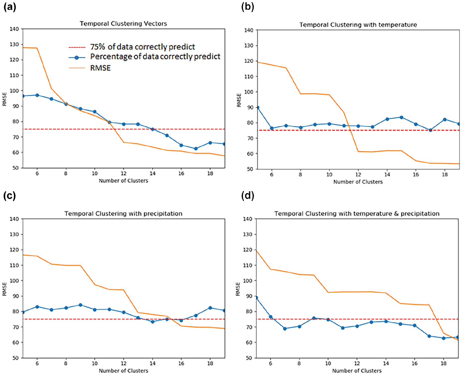
RMSE and precision level for: (a) Experiment 1, (b) Experiment 2, (c) Experiment 3, and (d) Experiment 4.

Results clearly show that best performances are obtained for Experiments 1 and 2. They clearly show a significant reduction of the error and a reasonable precision when increasing the number of clusters. However, for Experiment 1, we can see that the precision decreases almost linearly with the error, meaning that there is a risk of overfitting the data. On the contrary, when weather data are adopted, we can clearly see that the error has a significant reduction for several clusters equal to 12, while the precision of the model stays constant—that is, always above 75%. Similar observations can be done for Experiment 3. However, the RMSE is definitely higher in this case. Finally, Experiment 4 combines all contextual data (weather and precipitations) to forecast the demand (Figure 4d). Both RMSE and precision of the model do not provide satisfactory results, suggesting that—for the current values of ${\mathrm{\beta }}_i$ in Equation 15—combining all contextual data leads to worse results.

Cluster Decomposition

This is the last building block of the proposed framework, where we adopt Equations 18 and 19 to include all the remaining information in the model. We use the same settings proposed in Experiment 1 and 2 before applying the decomposition scheme, as these provided the best results. Results are depicted in Figure 5. Specifically, Figure 5a represents the results for Experiment 1 and Figure 5b shows the results for Experiment 2. The overall time to perform one estimation of the model is a few minutes on a normal laptop (Intel i7 with 8 GB RAM).

Figure 5.

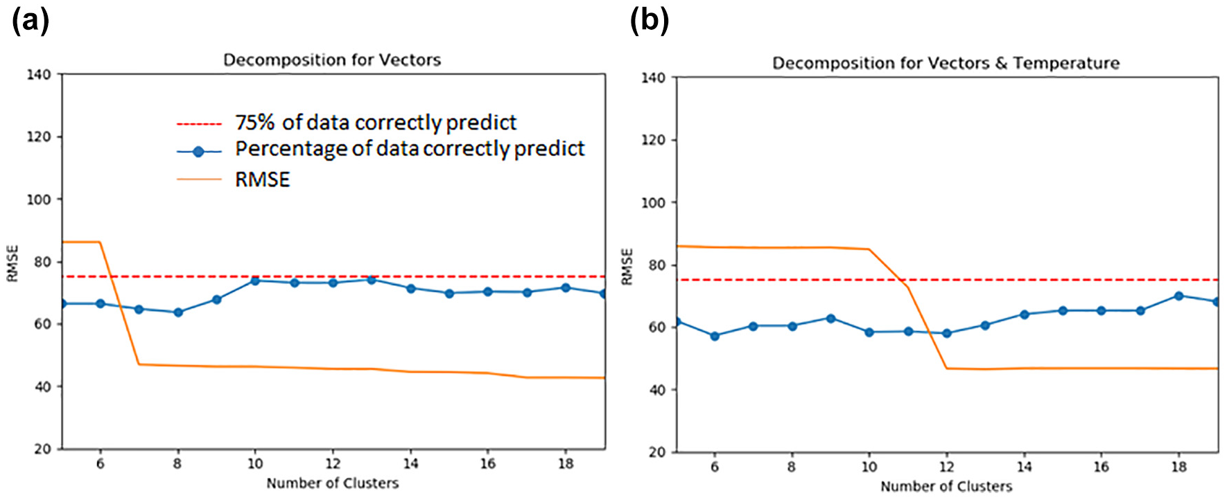
RMSE and precision level when applying the decomposition scheme to: (a) Experiment 1 and (b) Experiment 2.

The first observation that should be reported is that the model shows very stable results in relation to both RMSE and precision. However, both indexes are definitely lower than those obtained in the previous section. This means that the decomposition scheme allows the model to do some overfitting of the data, which might not be an ideal solution. Despite that, the precision results are relatively high (between 60% and 75%) for both models. In addition, the best performances are obtained when only VMs are used within the clustering procedure and all contextual data are adopted in the decomposition phase (number of clusters = 12, precision ≌ 75%). Finally, it is interesting to point out that the decomposition scheme clearly shows different performances with the increasing number of clusters. The difference is observed for several clusters equal to 7 (Experiment 1) and 12 (Experiment 2). According to all metrics adopted, when only vectors of movements are considered, good results can only be obtained for more than seven clusters, meaning that this is the minimum number of cluster to properly identify daily mobility patterns in our study.

However, when we cluster using mobility patterns and weather data, the model needs to classify each daily activity patterns according to two pieces of information, so the optimal number of cluster is almost twice the one of Experiment 1. When the daily patterns have been properly classified, then the decomposition scheme is capable of providing a significant improvement in relation to RMSE.

Finally, we stress that in both cases the proposed decomposition scheme is performing better than Experiment 4, introduced in the previous subsection, in which both precipitation and temperature data were included in the clustering procedure.

Conclusion

In this paper, a low-dimensional model for BSS demand forecasting has been proposed. The framework clusters BSS trips at a spatial and temporal level to predict the mobility demand for a certain cluster/zone. Compared with conventional clustering approaches, our framework includes two additional phases, named Aggregation and Decomposition, which aim at reducing the complexity of the problem. The Aggregation phase synthesizes all trips in a compact form, called Vectors of Movements (VM). This compact form keeps most of the characteristics of the original demand while allowing for simple pairwise comparisons of daily patterns, which was not possible with disaggregated trips. The decomposition scheme allows instead the introduction of contextual data—temperature and precipitation in this study—to achieve more accurate predictions while keeping the overall number of variables low. The work presented in this paper is an extension and generalization of the model presented in Cantelmo et al. ( 20 ), which used VM to estimate the demand at a city level. Contributions of this paper can be summarized as follows:

1. A generalized version of the Vectors of Movements has been proposed. The new version can be used to estimate hourly rental rates at a cluster/zonal level, and it is sensitive to the attractivity of the zone;

2. A new procedure to calculate N-Dimensional VMs has been proposed. Each additional dimension represents a new level of information that can be included in the vector;

3. A general approach to include contextual data has been proposed. The model can use contextual data both within the clustering procedure, as suggested by other authors, or within the decomposition scheme. This allows accounting for more data while avoiding overfitting issues.

The methodology has been applied to publicly available trip data from the New York City bike system (Citi Bike) to forecast BSS demand at a cluster level. In total, 17 million trips have been processed. Several experiments have been proposed, showing that the model provides reliable results.

Future work will focus on three main research directions: First, to investigate new methodologies for both clustering and prediction, including time-series regression. This will allow us to use this methodology for both real-time predictions and rebalancing procedures. Second, to include land-use and socio-demographic information within the demand forecasting for planning purposes. Third, to test the proposed framework with different mobility services, including free-floating BSS and e-scooters.

Finally, we will analyze limits and opportunities of the vectors of movements. In fact, as they approximate the structure of the demand, they might be sensitive to recurrent behavior but provide less accurate predictions for non-recurrent behavior, if this is not properly represented in the training database.