Sage Journals: Discover world-class research

Abstract

In this paper, a decision support system is proposed to assist an analyst in updating the highway roadside asset inventory. The feasibility of the system is tested with assets along an 8 km section of the A27 highway on the south coast of England, UK. Survey data from a vehicle equipped with a single forward-facing camera and a GPS-enabled inertial measurement unit, aerial imagery of the highway, and the asset inventory are fused to develop the system. The camera on the vehicle is calibrated so that assets may be automatically located within the survey images. The assets are then classified by a state-of-the-art convolutional neural network. Therefore, those assets recorded correctly in the inventory and those needing further manual inspection are automatically identified. Three different asset types are considered (traffic signs, matrix signs, and reference marker posts), and overall 91% of the assets in a withheld test set are verified automatically. Thus the analyst is presented with a much smaller set of assets for which the inventory is incorrect and which require further inspection. We therefore demonstrate the value in fusing multiple data sources to develop decision support systems for transportation asset monitoring.

An operational and safe highway network is critical to daily life, business, and ultimately the economy ( 1 ). Therefore, effective transportation asset management (TAM), defined as “the strategic and systematic process of operating, maintaining, upgrading and expanding physical assets effectively throughout their lifecycle” ( 2 ) is vital. To regulate and implement TAM, highway agencies typically follow practices detailed in a TAM plan (TAMP), constructed by government or national-level departments. For example, highway agencies from the Netherlands, Ireland, Italy, and the UK are currently collaborating with research centers across Europe on the asset monitoring for infrastructure (AM4INFRA) project ( 3 ). The initiative aims to provide an asset management framework to enable “consistent and coherent cross-asset, cross-modal and cross border decision-making,” to ensure standardized, safe, and value-for-money TAM across Europe. Similarly, the U.S. Department of Transportation provides extensive guidance on how to develop an effective TAMP for state agencies ( 4 ).

The process of asset inventory and field data collection is identified as an important step in a TAMP ( 5 ). Typically, the inventory contains geographical, physical, and condition data for each of the assets. Field data may range from manual inspection of the assets to LIDAR point clouds. Reportedly, over 70% of U.S. state agencies survey the highway to collect data on assets such as the pavement, signs, guardrails, and lighting units ( 2 ). However, the development of asset-monitoring systems for high-cost, low-quantity assets has been prioritized because of funding constraints ( 6 ). Instead, for roadside assets, an analyst usually inspects the survey data, and updates the asset inventory manually. Furthermore, in some regions of the UK, it is common for assets to be monitored via physical inspection in which the inventory is updated on site with a ruggedized tablet (Jacobs, personal communication). Consequently, asset monitoring becomes infrequent and costly.

Cameras provide a relatively cheap sensing capability; therefore, imagery data of assets are often collected in surveys. There are many roadside assets, and several reasons why the inventory may be incorrect; for example, the asset may have been moved or damaged between surveys. Therefore, it is difficult for the analyst to comprehensively and accurately maintain the inventory from manual inspection of the images. Thus there is a requirement for tools and systems to assist the analyst in their decision-making when monitoring roadside assets. Furthermore, rich data sources concerning the assets already exist to develop and test the tools.

Usually, the number of assets recorded incorrectly is small compared with those that are correct. Consequently, the analyst spends only a small fraction of their time inspecting those assets that require further attention and updating. Therefore, a decision support system that might automatically identify only those assets that are recorded incorrectly has the potential to reduce the manual workload and improve on the current inventory updating process.

In this paper, one such system that employs computer vision techniques is developed and demonstrated. To prove its feasibility, an inventory of roadside assets installed along an 8 km section of the A27 on the south coast of England is considered. To develop the system, imagery and position data from a survey, captured by a vehicle equipped with a single forward-facing camera, and a GPS-enabled inertial measurement unit (IMU) are used. In addition, data from the asset inventory, and aerial imagery of the highway are also considered. The decision support system is tested on three types of assets: traffic signs, matrix signs, and reference marker posts. In developing this system, we demonstrate the value in fusing multiple data sources to support the TAM decision-making process, and to reduce the workload expected of the analyst. Furthermore, the single camera and IMU represents a cheap and deployable sensing capability. It is envisioned that the system will form a future distributed and ubiquitous monitoring capability, so that assets installed on all national highways may be frequently monitored and easily maintained. To the author’s knowledge, this is the first TAM system that automatically verifies both the asset type and position recorded in the inventory, from a single camera and IMU.

Literature Review

Computer vision can be broadly understood as two distinct problem areas. First, there are techniques that consider the reconstruction of a 3-dimensional scene in a 2-dimensional image (or collection of 2-dimensional images). Models and algorithms described rigorously in Hartley and Zisserman such as the pinhole camera, structure from motion and computation of the projection and fundamental matrices, allow such rich views of the world to be created ( 7 ). Second, there are pattern recognition-based techniques that extract features in images to perform classification via either supervised or unsupervised learning. An overview of this latter problem area is given by Gonzalez and Woods ( 8 ) and Prince ( 9 ). Further, a variety of computer vision techniques employed by intelligent transportation systems are described in Loce et al. ( 10 ).

A great deal of work has been undertaken in applying computer vision for the automatic detection of assets in images. In particular, there is a large body of literature on traffic sign detection and classification in images. Arnoul et al. developed and deployed a Kalman filter-based system to detect roadside assets from their motion relative to a camera installed on a survey vehicle ( 11 ). Further, Greenhalgh and Mirmehdi presented a support vector machine to classify histogram of oriented gradients (HOG) features generated from images of traffic signs ( 12 ). However, state-of-the-art performance is achieved by deep neural networks; the classifiers proposed by Sermanet and LeCun ( 13 ) and Cireşan et al. ( 14 ) achieve, respectively, 99.17% and 99.46% accuracy on the German Traffic Sign Detection Benchmark dataset. However, these systems classify images in which the sign occupies the majority of the image. Improved methods that can detect and classify traffic signs in whole-scene imagery (in the wild) are presented by Zhu et al. ( 15 ) and Kryvinska et al. ( 16 ).

Several systems that also estimate the asset position have been developed. Wang et al. presented a stereo camera system to estimate the position of assets identified in imagery and tested different configurations (one vehicle with two cameras and two vehicles each with one camera) ( 17 ). In addition, Balali et al. proposed a method that leverages Google Street View imagery to map the position of the assets ( 6 ).

Furthermore, methods that perform a dense 3-dimensional reconstruction of the highway and its assets are presented in Golparvar-Fard et al. ( 18 ) and Uslu et al. ( 19 ). These approaches employ structure from motion techniques to generate point clouds purely from imagery. In addition, semantic texton forests are then employed to perform 2-dimensional segmentation of the image, providing asset classification and 3-dimensional mapping at the pixel level. Unfortunately, point cloud generation from imagery is computationally expensive; however, a cheaper LIDAR-based method for highway asset inventory monitoring is presented in Sairam et al. ( 20 ). Examples of three roadside asset management systems in operation are shown in Figure 1.

Figure 1.
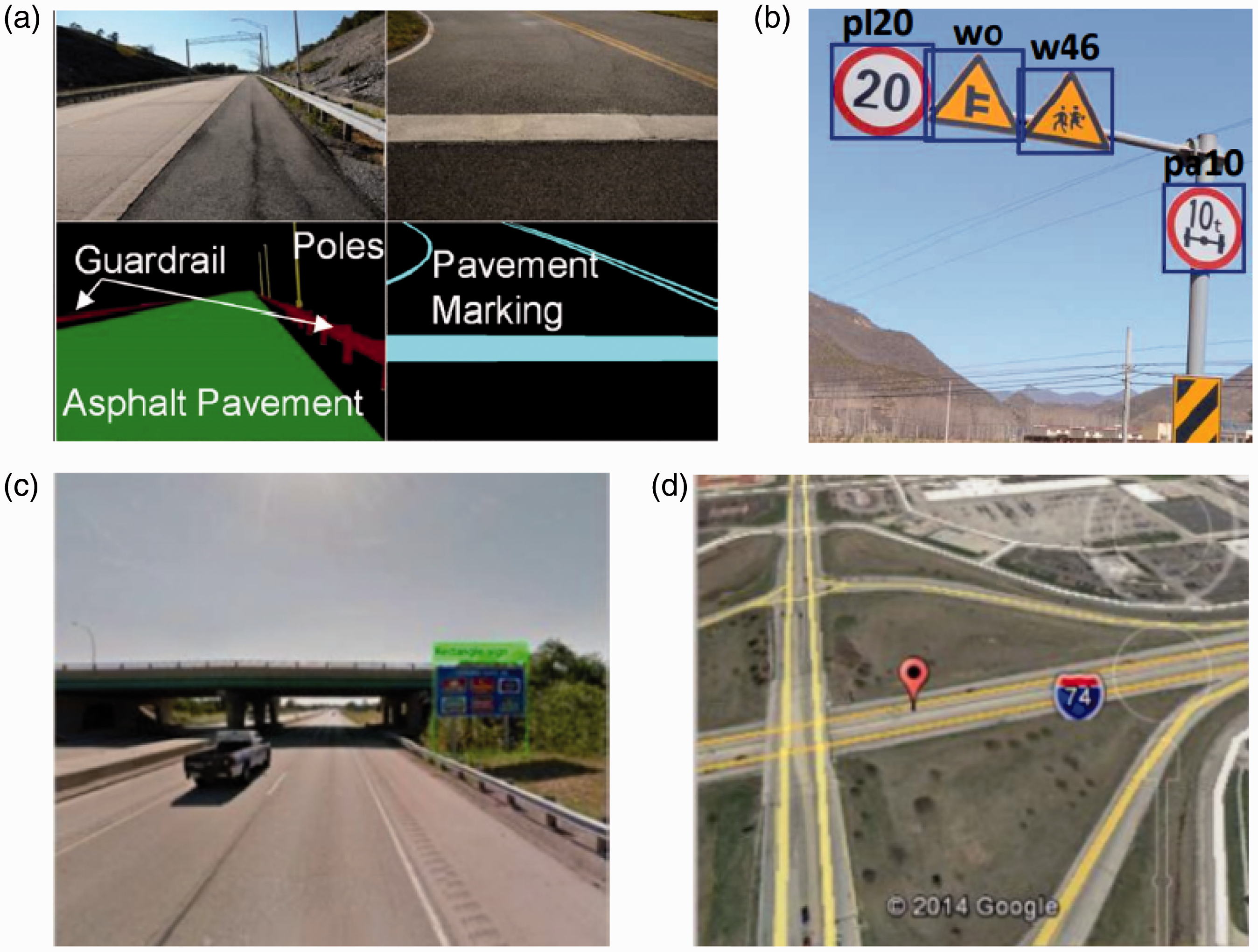
Three existing asset management systems in the literature. Panel (a) shows two examples of the 3-dimensional image reconstruction and asset segmentation described in Golparvar-Fard et al. ( 18 ). Panel (b) shows the labeling exercise undertaken by Zhu et al. ( 15 ). The bounding box and class for each traffic sign is manually collected and used to train a system capable of detecting traffic signs in a whole-scene image of the highway. The system proposed by Balali et al. ( 6 ) is shown in panels (c) and (d). A traffic sign is detected from a Google Street View image, and its position is subsequently computed and mapped.

Further, TAM systems that assess the condition of highway assets have been proposed. Systems that automatically evaluate the retroflectivity of traffic signs, and detect defective road studs (reflective cat’s eyes) are presented, respectively, in Chengbo and Yichang ( 21 ) and Mcloughlin et al. ( 22 ).

In addition to roadside assets, computer vision-based methods have been used successfully to monitor the pavement. Zhang et al. developed a deep learning architecture to automatically identify cracks in images of asphalt pavement at the pixel level ( 23 ). The system is developed and tested on illuminated overhead images of the pavement and thus requires a specialized vehicle to be employed. Similarly, the UK-based company Gaist provides pavement condition data, derived from high-resolution imagery, to highway agencies ( 24 ). From dialog with the company, it is understood that their products do not currently incorporate automation. Rather, they manually label polygons in images with condition data so that future products might be trained to evaluate the highway surface automatically. Gaist also collaborates with the University of York in a project in which refuse trucks are equipped with cameras to monitor the pavement condition ( 25 ). The trucks typically traverse the same routes on a regular basis, and therefore it is hoped that pavement deterioration might be modeled from their data. Other readily deployable pavement monitoring capabilities include the system presented in Radopoulou and Brilakis ( 26 ), which considers imagery data from a parking camera mounted on the bumper of a vehicle.

Data Sources

We now describe the development of our own asset-monitoring decision support system. We first describe each of the data sources that we use. Samples of the data sources are illustrated in Figure 2.

Figure 2.
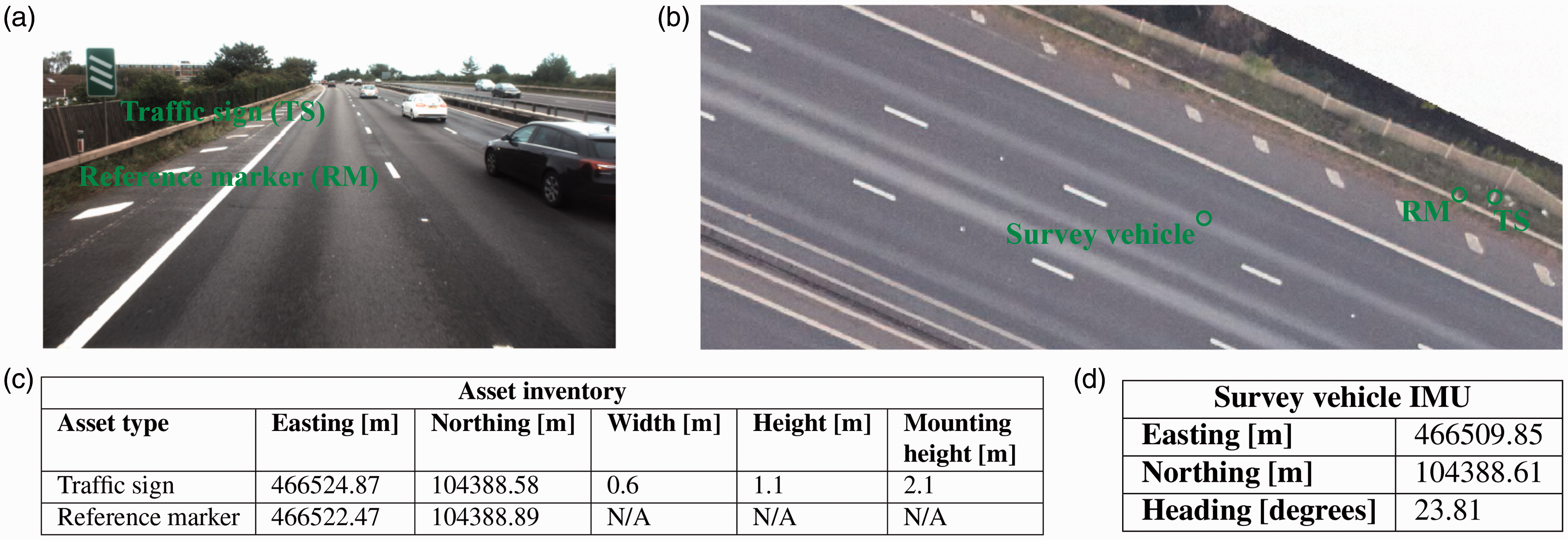
Samples of the data sources used to develop the asset-monitoring decision support system. Panel (a) shows an image of a traffic sign and a reference marker on the highway taken by the forward-facing camera on the survey vehicle. The inventory entries for the two assets are shown in panel (c), and the vehicle position and heading provided by the inertial measurement unit are shown in panel (d). Panel (b) shows an example of the aerial imagery of the highway. This data source provides a view of the A27 in the (e, n) plane, and may be used to find the coordinates of assets and road markings on the surface of the highway. The position of the survey vehicle as the image shown in panel (a) is taken, and the two assets are marked on the aerial imagery.Note: IMU = inertial measurement unit.

Asset Inventory

The asset inventory in the UK must adhere to standards set by Highways England ( 27 ) and contains information such as the asset position, condition, installation date, and maintenance history. However, TAM is often performed by subcontractors, and consequently the inventory can be inaccurate and inconsistent. The position, as a UK Ordnance Survey Easting–Northing coordinate (e, n) ( 28 ), of each asset is recorded in the inventory. For some assets, physical attributes such as the size (width and height) and the mounting height are also provided. For example, the sizes of traffic signs and matrix signs are recorded in the inventory, but the size of the reference marker posts are not. Therefore, the reference markers are assumed to have a 1 m height, 0.5 m width and 0 m mounting height. In total, 590 individual assets (373 traffic signs, 172 reference markers, and 45 matrix signs) are taken forward to develop and test the system.

Aerial Imagery

Overhead imagery of the highway can be viewed using software tools such as ArcMap. The Easting–Northing coordinate for any point on the highway can be obtained from the software; however, the software provides no height relief.

Survey Vehicle

The vehicle is equipped with a GPS-enabled IMU and a single forward-facing camera. As the survey is performed, an image is taken every 2 m along the highway. Simultaneously, the vehicle’s heading angle and position are recorded by the IMU. Thus, each image is accompanied with metadata describing the position and direction of the vehicle as the image is taken. The vehicle’s position as an Easting–Northing (e, n) coordinate and its heading are recorded with a resolution of 0.01 m and $0.01 °$ , respectively.

Data Pre-Processing

The position of each asset is given in the world coordinate system (e, n, z) where z is the height above the highway surface. However, the decision support system considers the assets as viewed by the camera on the vehicle. Therefore, the survey data are processed so that we may consider the assets relative to the vehicle.

Coordinate Transformation

We first define a coordinate transformation of the arbitrary coordinate $p = {(e_{p}, n_{p}, z_{p})}^{⊤}$ in the world frame, to a coordinate $p_{v} = {(x_{v}, y_{v}, z_{v})}^{⊤}$ relative to the IMU on the vehicle, where the x-coordinate axis points along the heading direction of the vehicle, the y-coordinate axis points orthogonally across the width of the highway, and the z-coordinate axis continues to point vertically upwards. The coordinate transformation is achieved by a translation so that the IMU is at the origin of (e, n) plane, and a rotation through the vehicle heading angle θ, about the z-coordinate axis. Therefore, the coordinate relative to the vehicle is given by $p_{v} = R_{z} (p - o_{v})$ , where $R_{z}$ is the 3-dimensional rotation matrix about the z-coordinate axis through the heading angle ( 29 ). The translation vector $o_{v} = {(e_{v}, n_{v}, 0)}^{⊤}$ is the origin of the new coordinate system, and lies directly beneath the IMU on the highway surface, see Figure 3. The coordinates e_v and n_v are the Easting and Northing coordinate recorded by the IMU, respectively. The position of the assets relative to the vehicle may then be computed by this transformation.

Figure 3.
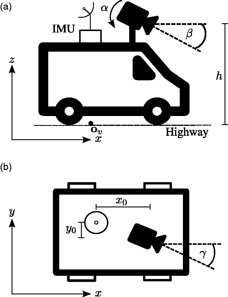
An illustration of the inertial measurement unit (IMU) and camera on the vehicle. Panel (a) shows the vehicle in the (x, z) plane. The IMU and camera are positioned on the vehicle at a height h above the highway surface. The camera has a roll angle α and tilt angle β. The origin of the coordinate system relative to the vehicle, $o_{v}$ , lies directly underneath the IMU on the highway surface. Panel (b) shows the offset of the camera relative to the IMU (x_o, y_o) and the camera’s pan angle γ in the (x, y) plane.

Heading Correction

The heading direction is computed by the IMU in real time from the straight line between the vehicle’s current position and its position as the previous image was taken. The heading angle is then defined as the angle between the heading direction and the Easting coordinate axis. This method is inaccurate when the vehicle turns a corner, and therefore we re-compute the headings after the survey. Specifically, we compute the vehicle’s heading direction as the $i th$ image is taken by using a central difference scheme applied to the position of the vehicle when the $(i - 1) th$ and $(i + 1) th$ image are taken. Our corrected heading angle is thus given by
$θ_{i} \approx \arctan (\frac{n_{i + 1} - n_{i - 1}}{e_{i + 1} - e_{i - 1}})$
(1)

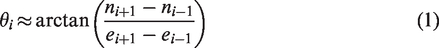
This scheme provides a better approximation for the heading compared with the IMU value that is computed in real time.

Camera Calibration

Shortly we will automatically locate assets within the survey images. This is achieved by calibrating the camera on the vehicle, such that the pixel coordinates of an asset in an image from the survey may be computed, given the position of the asset relative to the camera.

Formally, during camera calibration, we aim to recover the camera parameters that project the arbitrary coordinate $p_{v}$ to a pixel coordinate (u, v) on an image taken by the camera. The camera parameters are categorized into intrinsic parameters; that is, internal properties of the camera, and extrinsic parameters; that is, how the camera is positioned and orientated on the vehicle relative to the IMU.

It is likely that different surveys will use different cameras, which may be installed onto the vehicle in several configurations. Consequently, we may not make any assumptions about the camera or its position and orientation on the vehicle in the survey considered in this paper. Therefore, to locate the assets within the survey images, all intrinsic and extrinsic camera parameters must be calibrated.

Camera Model

Both the IMU and camera are positioned on the vehicle at height h. The camera is offset from the IMU at position $(x_{0}, y_{0}, h)$ and has roll angle α, tilt angle β and pan angle γ; namely, rotations about the x-coordinate, y-coordinate and z-coordinate axis respectively, shown in Figure 3.

The camera on the vehicle is assumed to be a standard pinhole camera, with no radial or tangential distortion, zero skew, and the center of projection is assumed to be at the center of the image plane ( 30 ). Therefore the coordinate $p_{v}$ is projected to the pixel (u, v) according to
$f (p_{v}; c) = λ [\begin{matrix} u \\ v \\ 1 \end{matrix}] = [\begin{matrix} f_{u} & 0 & 0 & 0 \\ 0 & f_{v} & 0 & 0 \\ 0 & 0 & 1 & 0 \end{matrix}] [\begin{matrix} R & t \\ 0^{⊤} & 1 \end{matrix}] [\begin{matrix} y_{v} \\ z_{v} \\ x_{v} \\ 1 \end{matrix}]$
(2)

Here, f_u and f_v are the focal lengths of the camera in pixels, and the translation vector is given by $t = {(y_{0}, h, x_{0})}^{⊤}$ . The matrix R is the product of the three rotation matrices through the camera’s pan, tilt, and roll angles, about the z-coordinate, y-coordinate and x-coordinate axes, respectively ( 29 ). Henceforth, for the sake of brevity, we represent the set of camera parameters f_u, f_v, α, β, γ, x₀, y₀ and h by the vector c. The arbitrary scaling constant λ describes the ray of coordinates relative to the camera that project onto the same pixel coordinate.

Control Points

To estimate the camera parameters c, we collect n control points; that is, coordinates ${\tilde{p}}_{v i}$ relative to the vehicle of an object in an image, and the pixel coordinates ${\tilde{u}}_{i} = {[{\tilde{u}}_{i}, {\tilde{v}}_{i}]}^{⊤}$ of that object in the image for $i = 1, 2, \dots, n$ . The true camera parameters are then estimated by minimizing the Euclidean distance between the pixels computed by Equation 2 for each control point coordinate, and the corresponding control point pixel coordinates, that is
$c^{} = \underset{c}{arg min} \sum_{i = 1}^{n} | {\tilde{u}}_{i} - f ({\tilde{p}}_{v i}; c) |$
(3)

The nonlinear optimization is performed with the interior-point method. In practice, software routines such as Matlab’s fmincon may be employed to perform the minimization. The solver is robust, but needs to be constrained by an upper and lower bound on each of the camera parameters. Each control point provides two equations: one for the u pixel coordinate and one for the v pixel coordinate. Therefore, a minimum of four control points are required to solve for the eight camera parameters. However, by using a larger number of control points, and thus over-determining the system, the minimization becomes more robust to measurement error in the control points.

Implementation

In total, 24 control points from multiple images are used to calibrate the forward-facing camera on the survey vehicle. The control points are a mixture of assets from the inventory and road markings on the highway surface. For the assets, the control point coordinates are obtained from the inventory, and for the markings, the coordinates are found from the aerial footage of the highway. The coordinates are collected in (e, n, z) form and validated using the aerial imagery. The coordinates are then subsequently transformed to the coordinate system (x, y, z) relative to the vehicle. The pixel coordinates for all control points are found by manual inspection of the images. Table 1 shows the results of the calibration and the upper and lower bounds enforced on each parameter. It is assumed that the camera parameters are constant for the whole survey, and therefore the calibration process is only performed once.

Table 1.
The Camera Parameters Found by Equation 3

Camera parameter Value Bounds

Focal length f_u* (pixels) 2058 [0,10000]

Focal length f_v (pixels) 2267 [0,10000]

Roll α (degrees) –1.604 [–30,30]

Tilt β (degrees) –5.004 [–30,30]

Pan γ (degrees) –0.052 [–30,30]

Offset x₀ (m) 1.765 [–4,4]

Offset y₀ (m) 0.088 [–2,2]

Height h (m) 2.301 [0,10]

Note: The interior-point method is used to find the optimal set of camera parameters within the lower and upper bounds shown in the table. The directions of the offsets x₀ and y₀ are respectively toward the front of the survey vehicle, the central reservation of the highway.

Asset Identification

Asset Localization

With the survey camera calibrated, roadside assets may be automatically located within the survey images. Consider the asset positioned relative to the vehicle at $a_{v} = (x_{a}, y_{a}, z_{a})$ , with width a_w, height a_h and mounting height a_m. The entire asset occupies positions
${\bar{a}}_{v} = (x_{a}, {\bar{y}}_{a}, {\bar{z}}_{a})$
(4)
where $y_{a} - a_{w} / 2 \leq {\bar{y}}_{a} \leq y_{a} + a_{w} / 2$ and $a_{m} \leq {\bar{z}}_{a} \leq a_{m} + a_{h}$ . Further, a kind-of bounding box around the asset may be constructed by the perimeter around the pixels computed by $f ({\bar{a}}_{v}; c^{})$ . However, the physical attributes for some of the assets in the inventory were found (by manual inspection) to be inaccurate. Therefore the asset width and height are extended by 0.3 m to ensure that the asset appears within the computed bounding box. This very simple capability already assists the analyst; instead of manually cross-referencing the images with the inventory to find a suitable image of the asset, assets are now automatically located within the survey images and presented to the analyst.

Image Classification

The work now proceeds to classify the asset within the identified bounding box as either a traffic sign, matrix sign, or reference marker, and thus confirm that the inventory entry is correct. The success of deep convolutional neural networks (CNNs) for image classification tasks is well documented ( 31 – 33 ). To classify an image, broadly put, it is fed through a series of convolutional layers in which features within the image are extracted. The features are then classified using a fully connected neural network. The CNN is parameterized by a set of weights that are optimized with a labeled training set via stochastic gradient descent ( 34 ).

The architectures and weights for several state-of-the-art CNNs, trained on multiple graphics processing units (GPUs) for several weeks, are freely available online ( 33 ). However, we may only use the CNNs to classify an image into one of the classes that the CNNs are originally trained on. To exploit the efficacy of CNNs for asset classification, we utilize transfer learning ( 35 ). The fully connected neural network is modified so that the number of nodes in the final classification layer is the desired number of classes. Then, the network is re-trained using a training set specific to our task. The weights of the convolutional layers are not re-trained, as the features extracted by these layers are thought to generalize well to any image classification task.

To re-train the CNN, we construct a training dataset with 60% of the assets in the inventory. Each asset is located within multiple images, and the thumbnail within the bounding box is cropped out of the image. In total, 1,000 thumbnails of each asset type are extracted from the survey images. So that the CNN might detect if there is no asset present, and thus find incorrect entries in the inventory, an additional 1,000 random thumbnails that do not contain any assets are also extracted. Furthermore, data augmentation is performed on the training data; that is, copies of the asset thumbnails are randomly sheered, stretched, squeezed, and rotated to create a larger dataset. To test the classification accuracy of the CNN, 20% of the training data is withheld as a validation set. Examples of each class in the training set are shown in Figure 4. The remaining 40% of the assets in the inventory are taken forward as a test set. The effectiveness of the system will be determined by considering which of those assets in the test set are identified as correct or requiring further manual inspection. A summary of the labeled training, validation, and test datasets is provided in Table 2.

Figure 4.
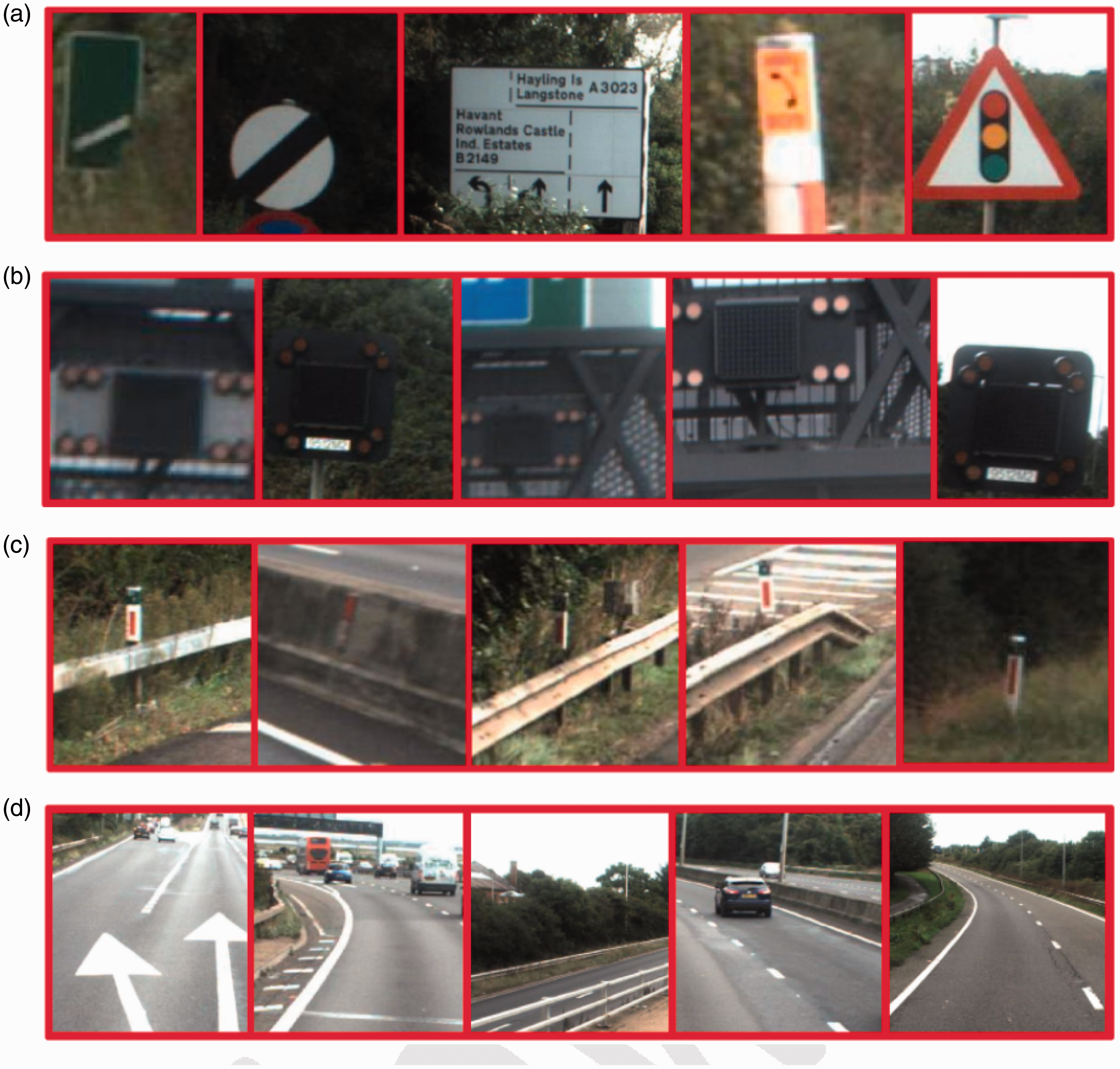
Examples of the training dataset for each class. Traffic signs, matrix signs, reference markers, and the empty (random images) class are shown in panels (a–d), respectively.

Table 2.
Number of Each Asset Type Used for Training and Validation of the Convolutional Neural Network (CNN), and to Test the Decision Support System

Asset type Train Validation Test

Traffic sign 800 200 149

Reference marker 800 200 69

Matrix sign 800 200 18

Random 800 200 0

Total 3200 800 236

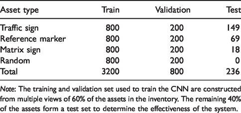
Note: The training and validation set used to train the CNN are constructed from multiple views of 60% of the assets in the inventory. The remaining 40% of the assets form a test set to determine the effectiveness of the system.

We chose the GoogleNet architecture, trained on roughly 1.2 million images from 1,000 different classes ( 36 ), as the initial CNN to be re-trained. The network ranked first in the ILSVRC 2014 classification challenge ( 37 ), and is available in the Matlab deep learning toolbox. The original fully connected neural network is changed so that the final classification layer has four nodes, and is therefore suitable for asset classification. The CNN is re-trained for 20 epochs, with a batch size of 32 and a learning rate of $1 \times 10^{- 4}$ . A classification accuracy of 98% is achieved on the withheld validation set.

Rapid Asset Inventory Update

We now test the method by considering those assets in the test set that are verified, and those identified for further manual inspection. Each asset is considered individually. First, the survey image for which the vehicle is closest to the asset and contains the asset’s bounding box is found. The asset is then cropped out of the image and classified by the CNN. For those assets classified as the asset type recorded in the inventory, we verify that the assets are recorded correctly in the inventory. Alternatively, assets that are classified as a different asset type than that recorded in the inventory, or as the empty class, are identified as assets that require further manual inspection. The inventory may be incorrect if the asset has been moved or removed from the highway, but the inventory has not been updated correspondingly, or the asset’s geographical or physical attributes are incorrect in the inventory. In addition, an asset is identified for further manual inspection if the view of the asset is impeded, or the CNN classifies the asset incorrectly. The system does not determine the reason for an incorrect classification. Rather, the relatively small number of assets for which this is the case are rapidly identified and presented to the analyst, who may then correspondingly update the inventory. Table 3 shows the number of assets that are verified and the reason for incorrect classification. Overall, 91% of highway-side assets in the test set are verified automatically. Examples of the system in operation are shown in Figure 5.

Table 3.
The Number of Assets that are Verified, and the Reason for an Incorrect Classification for Each Asset Type

Asset type Number Verified Percentage CNN error Impeded Incorrect inventory

Traffic sign 149 136 91 5 2 6

Reference markers 69 64 93 2 2 1

Matrix sign 18 15 83 2 0 1

Total 236 215 $91$ 9 4 8

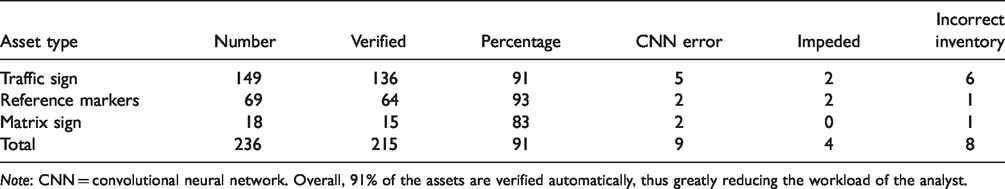
Note*: CNN = convolutional neural network. Overall, 91% of the assets are verified automatically, thus greatly reducing the workload of the analyst.

Figure 5.
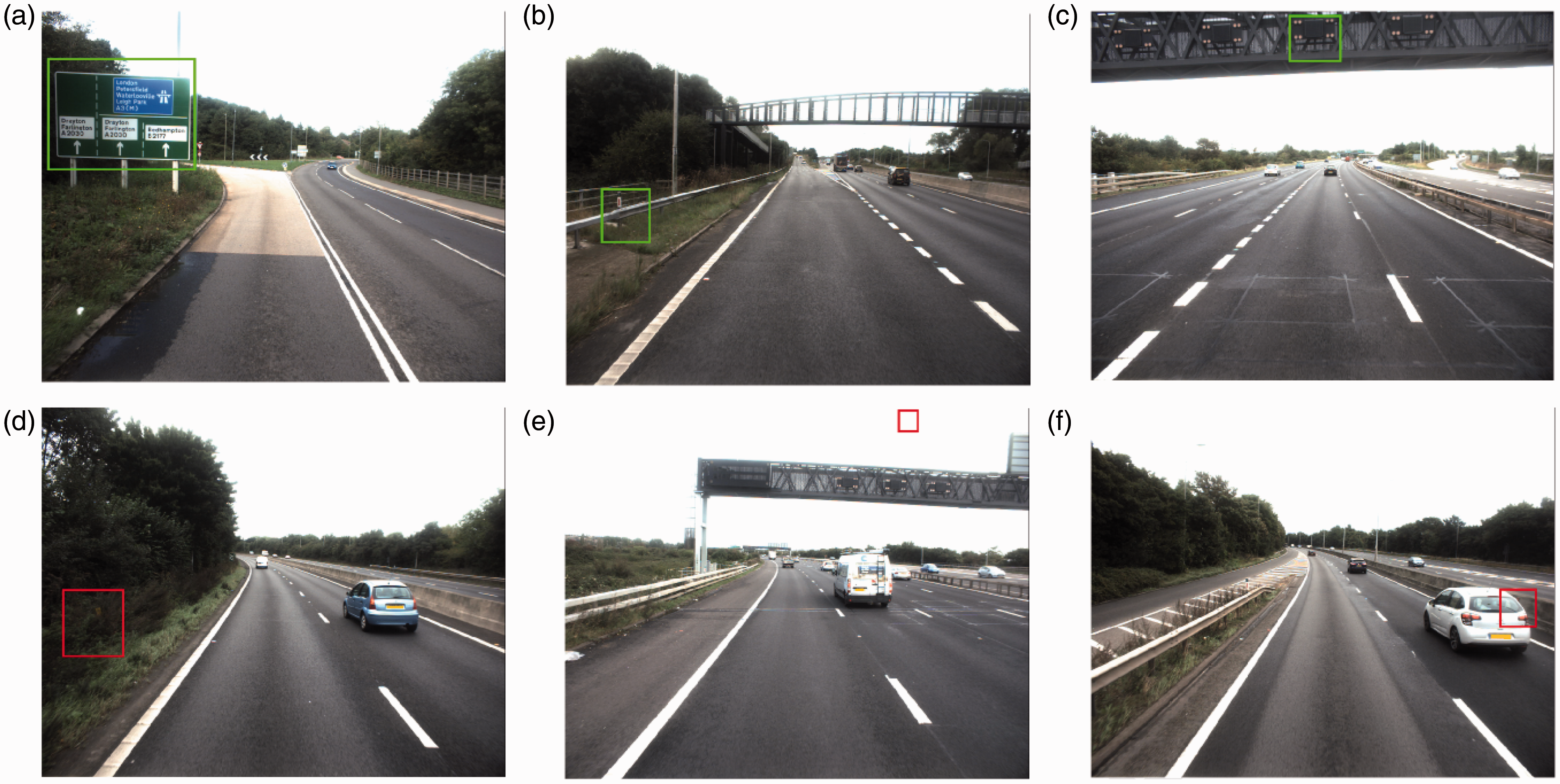
Six examples of the system in operation. Panels (a–c) show assets that are localized and classified as the correct asset type given in the inventory. Consequently, we automatically verify the inventory entry for those assets. Contrarily, assets that are classified as a different asset type in the inventory, or random, are shown in panels (d) and (e). A reference marker that has been moved without updating the inventory, and a matrix sign for which the mounting height is recorded incorrectly, are shown in panels (d) and (e), respectively. Panel (f) shows a reference marker for which the view is impeded by another vehicle.

Discussion

The system automatically verifies 91% of the assets in the withheld test set, which would otherwise be manually inspected by an analyst. The reduction in the number of assets that the analyst is required to manually inspect demonstrates the beginnings of a promising operational asset-monitoring capability. We do not consider whether the asset has been correctly verified. However, if an asset is correctly localized and classified by the CNN (which achieved a 98% classification accuracy), it is highly likely that the asset is recorded correctly in the inventory. The results show that the system performs well for all the asset types considered—although of the 21 assets identified for further manual inspection, 13 were the result of an incorrect classification by the CNN or an impeded view of the asset. However, going forward, we believe that training the CNN with a larger dataset and considering multiple images of the asset is likely to address these incorrect asset classifications.

There are several other potential refinements that might improve our method. Currently, three asset types have been considered; however, all roadside assets might be monitored by re-training the CNN with a labeled training dataset containing all asset types. Should the vehicle be equipped with a more sophisticated IMU, a more accurate heading direction might be computed, and thus, the heading correction would not be necessary. In addition, using a camera with known intrinsic parameters may simplify the camera calibration method, as only the six extrinsic camera parameters would be unknown. Furthermore, the camera parameters are assumed to be constant throughout the entire survey, and thus the camera is only calibrated once. However, it is possible that the camera angles might change should the vehicle jolt. Therefore, a sequential calibration method might be employed, so that the camera parameters are continually updated. Alternatively, auto-calibration methods such as those presented in Golparvar-Fard et al. ( 18 ) and Uslu et al. ( 19 ) might remove the need to manually collect control points.

Our system has several notable differences to existing TAM systems. Typically, assets (commonly traffic signs) are automatically detected in the images and subsequently processed ( 6 , 17 ). In contrast, our system employs a calibrated camera to project the assets (regardless of asset type) into the survey imagery, and thus our system is more robust (assuming an accurate calibration). On the other hand, along with several existing systems ( 15 , 16 ), we also exploit the efficacy of CNNs on image classification problems to perform asset classification.

Second, existing TAM systems consider primarily a data source from an external sensor (camera or LIDAR, for example) and subsequently detect and localize assets. However, our system is built on the inventory; that is, we firstly consider each asset as it is recorded in the inventory and subsequently verify its entry. Therefore, our method more accurately reflects the role of an analyst, and can thus provide rapid decision support within the current asset-monitoring process.

Conclusion

In this paper, a decision support system designed to assist those responsible for the maintenance of highway asset inventories is proposed. An inventory of assets along an 8 km section of the A27, data from a single forward-facing camera and a GPS-enabled IMU installed on a survey vehicle, and aerial imagery of the highway, was used to develop and test the system. By collecting control points, the camera was calibrated so that assets may be automatically localized within in-survey imagery, and a state-of-the-art CNN was re-trained to classify the assets. The inventory entry for an asset may then be verified if that asset is successfully localized and classified as the asset type recorded in the inventory—consequently the assets that require further manual inspection from the analyst are rapidly identified. The effectiveness of the system is determined by considering those assets in a withheld test set that are automatically verified, and those identified for further manual inspection. Overall, 91% of the assets are automatically verified, which would otherwise generate manual work. We have therefore proven the feasibility of the system, and its benefit to an analyst.

There are several limitations in the currently presented system, and therefore opportunities for further research and development. Currently, the system does not consider the asset condition, which is typically recorded in the inventory. Therefore, to further assist the analyst, future research should consider automatic evaluation of the asset condition. Furthermore, the system only considers assets on the highway that are in the inventory (correctly or incorrectly). Therefore, the system might also be extended to automatically identify assets that are not in the inventory at all; assets that have recently been installed, for example. To achieve this, improving the CNN so that assets may be localized and classified from the whole scene of the highway, rather than from cropped asset thumbnails, is likely to be the way forward. Assets identified in the survey imagery may then be searched for in the inventory, and thus assets missing from the inventory might be identified.

In addition, the system relies on a GPS-enabled IMU installed on the survey vehicle and therefore may perform poorly in closed environments such as tunnels or urban areas. In this paper, we do not consider such environments and the system is assumed to be in operation on an open, multi-lane highway. Therefore, to make the system more robust, future work should also focus on fusing the IMU with a source that might provide an estimate of the vehicle’s position in closed environments. Such an estimate might be provided by a visual odometry-based method in which the relative camera motion is estimated purely from the survey imagery.

Camera parameter	Value	Bounds
Focal length f_u (pixels)	2058	[0,10000]
Focal length f_v (pixels)	2267	[0,10000]
Roll α (degrees)	–1.604	[–30,30]
Tilt β (degrees)	–5.004	[–30,30]
Pan γ (degrees)	–0.052	[–30,30]
Offset x₀ (m)	1.765	[–4,4]
Offset y₀ (m)	0.088	[–2,2]
Height h (m)	2.301	[0,10]

Asset type	Train	Validation	Test
Traffic sign	800	200	149
Reference marker	800	200	69
Matrix sign	800	200	18
Random	800	200	0
Total	3200	800	236

Asset type	Number	Verified	Percentage	CNN error	Impeded	Incorrect inventory
Traffic sign	149	136	91	5	2	6
Reference markers	69	64	93	2	2	1
Matrix sign	18	15	83	2	0	1
Total	236	215	$91$	9	4	8

Footnotes

Acknowledgments

The authors would like to acknowledge the data, support and funding from Jacobs, Highways England and the Engineering and Physical Sciences Research Council that have made the work presented in this paper possible.

Author Contributions

The authors confirm contribution to the paper as follows: study conception and design: T.S., R.E.W., R.L.; data collection: T.S., R.E.W., R.L.; analysis and interpretation of results: T.S., R.E.W., R.L.; draft manuscript preparation: T.S., R.E.W., R.L. All authors reviewed the results and approved the final version of the manuscript.

Declaration of Conflicting Interests

The author(s) declared no potential conflicts of interest with respect to the research, authorship, and/or publication of this article.

Funding

The author(s) disclosed receipt of the following financial support for the research, authorship, and/or publication of this article: This work was supported by a National Productivity Investment Fund (NPIF) (award number 2107418) with contribution from Jacobs.

References

Office of Road and Rail. Highways Monitor: Update on Highways England’s Capital Planning and Asset Management. TSO, 2017.

National Academies of Sciences, Engineering, and Medicine. Use of Transportation Asset Management Principles in State Highway Agencies. The National Academies Press, 2013.

European Commission. Common Framework for a European Life Cycle Based Asset Management Approach for Transport Infrastructure Networks , 2017. https://cordis.europa.eu/project/rcn/204966/factsheet/en. Accessed July 5, 2019.

American Association of State Highway and Transportation Officials. AASHTO Transportation Asset Management Guide: A Focus on Implementation. American Association of State Highway and Transportation Officials, 2011.

US Department of Transport. Common Q’s and A’s Pertaining to Transportation Asset Management, 2018. https://www.fhwa.dot.gov/asset/faq.cfm. Accessed June 6, 2019.

Balali

Ashouri Rad

Golparvar-Fard

Detection, Classification, and Mapping of U.S. Traffic Signs using Google Street View Images for Roadway Inventory Management. Visualization in Engineering, Vol. 3, No. 1, 2015, p. 15.

Hartley

Zisserman

Multiple View Geometry in Computer Vision. 2nd ed. Cambridge University Press, Cambridge, 2004.

Gonzalez

R. C.

Woods

R. E.

Digital Image Processing. 3rd ed. Prentice Hall, Upper Saddle River, NJ, 2008.

Prince

S. J. D.

Computer Vision: Models Learning and Inference. Cambridge University Press, Cambridge, 2012.

10.

Loce

R. P.

Bala

Trivedi

Computer Vision and Imaging in Intelligent Transportation Systems. 1st ed. Wiley-IEEE Press, Hoboken, N.J., 2017.

11.

Arnoul

Viala

Guerin

J. P.

and M. Mergy. Traffic Signs Localisation for Highways Inventory from a Video Camera on Board a Moving Collection Van. Proc., Conference on Intelligent Vehicles. Tokyo, Japan, 1996, pp. 141–146.

12.

Greenhalgh

Mirmehdi

Real-Time Detection and Recognition of Road Traffic Signs. IEEE Transactions on Intelligent Transportation Systems, Vol. 13, No. 4, 2012, pp. 1498–1506.

13.

Sermanet

LeCun

Traffic Sign Recognition with Multi-Scale Convolutional Networks. The 2011 International Joint Conference on Neural Networks, San Jose, CA, 2011, pp. 2809–2813.

14.

Cireşan

Meier

Masci

and J. Schmidhuber. Multi-column Deep Neural Network for Traffic Sign Classification. Neural Networks, Vol. 32, 2012, pp. 333–338.

15.

Zhu

Liang

Zhang

X. Huang, B. Huang, and S. Hu. Traffic-Sign Detection and Classification in the Wild. IEEE Conference on Computer Vision and Pattern Recognition (CVPR), Las Vegas, NV, 2016, pp. 2110–2118.

16.

Kryvinska

Poniszewska-Maranda

Gregus

An Approach towards Service System Building for Road Traffic Signs Detection and Recognition. Procedia Computer Science, Vol. 141, 2018, pp. 64–71.

17.

Wang

K. C.

Hou

Gong

Automated Road Sign Inventory System Based on Stereo Vision and Tracking. Computer-Aided Civil and Infrastructure Engineering, Vol. 25, No. 6, 2010, pp. 468–477.

18.

Golparvar-Fard

Balali

de la Garza

J. M.

Segmentation and Recognition of Highway Assets using Image-Based 3D Point Clouds and Semantic Texton Forests. Journal of Computing in Civil Engineering, Vol. 29, 2015, p. 04014023.

19.

Uslu

Golparvar-Fard

de la Garza

J. M.

Image-Based 3D Reconstruction and Recognition for Enhanced Highway Condition Assessment. Proc., Congress on Computing in Civil Engineering, Miami, FL, 2011, pp. 67–76.

20.

Sairam

Nagarajan

Ornitz

Development of Mobile Mapping System for 3D Road Asset Inventory.

Sensors, Vol. 16, No. 3, 2016, p. 367.

21.

Tsai

Y. J.

An Automated Sign Retroreflectivity Condition Evaluation Methodology using Mobile LIDAR and Computer Vision. Transportation Research Part C: Emerging Technologies, Vol. 63, 2016, pp. 96–113.

22.

Mcloughlin

Deegan

Mulvihill

C. Fitzgerald, and C. Markham. Mobile Mapping for the Automated Analysis of Road Signage and Delineation. IET Intelligent Transport Systems, Vol. 2, No. 1, 2008, pp. 61–73.

23.

Zhang

Wang

K. C. P.

E. Yang, X. Dai, Y. Peng, Y. Fei, Y. Liu, J. Q. Li, and C. Chen. Automated Pixel-level Pavement Crack Detection on 3D Asphalt Surfaces using a Deep-Learning Network. Computer-Aided Civil and Infrastructure Engineering, Vol. 32, No. 10, 2017, pp. 805–819.

24.

Gaist. Highwayview Roadscape Information has Changed Forever. 2017. https://www.gaist.co.uk/highwayview. Accessed June 17, 2019.

25.

Department for Transport. 200 Million Funding Boost for England’s Roads. 2017. https://www.gov.uk/government/news/200-million-funding-boost-for-englands-roads. Accessed June 17, 2019.

26.

Radopoulou

S.C.

Brilakis

Automated Detection of Multiple Pavement Defects. Journal of Computing in Civil Engineering, Vol. 31, No. 2, 2017, p. 04016057.

27.

Highways England Asset Information Group. Asset Data Management Manual, Part 2 – Requirements and Additional Information. Highways England, 2019.

28.

Director General of the Ordnance Survey UK. A Brief Description of the National Grid and Reference System. His Majesty’s Stationery Office (HMSO), 1946.

29.

Goldstein

Classical Mechanics. 3rd ed. Addison-Wesley, Boston, MA, 2002.

30.

Sturm

Pinhole Camera Model. Springer U.S., Boston, MA, 2014, pp. 610–613.

31.

Zeiler

Fergus

Visualizing and Understanding Convolutional Networks.

European Conference on Computer Vision (ECCV), Vol. 8689, 2013, pp. 818–833.

32.

Krizhevsky

Sutskever

Hinton

G. E.

Imagenet Classification with Deep Convolutional Neural Networks. Proc., 25th International Conference on Neural Information Processing Systems, Lake Tahoe, Nevada, 2012, pp. 1097–1105.

33.

Simonyan

Zisserman

Very Deep Convolutional Networks for Large-Scale Image Recognition. International Conference on Learning Representations, San Diego, CA, 2015.

34.

Bottou

Large-Scale Machine Learning with Stochastic Gradient Descent. Proc., COMPSTAT’2010, Physica-Verlag HD, Heidelberg, 2010, pp. 177–186.

35.

Shin

H. C.

Roth

Gao

L. Lu, Z. Xu, I. Nogues, J. Yao, D. Mollura, and R. M. Summers. Deep Convolutional Neural Networks for Computer-aided Detection: CNN Architectures, Dataset Characteristics and Transfer Learning. IEEE Transactions on Medical Imaging, Vol. 35, 2016, pp. 1285–1298.

36.

Szegedy

Liu

Jia

P. Sermanet, S. Reed, D. Anguelov, D. Erhan, V. Vanhoucke, and A. Rabinovich. Going Deeper with Convolutions. IEEE Conference on Computer Vision and Pattern Recognition (CVPR), Boston, MA, 2015, pp. 1–9.

37.

Russakovsky

Deng

J. Krause, S. Satheesh, S. Ma, Z. Huang, A. Karpathy, A. Khosla, M. Bernstein, A. C. Berg, and L. Fei-Fei. Imagenet Large Scale Visual Recognition Challenge. International Journal of Computer Vision (IJCV), Vol. 115, No. 3, 2015, pp. 211–252.

Computer Vision for Rapid Updating of the Highway Asset Inventory

Abstract

Literature Review

Data Sources

Asset Inventory

Aerial Imagery

Survey Vehicle

Data Pre-Processing

Coordinate Transformation

Heading Correction

Camera Calibration

Camera Model

Control Points

Implementation

Asset Identification

Asset Localization

Image Classification

Rapid Asset Inventory Update

Discussion

Conclusion

Footnotes

Acknowledgments

Author Contributions

Declaration of Conflicting Interests

Funding

References