Sage Journals: Discover world-class research

Abstract

Highway safety has attracted significant research interest in recent years, especially as innovative technologies such as connected and autonomous vehicles (CAVs) are fast becoming a reality. Identification and prediction of driving intention are fundamental for avoiding collisions as it can provide useful information to drivers and vehicles in their vicinity. However, the state-of-the-art in maneuver prediction requires the utilization of large labeled datasets, which demand a significant amount of processing and might hinder real-time applications. In this paper, an end-to-end machine learning model for predicting lane-change maneuvers from unlabeled data using a limited number of features is developed and presented. The model is built on a novel comprehensive dataset (i.e., highD) obtained from German highways with camera-equipped drones. Density-based clustering is used to identify lane-changing and lane-keeping maneuvers and a support vector machine (SVM) model is then trained to learn the boundaries of the clustered labels and automatically label the new raw data. The labeled data are then input to a long short-term memory (LSTM) model which is used to predict maneuver class. The classification results show that lane changes can efficiently be predicted in real-time, with an average detection time of at least 3 s with a small percentage of false alarms. The utilization of unlabeled data and vehicle characteristics as features increases the prospects of transferability of the approach and its practical application for highway safety.

Connected and autonomous vehicles (CAVs) are currently an emerging topic among transportation researchers and practitioners because of advancements in sensing and vehicle technologies, as well as the rapid development of powerful software modules. The most promising advantage of autonomous vehicles (AVs) is in relation to road safety, as the human element will be removed from the task of driving, and thus, many collisions and driving mistakes will be eradicated (1, 2). To ensure the safety of AV passengers and, in general, of traffic participants, an AV should sense its surroundings appropriately, plan its motion using the safest options, and move according to the plan based on the current measurements received by its sensors ( 3 ). Decision-making usually is part of the planning module of AVs and, more specifically, of maneuver planning, which includes motion prediction and risk assessment (4, 5). Therefore, the necessity for AVs to safely navigate through dense urban traffic, complex road infrastructure, and areas with inconsistent traffic dynamics, leads to the need for correct predictions with regards to the behavior of drivers in the vicinity of an AV.

In recent approaches, it has been noted that predicting trajectories of vehicles in the vicinity of an AV is computationally complex and, therefore, not suitable for real-time applications (6, 7). Furthermore, it has been recognized that a large amount of data is usually needed to “learn” vehicle maneuvers to be able to recognize them efficiently in real-world driving (8, 9). Nevertheless, the state-of-the-art in the prediction of vehicle behavior for AV applications utilizes data that are either disclosed from the car manufacturing companies, simulated, captured for a specific vehicle type, or limited in relation to size, which leads to limited transferability of their potential results ( 10 ).

This paper aims to extend the state-of-the-art by providing a data-driven approach for unsupervised labeling and the subsequent prediction of lane-changing maneuvers. The main contribution of this paper is the use of density-based clustering to distinguish between lane-changing and lane-keeping maneuvers for automatic labeling. The approach is envisioned to reduce the effort of manually labeling driving maneuvers, and additionally provides an efficient real-time sequence classification methodology to predict lane changing proactively. Toward this aim, highly disaggregated naturalistic driving data from the highD dataset are utilized ( 11 ). The dataset consists of more than 45,000 km of naturalistic driving behavior from 16.5 h of drone-captured video data. Initially, patterns in the data are found through density-based clustering, and the obtained clusters are used as an input for a real-time long-short term memory (LSTM) deep neural network to identify lane-changing maneuvers.

The paper is structured as follows: initially, the literature with regards to driving behavior prediction is reviewed, and the methodology of the current work is presented. This is followed by a description of the data and its pre-processing for the proposed algorithms. Finally, the results of the unsupervised labeling, as well as the real-time LSTM model, are presented and discussed, in order for conclusions to be drawn from the applications by researchers and practitioners.

Literature Review

Vehicle maneuvers are characterizations of a vehicle’s motion with regards to its position and speed attributes on the road ( 4 ). With regards to lateral vehicle control, lane keeping and lane changing are fundamental aspects of highway driving and are mutually exclusive ( 12 ). Lane keeping describes the task of driving within the current lane without any intention of leaving it, while lane changing requires inter-related decisions among drivers in a definite hierarchy, which are affected by the necessity and desirability of changing the lane in which a vehicle is moving ( 13 ). Lane changes can be discretionary or mandatory depending on how the driver perceives conditions on the current and target lanes, as well as environmental conditions that influence the decision to change lanes ( 14 ). During lane changing, usually, the speed of the subject vehicle increases, and disturbances in the adjacent lane might also be observed, for example, if the lane-changing maneuver is aggressive ( 15 ). To counteract these disturbances, and enable safe lane changing, drivers interacting for a lane change should be alert and attentive. However, this is not always the case: it has been indicated that turn indicators are used for 44% of performed lane changes ( 16 ).

Lane-changing prediction, like other driving behavior prediction tasks, can be formulated as a regression or a classification problem (17, 18). In a regression formulation, the objective is to predict position and speeds values to map vehicle motion on the road, while a classification problem formulation is concerned with discretizing vehicle states which enable faster real-time discrimination between vehicle behaviors. With regards to data utilized for predicting lane changing, usually geographic positioning system (GPS) traces, or vehicle sensor readings such as radars and cameras, act as features to lane-changing prediction algorithms (19 –21).

As far as methodological approaches are concerned, machine learning and data-driven approaches have gained popularity. Support vector machines (SVMs) showed good results when trained on a manually labeled dataset with features and lane positions, to classify lane keeping and lane changing ( 22 ). Furthermore, the situation of the highway (slower preceding vehicle and free adjacent lane), along with the lateral movement of the vehicle, have also been considered for the lane-change prediction ( 23 ). SVM, along with Bayesian filter, has also been used for lane-change prediction using lateral position and steering angle ( 24 ). Neural networks can be trained and used to predict the future positions of a lane-changing vehicle but only in certain discrete sections and not over the complete maneuver process ( 25 ). Morris et al. ( 21 ) used relevance vector machines (RVM) to differentiate between lane changing and lane keeping when trained on features extracted from the road environment, vehicle signals, and driver tracking. Lane departures can be predicted using deep learning methods like convolutional neural network (CNN), which were trained on features extracted from physiological signals such as electrocardiogram heart rate, respiration signals, and so forth, and rear side view images (26, 27).

Based on the above literature review, certain issues have been identified. Initially, for the training datasets to be easily transferrable and valid, there is a need for highly variable attributes. This fact also makes these models depend on the validity of the sensor measurements used to identify lane changing. Furthermore, an extensive collection of signals and dependence on the sensors might hinder the real-time applicability of the developed classifiers. Moreover, it is observed that limited, or simulated data are employed for training and testing the developed classifiers. More importantly, it is prominent that data is either manually labeled or extensive post-processing took place, usually based on extra information such as lane position for data to be labeled as lane-keeping or lane-changing instances. Consequently, there is a gap in the literature with regards to the utilization of large naturalistic driving datasets and automatic unsupervised labeling of data, which could accelerate inference and real-time applications. Therefore, this study aims to extend the state-of-the-art by using a two-step approach, where initially classes are identified through density-based clustering, and then a deep learning algorithm is utilized for real-time intention prediction on a large naturalistic driving dataset.

Methodology

This study uses a two-step prediction process from raw data observations: Initially, an unsupervised method is used for learning driving intentions in relation to lane keeping or lane changing, and the results are used for labeling the raw measurements. The labeled data then act as input for the prediction of lane driving intention using a deep learning model. The purpose is to develop a data-driven method, which is not concerned with manual labeling of data.

Trajectory data usually contains information on the position, velocity, acceleration, and lane position of a vehicle. A vehicle should belong to the “lane-changing” class if, during the recorded trajectory, a full lane-changing maneuver takes place. On the other hand, if the vehicle stays in the same lane, it will belong to the “lane-keeping” class. Figure 1 illustrates a lane-changing process to distinguish between the two classes. A vehicle is moving straight on the highway in a specific lane and then decides to change. At point B, the vehicle starts executing a lane-changing maneuver, which is described by its lateral movement. At point C, the lane-changing event occurs as the vehicle’s center crosses from one lane to the other, while at point D, the driver completes the lane-changing process and follows its lane. Therefore, the trajectory of the vehicle consists of two lane-keeping stages (AB and DE) and one lane-changing stage (BD). A lane change is fully executed if all points (i.e., B, C, and D) lie within the observed section of the highway.

Figure 1.

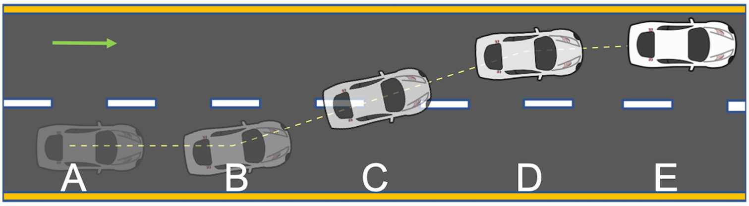
Illustration of lane-keeping (AB and DE) and lane-changing processes (BD) of a vehicle.

The lateral movement during lane changing is captured by lateral velocity and lateral acceleration time series. In this study, only lateral velocity and lateral acceleration are used as features. The position of the vehicle is not used because it is dependent on a particular reference frame and cannot be easily transformed over a large study area.

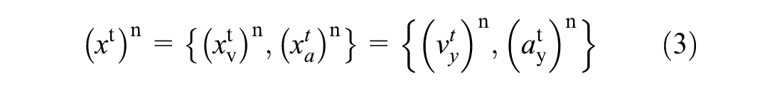
An outline of the proposed methodology is shown in Figure 2. The trajectory data consists of vehicle motion characteristics such as velocity and acceleration at each frame of video recording. Let the x-axis be along the longitudinal direction of the highway, and the y-axis be along the lateral direction (perpendicular to the highway). Let x denotes the set containing the lateral velocity and lateral acceleration measurements from trajectory data. Then, the value of x at time t for the nth vehicle is given by Equations 1, 2, and 3, where v_y and a_y represent velocity and acceleration along the lateral direction.

{(x_{v}^{t})}^{n} = {{(v_{y}^{t})}^{n}}

(1)

{(x_{a}^{t})}^{n} = {{(a_{y}^{t})}^{n}}

(2)

{(x^{t})}^{n} = {{(x_{v}^{t})}^{n}, {(x_{a}^{t})}^{n}} = {{(v_{y}^{t})}^{n}, {(a_{y}^{t})}^{n}}

(3)

Figure 2.

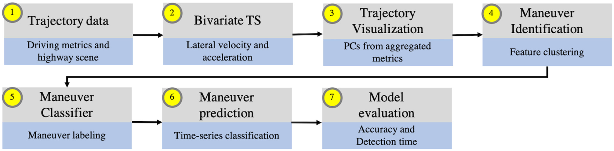
Flowchart of the proposed methodology.

Each x belongs to one of the two mutually exclusive classes, that is, lane keeping or lane changing. Thus, the primary objective is to classify trajectory measurements x into an appropriate maneuver class. We extract four features consisting of mean and standard deviation (µ₁,µ₂,σ₁,σ₂) from the bivariate time-series of lateral velocity and lateral acceleration for each vehicle (Equations 4 and 5). It is pointed out that other statistical features such as maximum, skewness, and kurtosis could also be potential candidates for subsequent analysis, depending on the characteristics of the driving behavior captured by the data. Then, a dimensionality reduction technique, principal component analysis (PCA) is used to obtain two principal components P₁ and P₂ from these features (Equation 6).

μ_{i}^{n} = \frac{1}{N^{n}} \sum_{t = t_{b}}^{t = t_{e}} {(x_{i}^{t})}^{n}, \forall i \in {v, a}

(4)

σ_{i}^{n} = \sqrt{\frac{1}{N^{n}} \sum_{t = t_{b}^{n}}^{t = t_{e}^{n}} {({(x_{i}^{t})}^{n} - μ_{i}^{n})}^{2}}

(5)

P_{1}^{n}, P_{2}^{n} = f (σ_{1}^{n}, σ_{2}^{n}, μ_{1}^{n}, μ_{2}^{n})

(6)

where

$N^{n} is the length of bivariate time series for vehicle n,$

$t_{b}^{n} is the time when the nth vehicle enters the frame of the video,$

$t_{e}^{n} is the time when the nth vehicle exits the frame of the video,$

$f (x) represents the principal component analysis .$

The two principal components are then plotted for ground truth to identify the two distinct classes of trajectories. These groups should represent mutually exclusive trajectories as far as lane changing is concerned, that is, the lane-changing class should include at least one lane-changing maneuver, and the lane-keeping class should contain no lane-changing maneuver. Furthermore, the first trajectory group (i.e., lane changers) can contain both lane-keeping and lane-changing maneuvers, but the lane-keeping group can only contain lane-keeping maneuvers.

For maneuver identification and prediction, it is necessary to recognize the motion within a trajectory and classify the segments of trajectory as either “lane-changing” or “lane-keeping.” This will be achieved by clustering the points from the bivariate time series (x^t)ⁿ by using the density-based spatial clustering of applications with noise (DBSCAN) algorithm. DBSCAN is effective in discovering clusters of arbitrary shapes with the least domain knowledge (28, 29). The tunable parameters for this type of clustering are the maximum distance for neighborhood point (eps), the minimum number of points to define a core point (minimum samples), and a metric for calculating distances. The points are randomly sampled from the selected trajectories to reduce the amount of computation load on the clustering algorithm. This forms the basis for our labeling of the time series into two classes. An SVM classifier is trained on the clustered labels to capture the distribution of the identified clusters, such that each (x^t)ⁿ can be assigned to one of the two maneuver classes (Equation 7). The main tunable parameters for SVM are the penalty parameter (C) and kernel function. The trained SVM classifier is used to label the time series into two maneuver classes.

{(M_{j}^{t})}^{n} = h ({(x^{t})}^{n}),

(7)

$where M_{j} is corresponding label {Lane Changing, Lane Keeping} \forall j {1, 2} obtained$

$from clustering$ , $h (x) represents the SVM classifier$

After obtaining the labeled data, a moving window time series classification for maneuver prediction will be employed with the use of an LSTM deep learning model. The following parameters affect the input for the time series classification:

Frame frequency, F is the frequency of data, for example, 25 Hz.

Frame granularity, f is the sampling rate of the time series data for using as an input for the model. If f = 2, this means the effective frame frequency is 12.5 Hz.

Prediction horizon time, p_t is the time in the future at which the prediction is being made.

Prediction horizon length, p is the time series steps corresponding to p_t and f. Thus, p = F*p_t/f

Lookback time, k_t is the past time (and corresponding data) used to make the prediction.

Lookback length, k is the time series steps corresponding to k_t and f. Thus, k = F*k_t/f

Discard Threshold, T is the length below which trajectories are not considered for training. Further T > p+k or T = p+k+b where b is the buffer length. The value of b = 10 for this study.

Only the vehicle trajectories, which showed at least one change, are selected from the dataset to account for class imbalance, since the majority of the trajectories do not execute lane-change. The time series for each vehicle is sampled at the rate of frame granularity, f, such that the time series for the n^th vehicle with corresponding labels is shown in Equation 8:

\begin{matrix} {[X, y]}^{n} = \\ [{(x^{t_{b}}, x^{t_{b} + f}, x^{t_{b} + 2 f} \dots x^{t_{b} + N - 2 f}, x^{t_{b} + N - f})}^{n}, {(M^{t_{b}}, M^{t_{b} + f}, M^{t_{b} + 2 f} \dots M^{t_{b} + N - 2 f}, M^{t_{b} + N - f})}^{n}] \end{matrix}

(8)

$where N = F * (t_{e} - t_{b} + 1)$

The short trajectories with length less than the discard threshold, T, are eliminated from the training dataset. The time-series data is transformed into rolling window data (Equation 9). In other words, the past time-series data of constant length is used to predict the class label at a future time step. The data is scaled to the range [0, 1] and split into training and validation data set so that vehicles in the training data are not included in the validation data.

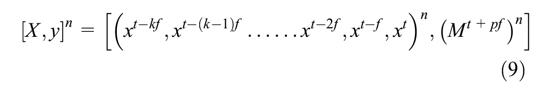
{[X, y]}^{n} = [{(x^{t - kf}, x^{t - (k - 1) f} \dots \dots x^{t - 2 f}, x^{t - f}, x^{t})}^{n}, {(M^{t + pf})}^{n}]

(9)

where t = αf, α is an integer, and f is the frame granularity

LSTM Networks

A special kind of neural network called recurrent neural networks (RNNs) consist of a chain-like structure consisting of multiple neural networks ( 30 ). This chain-like structure can be used for modeling temporal dependencies in a sequence. RNNs can model temporal dependencies well, but in practice, they face difficulties in modeling long dependencies (31, 32). LSTM is a special kind of RNN which is capable of learning long-term dependencies ( 33 ). LSTM has a similar chain-like structure but with modifications in the individual unit. LSTM consists of a memory cell and controls the flow of information by using input, forget, and output gate layers that discard the non-essential information and memorize only essential information for the purpose. LSTMs are successful in many tasks such as language translation, handwriting recognition, and image captioning (34 –36). They have also been applied to highway trajectory prediction and driver intention at intersections (17, 18). Random forests (RFs) are selected as a benchmark model for comparing the results with the LSTM model because of its simple tunable parameters yet robustness to variance in results ( 37 ). The main parameters for RF classifier are the number of estimators, maximum depth of the tree, and measurement criteria for the quality of the split.

Evaluation Criteria

The end-to-end detection model consists of multiple steps, such as clustering, labeling, and prediction. Thus, the performance of the complete model is dependent on the performance of these individual models. Clustering, label classification, and time-series classification-prediction are evaluated independently based on the common performance metrics for these algorithms. In addition to that, the performance of the complete model will also be evaluated using the classification evaluation metrics and advance detection time (ADT). These measures are discussed in the next paragraphs.

The ground truth labels for maneuver classification are not available, so the evaluation of the clusters is performed using one of the internal indices which measure the goodness of the clustering structure without external information (38, 39). One such internal index is the silhouette coefficient, with which each cluster is described by its silhouette based on the comparison of its separation and tightness ( 40 ). The silhouette coefficient is calculated using the mean intra-clustering distance and mean nearest-cluster distance for each sample. Silhouette score has a range of −1 to 1, with scores closer to 1 indicating good clustering performance. The classification algorithm is evaluated using the precision, recall, and accuracy scores (Equations 10, 11, and 12), and the LSTM training uses categorical cross-entropy loss (Equation 13).

Precision = \frac{TP}{TP + FP}

(10)

Recall = \frac{TP}{TP + FN}

(11)

Acuracy = \frac{TP + TN}{TP + TN + FP + FN}

(12)

where TP : True Positive, TN : True Negative, FP : False Positive, FN: False Negative

CE = - \sum_{i}^{M} M_{i} \log (s_{i})

(13)

where M_i and s_i are the ground truth and LSTM prediction for each maneuver class i in M.

The accuracy for LSTM is defined similarly to the classification accuracy defined above and is given by comparing the true value with the predicted value, and the percentage of correctly classified cases is reported as accuracy. The performance of the complete model is evaluated based on the correct classification and detection of the maneuvers in the trajectory. In addition to the aforementioned classification metrics, ADT is used to assess the predictive range of the model, as it shows how much in advance a prediction is made before a vehicle crosses the lane marking (i.e., point C in Figure 1). It should be noted here that ADT is different from the aforementioned prediction horizon time. The ADT depends on the performance of both the maneuver classification (SVM) as well as the prediction horizon time, p_t (LSTM).

Data Description

This study uses the highD trajectory dataset ( 11 ). The highD dataset is a naturalistic vehicle driving dataset collected on German highways using drone videography. The dataset consists of 60 recordings over 16.5 h from six locations (labeled 1–6) at a frame frequency of 25 Hz. The dataset covers four-lane (two per direction) and six-lane (three per direction) highways with central dividing median and hard shoulders on the outer edge. The dataset was recorded on highways with either no speed limit or with a limit of 120 km/h and 130 km/h. Recording of the data took place on weekdays between 08:00 and 19:00. The total distance driven by 110,000 vehicles (81% cars and 19% trucks) in the dataset is 45,000 km, with 5,600 complete lane changes ( 11 ). Krajewski et al. applied algorithms and post-processing to retrieve smooth position, velocities, and accelerations in both x and y directions ( 11 ). Besides, the dataset also contains the vehicle’s lane position and surrounding vehicles in each frame.

The current study uses only the lateral velocity and lateral acceleration time series from the dataset. The classification and prediction models are trained only on the trajectory data from recording no. 45 in location 1. The selected data contains 2,449 vehicles (2,034 cars and 415 trucks) recorded in 18 min, out of which 334 vehicles executed a lane change. The presence of cars and trucks in the dataset is useful for capturing driver behavior in mixed traffic. The configuration of the highway in this recording is six lanes. This data is split in 80:20 proportion for training and validation. The test data consists of 10,645 trajectories (6,128 trajectories with full lane change and 4,517 trajectories with no lane change), sampled from all the six locations in the dataset. In this study, trajectories are said to contain full lane-change if the lane-changing maneuver is between two lane-keeping maneuvers, as shown in Figure 1. This is the reason why the lane-changing trajectories in the test data are more than the full lane-change in the highD dataset, where lane-change is modeled using mathematical curves. This test data mostly represents free-flow traffic conditions, along with a few instances of the congestion in recording no. 12, 25, and 26. The congestion is used to refer to the traffic state when average lane speed is less than 75 km/h, which shows a speed drop when compared with the speed limit.

Results

The principal components obtained from the aggregate trajectory metrics, that is, µ₁,µ₂,σ₁,σ₂ explain 98% of the variance in the data. The principal component P₁ explains up to 94% of the variance. The scatter plot of the trajectories with P₁ and P₂ as axes show the two separate clusters of trajectories (Figure 3). This shows that lateral velocity and lateral acceleration are useful to distinguish between lane changing and no lane changing.

Figure 3.

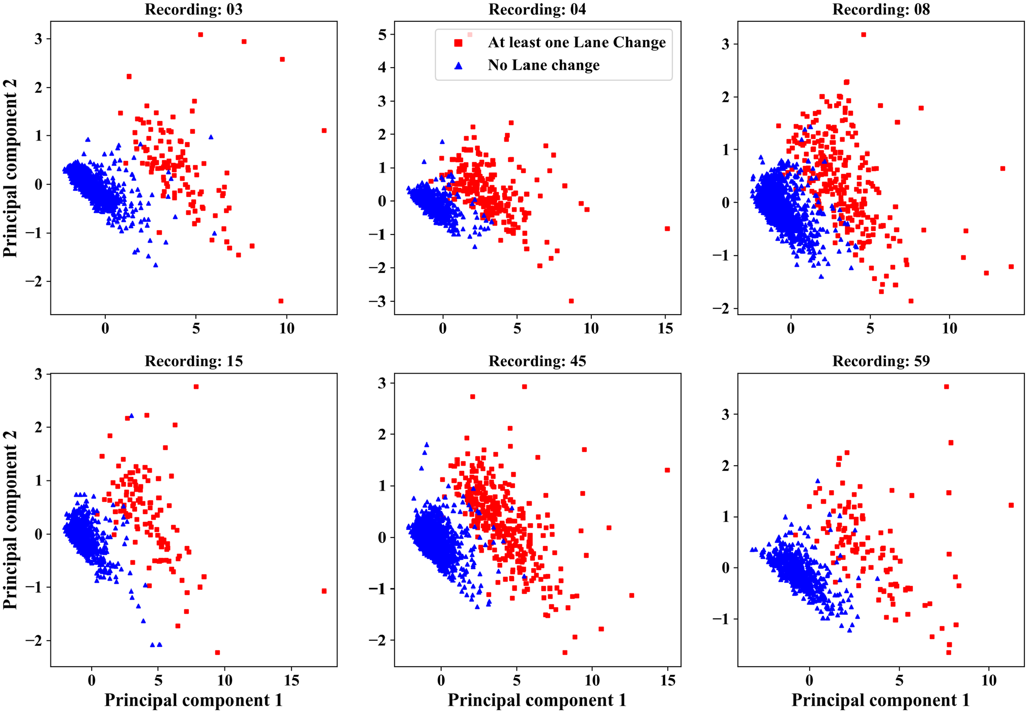
Principal components of features derived from lateral velocity and acceleration for different recordings (blue: vehicle trajectories without any lane change; red: trajectories which executed at least one lane change).

Figure 4 shows the result of the density-based clustering of the maneuvers. The parameters for clustering are eps = 0.05 and minimum samples = 80 with the Euclidean metric for distance calculation. These parameters are obtained by tuning the clustering for the Silhouette score. The Silhouette score for the two identified clusters corresponding to two maneuver classes is 0.74, which indicates good clustering performance. Each point in this scatter plot corresponds to the lateral acceleration and lateral velocity of a vehicle at one frame instance. The distribution plot of transverse acceleration and transverse velocity for lane-keeping maneuver follows a unimodal distribution with a mean close to 0 and a narrow deviation. This is because of the reason that during lane keeping, there are small deviations from the intended path. The distribution of lane changing has a bimodal distribution with a wide deviation. This is because of the reason that a lane-changing maneuver involves a significant acceleration and velocity during the lateral movement. The two peaks in the velocity distribution for lane changing are because of the left- and right-side lane changes.

Figure 4.

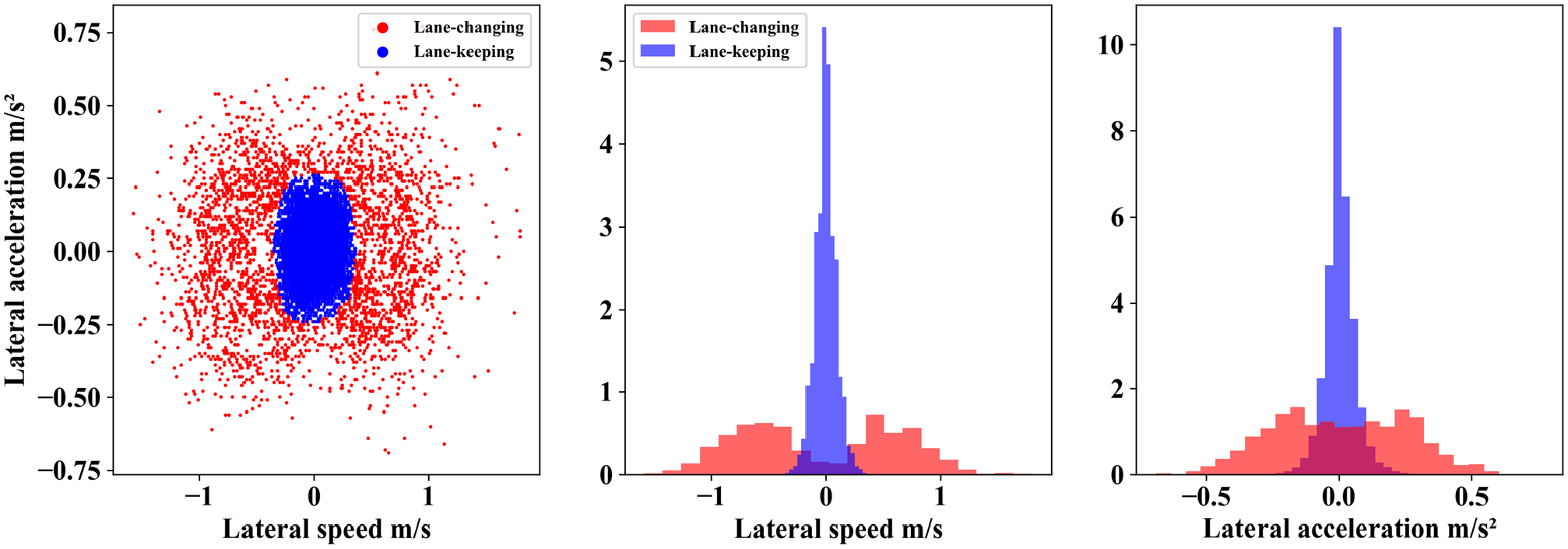
(Left) Maneuver clustering and (center) probability density plots of the lateral velocity and (right) lateral acceleration for the lane-changing and lane-keeping maneuvers.

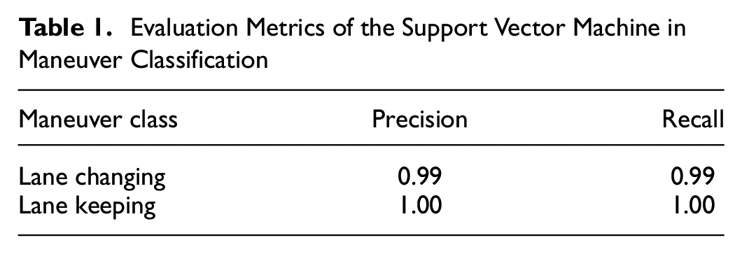
An SVM is trained on the clustered labels to learn the representations of the two maneuvers and thus label the bivariate time-series data during the inference stage. The best parameters for SVM are C = 0.5, with a radial basis function as a kernel. Table 1 shows the performance of the SVM maneuver classifier on the validation data. The maneuver classifier achieved an accuracy of 99.8% with high recall and precision, which shows the excellent performance of the SVM in distinguishing both classes. Based on the labeling, the duration of a full lane change is about 5.68 s, with a standard deviation of 0.77 s.

Table 1.

Evaluation Metrics of the Support Vector Machine in Maneuver Classification

Maneuver class	Precision	Recall
Lane changing	0.99	0.99
Lane keeping	1.00	1.00

The best configuration of the LSTM predictor is identified by its performance on the validation dataset and the training time. The selected model consists of two LSTM layers, each containing 50 units. The layers are stacked on top of each other to enable the model to learn higher-level temporal dependencies. The second LSTM layer returns its output to a dense layer with 20 neurons. A dense layer is a fully connected layer in which all the inputs are connected with all the outputs. This dense layer is further connected with two dense layers with 20 and 10 neurons. The final layer is also dense, but with softmax activation, and the output of the final layer is the probability of the two maneuver classes. Adam optimizer is used for adapting the learning rate ( 41 ). The training is stopped when validation accuracy does not improve over five consecutive iterations/epochs to avoid overfitting. The class with a higher probability score is the predicted class. Keras framework with TensorFlow as the backend is used for training the LSTM model (42, 43). The RF classifier is trained with the number of estimators = 10 and the maximum depth of the tree = 15. Gini impurity is used to measure the quality of the split.

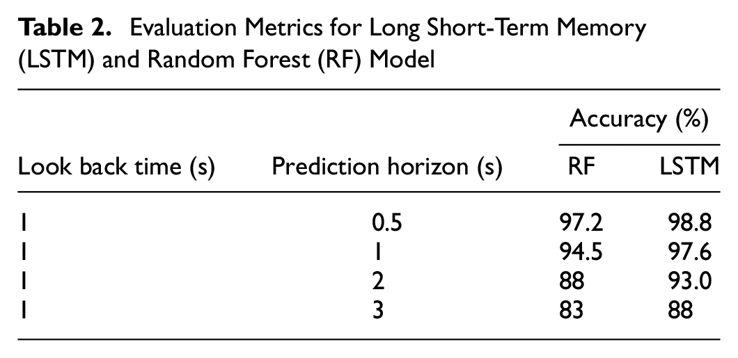
The lookback period greater than 1 s did not seem to have a significant improvement in the performance of the model. It was found that sampling the data with frame granularity, f > 1, results in longer training times, whereas training the model at the raw frame frequency, that is, f = 1, is faster and achieves the convergence much earlier. Thus, values of f = 1 and k_t = 1 s are used for the model training and evaluation. The loss and accuracy curves of the LSTM model for training data and validation data for different values of prediction horizon time p_t is shown in Figure 5. It can be seen that accuracy decreases with an increase in the prediction horizon since the dependencies are too long to be learned even by the LSTM model. Table 2 compares the results of maneuver prediction using the RF and LSTM models. At small prediction horizons, it can be seen that RF is as accurate as LSTM. However, when the prediction horizon increases, LSTM performs better than RFs. This is because LSTM is better designed to model the sequence or temporal dependencies. The LSTM model achieves an accuracy of above 97% for prediction horizon up to 1 s, which is very significant for highway driving scenarios. The accuracy drops significantly for prediction time greater than 1 s. As a result, the LSTM model, with a prediction horizon of 0.5 s, is used for the test data because of its high accuracy. Thus, the LSTM model can predict the lane-change maneuver 0.5 s before the start of maneuver with high accuracy.

Figure 5.

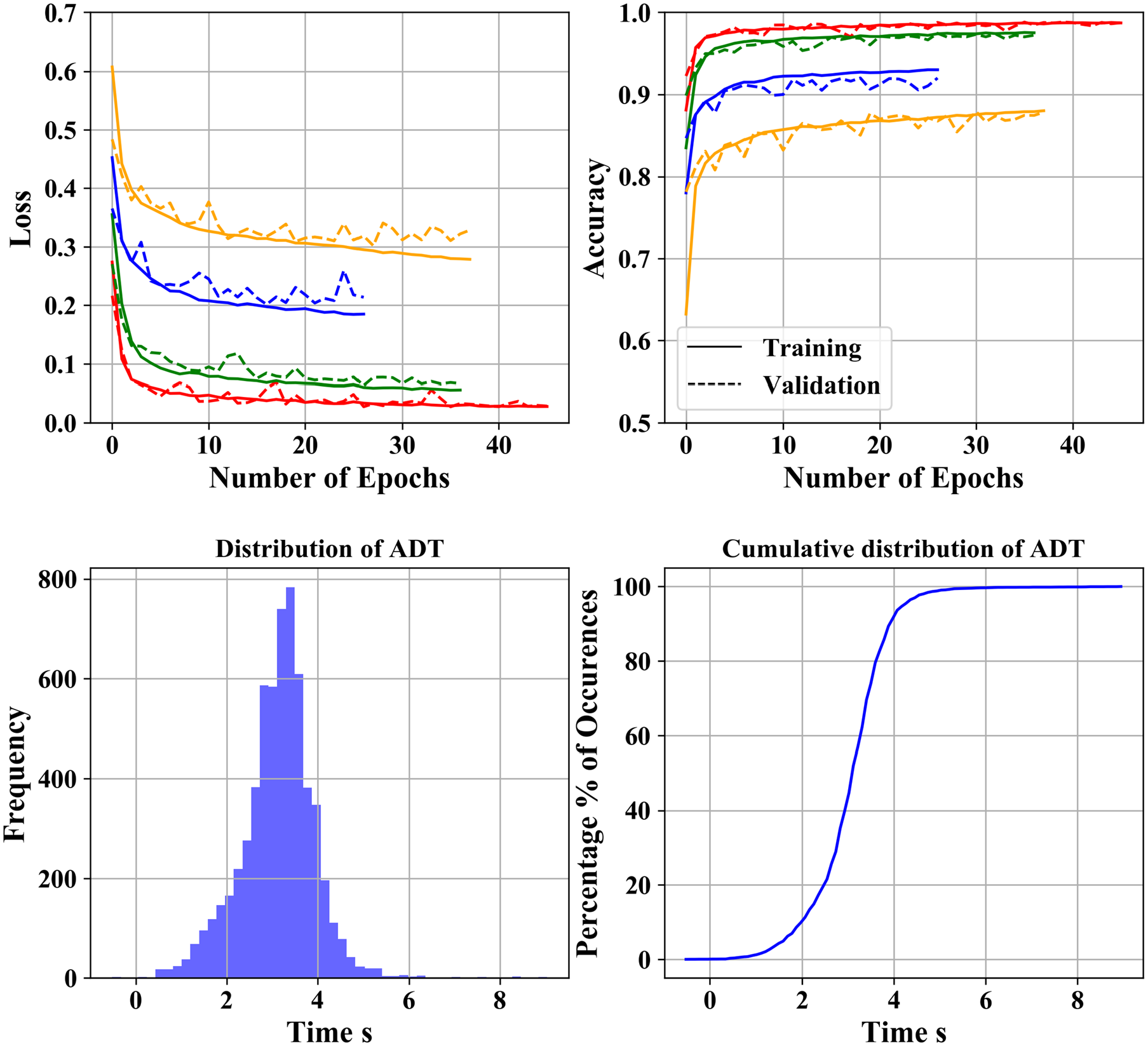
(Top) Loss and accuracy curves from the training and validation of the LSTM model for different prediction horizons, (bottom) Distribution and cumulative distribution of ADT.

Table 2.

Evaluation Metrics for Long Short-Term Memory (LSTM) and Random Forest (RF) Model

		Accuracy (%)
Look back time (s)	Prediction horizon (s)	RF	LSTM
1	0.5	97.2	98.8
1	1	94.5	97.6
1	2	88	93.0
1	3	83	88

The complete lane-change detection model is evaluated on the test data by using recall, precision, and ADT. The number of TP, FN, TN, and FP are 6,121, 7, 4,442, and 75, respectively. The model can detect the lane-change maneuver with a recall of 0.99 and a precision of 0.98 with a small percentage of false alarms (1.66%). The ADT has a mean of 3.18 s and a standard deviation of 0.98 s (Figure 5). This value is better than the detection time of 2.3 s obtained on simulation results and 1.3 s on real data (23, 24). The minimum, 90th percentile, 99th percentile, and maximum time for advance detection are −0.52 s, 4.04 s, 5.12 s, and 9.04 s, respectively. The negative minimum time corresponds to the case when the model detects the lane change 0.52 s after the vehicle crosses the lane marking.

A few examples of the maneuver prediction are shown in Figure 6. Here, the actual trajectory is color-coded as per the prediction and actual status of the maneuver. The initial length of trajectory is colored in black, since sufficient data is not available to make the predictions. The correct prediction for lane changing and lane keeping is shown by green and blue colors, respectively. It can be seen that the model performs accurately for different lane-change scenarios, such as left lane change, and right lane change. The few instances of misclassification of lane changing and lane keeping are shown in red and orange colors. Thus, the model can predict very well in advance before the vehicle crosses into an adjacent lane. The algorithm is expected to be reasonable for the CAV as shown by the ADT being more than the CAV’s reaction time, which is expected to be smaller than the human driver’s reaction time (0.4 s to 2.7 s) ( 44 ).

Figure 6.

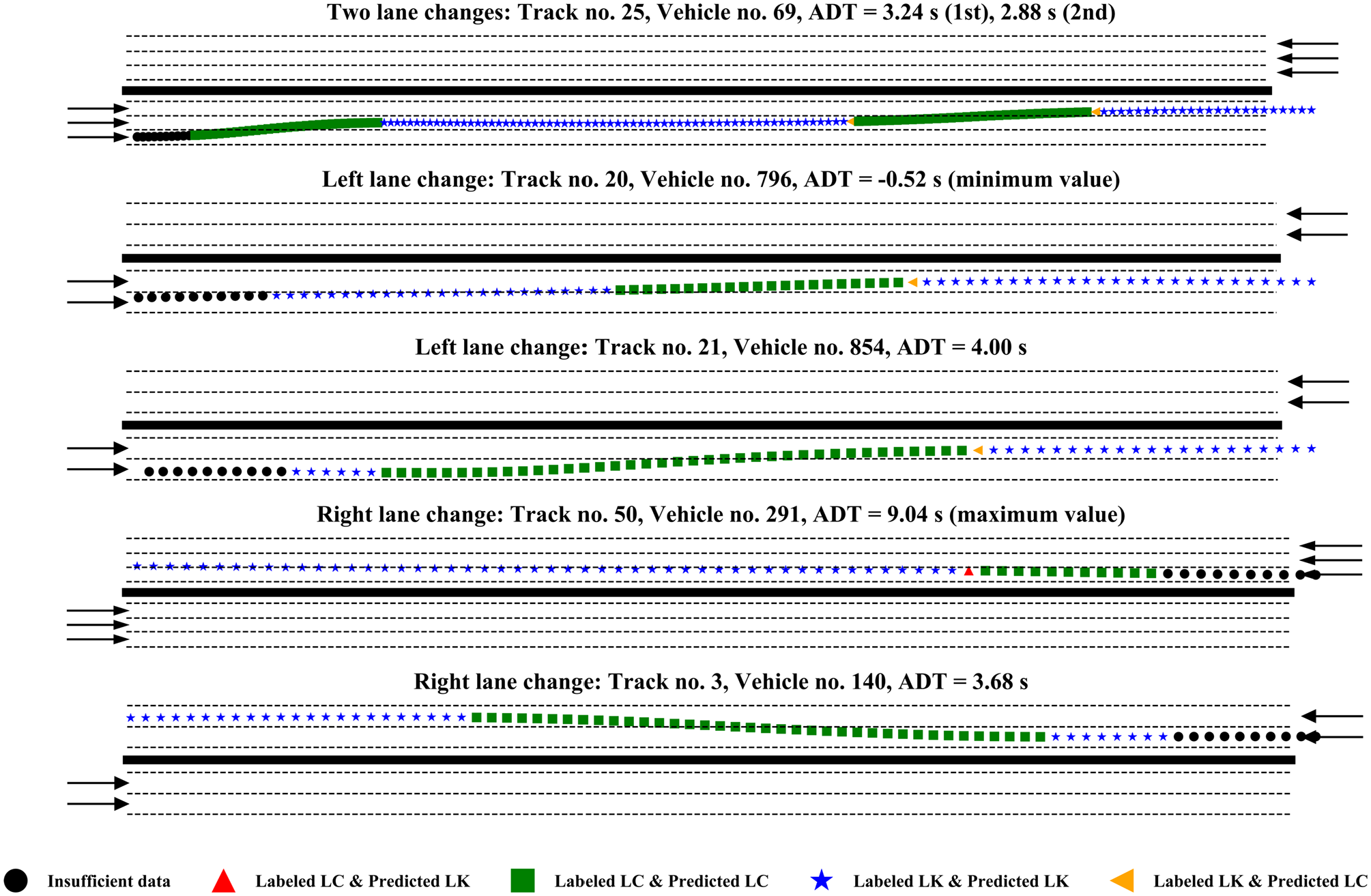
Examples of model predictions of the maneuver class for different trajectories. The maneuver prediction from LSTM at each point of the trajectory is compared with the labeled class. The blue star and green square indicate correct prediction for LK and LC, respectively.

Conclusion

Lane-changing and lane-keeping maneuvers are the two primary driving behaviors on highways. Their timely detection is one of the keys to highway safety and cooperative driving. However, data-driven prediction of these maneuvers has been so far constrained by data collection approaches and the manual labeling of training datasets. This study bridges the gap in the literature by demonstrating that only with lateral movement data in relation to velocity and acceleration it is possible to distinguish whether a vehicle will carry out a lane change or not. A density-based clustering approach and an SVM classifier demonstrated good results for automatically identifying and labeling maneuvers as lane keeping or lane changing. The unsupervised labeling approach is generic and can easily be transferred to other locations or scenarios for developing end-to-end maneuver detection models. Furthermore, the developed LSTM model for predicting maneuvers over trajectories from different highway locations shows a significant performance and can detect lane change at least 3 s before the vehicle crosses the lane markings.

The results of the study are envisioned to enhance highway safety, as successful and timely prediction can lead to better coordination among vehicles, and to proactive alerts to the drivers in the near and probably automated future. Furthermore, it is demonstrated that data from drones provide explicit information for extracting vehicle trajectories and should be further researched in the future, as suggested by previous studies ( 45 ).

Nevertheless, the presented research is not without limitations. The data recorded were obtained from a short highway segment, which consequently limits the number and nature of the identified maneuvers. Observing interactions over a longer road segment could help in observing more interactions. The data from radars, cameras, in-vehicle sensors, or automated traffic can also be used for validating the proposed lane-change detection method. Certain parts of methodology such as input pre-processing and model training will need to be adapted according to local data, and thus the future work will evaluate the application of the proposed methodology to different driving cultures or contexts. Finally, this study does not differentiate labels into the left or right lane change, and as a result, the utilization of the direction of the velocity to a frame of reference should be further researched.

Footnotes

Author Contributions

The authors confirm contribution to the paper as follows: study conception and design: V. Mahajan, C. Katrakazas, C, Antoniou; data collection: C. Katrakazas; analysis and interpretation of results: V. Mahajan; draft manuscript preparation: V. Mahajan, C. Katrakazas, C. Antoniou. All authors reviewed the results and approved the final version of the manuscript.

Declaration of Conflicting Interests

The author(s) declared no potential conflicts of interest with respect to the research, authorship, and/or publication of this article.

Funding

The author(s) received no financial support for the research, authorship, and/or publication of this article.

References

Virdi

Grzybowska

Waller

S. T.

Dixit

A Safety Assessment of Mixed Fleets with Connected and Autonomous Vehicles using the Surrogate Safety Assessment Module. Accident Analysis and Prevention, Vol. 131, 2019, pp. 95–111. https://doi.org/10.1016/j.aap.2019.06.001.

Campbell

Egerstedt

How

J. P.

Murray

R. M.

Autonomous Driving in Urban Environments: Approaches, Lessons and Challenges. Philosophical Transactions of the Royal Society A: Mathematical, Physical and Engineering Sciences, Vol. 368, No. 1928, 2010, pp. 4649–4672.

Katrakazas

Quddus

Chen

W. H.

A New Integrated Collision Risk Assessment Methodology for Autonomous Vehicles. Accident Analysis and Prevention, Vol. 127, 2019, pp. 61–79. https://doi.org/10.1016/j.aap.2019.01.029.

Katrakazas

Quddus

Chen

W. H.

Deka

Real-Time Motion Planning Methods for Autonomous on-Road Driving: State-of-the-Art and Future Research Directions. Transportation Research Part C: Emerging Technologies, Vol. 60, 2015, pp. 416–442. https://doi.org/10.1016/j.trc.2015.09.011.

Lefèvre

Vasquez

Laugier

A Survey on Motion Prediction and Risk Assessment for Intelligent Vehicles. ROBOMECH Journal, Vol. 1, No. 1, 2014, pp. 1–14.

Lefèvre

Laugier

Ibañez-Guzmán

Intention-Aware Risk Estimation for General Traffic Situations, and Application to Intersection Safety. INRIA Research Report No. 8379. INRIA, 2013.

Gindele

Brechtel

Dillmann

A Probabilistic Model for Estimating Driver Behaviors and Vehicle Trajectories in Traffic Environments. Proc., 13th International IEEE Conference on Intelligent Transportation Systems, Funchal, Madeira Island, Portugal, 2010, pp. 1625–1631. https://doi.org/10.1109/ITSC.2010.5625262.

Ziegler

Bender

Schreiber

Lategahn

Strauss

Stiller

Dang

Franke

Appenrodt

Keller

C. G.

Kaus

Herrtwich

R. G.

Rabe

Pfeiffer

Lindner

Stein

Erbs

Enzweiler

Knoppel

Hipp

Haueis

Trepte

Brenk

Tamke

Ghanaat

Braun

Joos

Fritz

Mock

Hein

Zeeb

Making Bertha Drive–An Autonomous Journey on a Historic Route. IEEE Intelligent Transportation Systems Magazine, Vol. 6, No. 2, 2014, pp. 8–20. https://doi.org/10.1109/MITS.2014.2306552.

Gindele

Brechtel

Dillmann

Learning Driver Behavior Models from Traffic Observations for Decision Making and Planning. IEEE Intelligent Transporation Systems Magazine, Vol. 7, No. 1, 2015, pp. 69–79.

10.

Ziegler

Bender

Dang

Stiller

Preliminaries

Trajectory Planning for BERTHA - A Local, Continuous Method. Proc., 2014 IEEE Intelligent Vehicles Symposium, Dearborn, MI, 2014.

11.

Krajewski

Bock

Kloeker

Eckstein

The HighD Dataset: A Drone Dataset of Naturalistic Vehicle Trajectories on German Highways for Validation of Highly Automated Driving Systems. Proc., 21st International Conference on Intelligent Transportation SystemsMaui, HI, 2018, pp. 2118–2125. https://doi.org/10.1109/ITSC.2018.8569552.

12.

Gayko

J. E.

Lane Departure and Lane Keeping. In Handbook of Intelligent Vehicles ( Eskandarian

, ed.), Springer, London, pp. 690–708.

13.

Gipps

P. G.

A Model for the Structure of Lane-Changing Decisions. Transportation Research Part B: Methodological, Vol. 20, No. 5, 1986, pp. 403–414. https://doi.org/10.1016/0191-2615(86)90012-3.

14.

Ahmed

K. I.

Modeling Drivers’ Acceleration and Lane Changing Behavior. PhD dissertation. Massachusetts Institute of Technology, 1999, p. 189.

15.

Ioannou

P. A.

Stefanovic

Evaluation of ACC Vehicles in Mixed Traffic: Lane Change Effects and Sensitivity Analysis. IEEE Transactions on Intelligent Transportation Systems, Vol. 6, No. 1, 2005, pp. 79–89. https://doi.org/10.1109/TITS.2005.844226.

16.

Lee

S. E.

Olsen

E. C. B.

Wierwille

W. W.

A Comprehensive Examination of Naturalistic Lane-Changes. No. DOT HS 809 702. National Highway Traffic Safety Administration, Washington, D.C., 2004.

17.

Zyner

Worrall

Ward

Nebot

Long Short Term Memory for Driver Intent Prediction. Proc., IEEE Intelligent Vehicles Symposium (IV), Los Angeles, Calif., 2017, pp. 1484–1489. https://doi.org/10.1109/IVS.2017.7995919.

18.

Altché

La Fortelle

A. D.

An LSTM Network for Highway Trajectory Prediction. Proc., 20th International Conference on Intelligent Transportation, Yokohama, Japan, 2018.

19.

Yang

Tang

Stewart

Dong

Zhang

Automatic Change Detection in Lane-Level Road Networks using GPS Trajectories. International Journal of Geographical Information Science, Vol. 32, No. 3, 2018, pp. 601–621. https://doi.org/10.1080/13658816.2017.1402913.

20.

Özgüner

Ü.

Stiller

Redmill

Systems for Safety and Autonomous Behavior in Cars: The DARPA Grand Challenge Experience. Proceedings of the IEEE, Vol. 95, No. 2, 2007, pp. 397–412. https://doi.org/10.1109/JPROC.2006.888394.

21.

Morris

Doshi

Trivedi

Lane Change Intent Prediction for Driver Assistance: On-Road Design and Evaluation. Proc., IEEE Intelligent Vehicles Symposium (IV), Baden-Baden, Germany, 2011, pp. 895–901. https://doi.org/10.1109/IVS.2011.5940538.

22.

Mandalia

H. M.

Salvucci

M. D.

Using Support Vector Machines for Lane-Change Detection. Proceedings of the Human Factors and Ergonomics Society Annual Meeting, Vol. 49, No. 22, 2005, 1965–1969.

23.

Wissing

Nattermann

Glander

K. H.

Hass

Bertram

Lane Change Prediction by Combining Movement and Situation Based Probabilities. IFAC-PapersOnLine, Vol. 50, No. 1, 2017, pp. 3554–3559. https://doi.org/10.1016/j.ifacol.2017.08.960.

24.

Kumar

Perrollaz

Lefèvre

Laugier

Learning-Based Approach for Online Lane Change Intention Prediction. Proc., IEEE Intelligent Vehicles Symposium, Gold Coast, Australia, 2013.

25.

Tomar

R. S.

Verma

Tomar

G. S.

Prediction of Lane Change Trajectories through Neural Network. Proc., International Conference on Computational Intelligence and Communication Networks, Bhopal, India, 2010, pp. 249–253. https://doi.org/10.1109/CICN.2010.59.

26.

Wang

Murphey

Y. L.

Kochhar

D. S.

MTS-DeepNet for Lane Change Prediction. Proc., International Joint Conference on Neural Networks, Vancouver, BC, 2016, pp. 4571–4578. https://doi.org/10.1109/IJCNN.2016.7727799.

27.

Jeong

S. G.

Kim

Min

End-to-End Learning of Image Based Lane-Change Decision. Proc., IEEE Intelligent Vehicles Symposium, Los Angeles, Calif., 2017, pp. 1602–1607. https://doi.org/10.1109/IVS.2017.7995938.

28.

Ester

Kriegel

H. P.

Jorg

A Density-Based Clustering Algorithms for Discovering Clusters. KDD-96 Proceedings, Vol. 96, No. 34, 1996, pp. 226–231. https://doi.org/10.1016/B978-044452701-1.00067-3.

29.

Schubert

Sander

Ester

Kriegel

H.-P.

DBSCAN Revisited, Revisited: Why and How You Should (Still) Use DBSCAN. ACM Transactions on Database Systems, Vol. 42, No. 3, 2017. https://doi.org/10.1145/3068335.

30.

Rumelhart

D. E.

Hinton

G. E.

Williams

R. J.

Learning Representations by Back-Propagating Errors. Nature, Vol. 323, 1986, pp. 533–536.

31.

Hochreiter

Untersuchungen Zu Dynamischen Neuronalen Netzen. Diploma thesis. Institut Für Informatik, Lehrstuhl Prof. Brauer, Technische Universität München. http://people.idsia.ch/~juergen/SeppHochreiter1991ThesisAdvisorSchmidhuber.pdf.

32.

Bengio

Simard

Frasconi

Learning Long-Term Dependencies with Gradient Descent Is Difficult. IEEE Transactions on Neural Networks, Vol. 5, No. 2, 1994, pp. 157–166.

33.

Hochreiter

Schmidhuber

Long Short-Term Memory. Neural Computation, Vol. 9, 1997, pp. 1735–1780.

34.

Sutskever

Vinyals

Q. V

. Sequence to Sequence Learning with Neural Networks. arXiv Preprint arXiv:1409.3215, 2014.

35.

Graves

Schmidhuber

Offline Handwriting Recognition with Multidimensional Recurrent Neural Networks. In Advances in Neural Information Processing Systems 21 ( Koller

Schuurmans

Bengio

Bottou

, eds.), Curran Associates, Inc., Red Hook, NY, pp. 545–552.

36.

Kiros

Salakhutdinov

Zemel

R. S.

Unifying Visual-Semantic Embeddings with Multimodal Neural Language Models. arXiv Preprint arXiv:1411.2539, 2014.

37.

Breiman

Random Forests. Machine Learning, Vol. 45, No. 1, 2001, pp. 5–32. https://doi.org/10.1023/A:1010933404324.

38.

Wang

Peng

CVAP: Validation for Cluster Analyses. Data Science Journal, Vol. 8, 2009, pp. 88–93. https://doi.org/http://doi.org/10.2481/dsj.007-020.

39.

Tseng

G. C.

Wong

W. H.

Tight Clustering: A Resampling-Based Approach for Identifying Stable and Tight Patterns in Data. Biometrics, Vol. 61, No. 1, 2005, pp. 10–16. https://doi.org/10.1111/j.0006-341X.2005.031032.x.

40.

Rousseeuw

P. J.

Silhouettes: A Graphical Aid to the Interpretation and Validation of Cluster Analysis. Journal of Computational and Applied Mathematics, Vol. 20, 1987, pp. 53–65. https://doi.org/https://doi.org/10.1016/0377-0427(87)90125-7.

41.

Kingma

D. P.

Adam: A Method for Stochastic Optimization. arXiv preprint arXiv:1412.6980, 2014, pp. 1–15.

42.

Chollet

Keras. https://keras.io/. Accessed July 30, 2019.

43.

Abadi

Agarwal

Barham

Brevdo

Chen

Citro

Corrado

G. S.

Davis

Dean

Devin

Ghemawat

Goodfellow

Harp

Irving

Isard

Jia

Jozefowicz

Kaiser

Kudlur

Levenberg

Mane

Monga

Moore

Murray

Olah

Schuster

Shlens

Steiner

Sutskever

Talwar

Tucker

Vanhoucke

Vasudevan

Viegas

Vinyals

Warden

Wattenberg

Wicke

Zheng

TensorFlow: Large-Scale Machine Learning on Heterogeneous Systems. arXiv preprint arXiv:1603.04467, 2015.

44.

Andréasson

Estimation of Driver Reaction Time from Car-Following Data: Application in Evaluation of General Motor–Type Model. Transportation Research Record: Journal of the Transportation Research Board, 2006. 1965: 130–141.

45.

Barmpounakis

E. N.

Vlahogianni

E. I.

Golias

J. C.

Babinec

How Accurate Are Small Drones for Measuring Microscopic Traffic Parameters?

Transportation Letters, Vol. 7867, 2017, pp. 1–9. https://doi.org/10.1080/19427867.2017.1354433.

Prediction of Lane-Changing Maneuvers with Automatic Labeling and Deep Learning

Abstract

Literature Review

Methodology

LSTM Networks

Evaluation Criteria

Data Description

Results

Conclusion

Footnotes

Author Contributions

Declaration of Conflicting Interests

Funding

References