Sensitivity Analysis to Define Guidelines for Predictive Control Design

Abstract

Signalized traffic control is important in traffic management to reduce congestion in urban areas. With recent technological developments, more data have become available to the controllers and advanced state estimation and prediction methods have been developed that use these data. To fully benefit from these techniques in the design of signalized traffic controllers, it is important to look at the quality of the estimated and predicted input quantities in relation to the performance of the controllers. Therefore, in this paper, a general framework for sensitivity analysis is proposed, to analyze the effect of erroneous input quantities on the performance of different types of signalized traffic control. The framework is illustrated for predictive control with different adaptivity levels. Experimental relations between the performance of the control system and the prediction horizon are obtained for perfect and erroneous predictions. The results show that prediction improves the performance of a signalized traffic controller, even in most of the cases with erroneous input data. Moreover, controllers with high adaptivity seem to outperform controllers with low adaptivity, under both perfect and erroneous predictions. The outcome of the sensitivity analysis contributes to understanding the relations between information quality and performance of signalized traffic control. In the design phase of a controller, this insight can be used to make choices on the length of the prediction horizon, the level of adaptivity of the controller, the representativeness of the objective of the control system, and the input quantities that need to be estimated and predicted the most accurately.

Signalized traffic control is important in traffic management to reduce congestion in urban regions. With recent technological developments, more data have become available to the controllers, varying from historical to real-time data, and from location-based data (like loop detectors) to floating-car data. Advanced state estimation and prediction methods have been developed that use these data ( 1 , 2 ). Some of these methods have already been applied in controllers to optimize traffic conditions proactively ( 3 , 4 ). To benefit fully from these techniques in signalized traffic controllers, it is important to look at the quality of the estimated and predicted input quantities in relation to the performance of the controllers. For the development of estimation and prediction methods on the one hand, and the design of traffic controllers on the other, it is important to have insight into the extent to which the accuracy of estimation and prediction will affect the performance of the controller.

Therefore, in this paper, the sensitivity of signalized traffic control for erroneous input quantities is addressed. A general framework for sensitivity analysis is proposed, to analyze the effect of errors in the measured, estimated, and predicted input quantities on the performance of different types of signalized traffic control. The framework is applied to predictive control, to analyze to what extent a prediction increases the performance of the controller, considering that the prediction contains errors. The results of the sensitivity analysis framework are used to set up design guidelines for predictive control.

In this paper, the following section gives a problem description followed by a short discussion of the state of the art on traffic control and sensitivity to input quantities. Then the sensitivity analysis framework is outlined, and demonstrated for predictive control. The results of the sensitivity analysis are presented and translated into design guidelines, and the paper is concluded with directions for future research.

This paper is a follow-up of the authors’ earlier work ( 5 ). The presented sensitivity analysis framework is the same, however, the presented case on predictive control is extended by considering a much longer prediction horizon, comparing the sensitivity to different input quantities, and looking into the influence of the degrees of freedom of the predictive controller. This gives new insights into the sensitivity of predictive controllers for errors in input quantities. Moreover, the experimental results in this paper are translated into guidelines for the design of such controllers.

Problem Description

In Figure 1, the process of signalized traffic control is outlined in relation to control theory. The controller influences the traffic process by its control signal. The traffic process is evolving in time, based on the internal traffic relations and external disturbances (demand, route choices). The traffic process can be monitored in real time by sensors, resulting in observed quantities. The observed quantities can be used to estimate the actual state of the traffic system expressed in derived quantities (like queue lengths). Likewise, the observed quantities can also be used to estimate (and predict) the disturbances. Based on the estimated state of the traffic system and a prediction of the disturbances, the future state of the traffic system can be predicted. Information on historical, actual, and future traffic states (combined with information on disturbances) is used as input for the controller. Based on this information, the controller determines the control scheme that implicitly or explicitly optimizes the performance of the traffic system.

Figure 1.

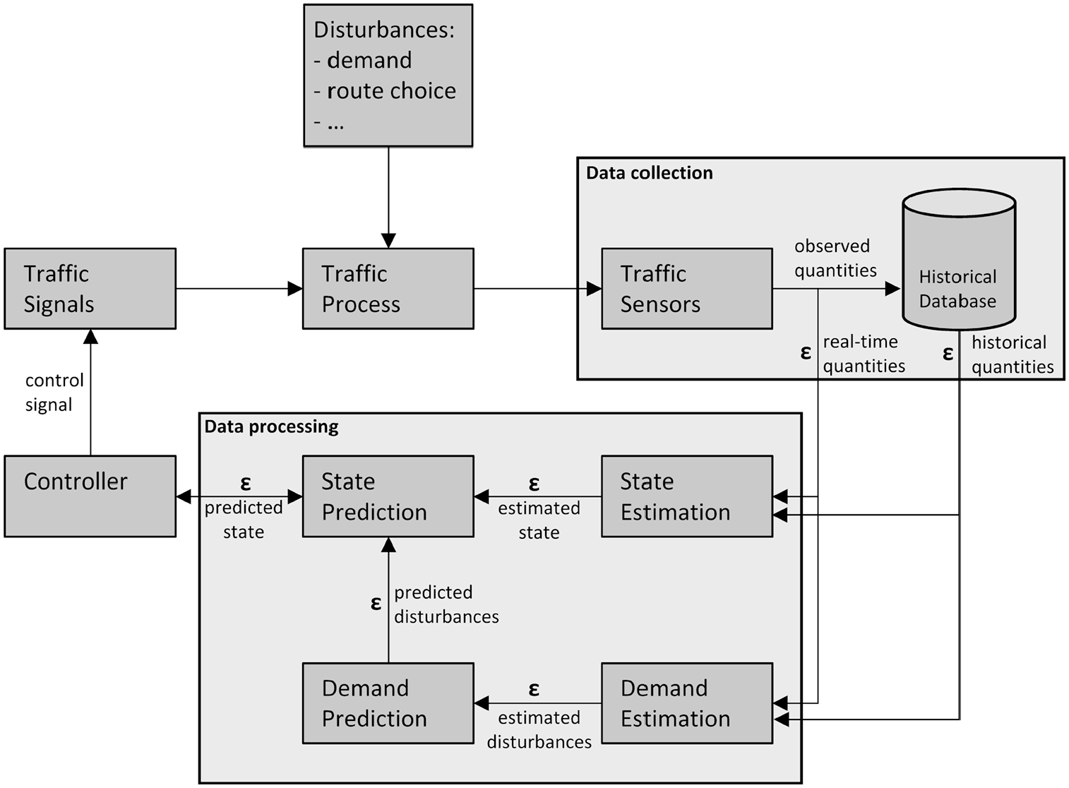
Process scheme of signalized traffic control with errors (ε) arising in the control process.

In this control process, errors may arise that can influence the control decision. In general, errors in the input quantities will eventually decrease the performance of the controller. Therefore, it is important to look at all elements in the control process where errors may occur. In monitoring the traffic system, an observation error will occur, caused by the inaccuracy of the sensor and observation method that is used. In the estimation of the traffic state (and disturbances) an estimation error is introduced, which may represent errors introduced by the estimation method itself or errors that were already present in the observed quantities. In the prediction of the traffic state (and disturbances), a prediction error is introduced. This error depends on the original error of the estimated state, and the prediction method. This prediction error will increase with the prediction horizon.

In the design of the controller as well as the estimation and prediction methods, it is important to know to what extent these errors influence the control decision and the performance of the controller. In this paper, this question is addressed by proposing a framework for sensitivity analysis on the observed, estimated, and predicted input quantities of signalized traffic control.

State of the Art

There is a wide variety of types of signalized traffic control ( 3 , 4 , 6 ). Signalized traffic control methods can be divided into two general categories: fixed-time control and traffic-responsive control. In fixed-time control, the control is optimized off-line, based on historical demand data. In traffic-responsive (or adaptive) control, the control is adapted in real time based on on-line data. The controller can react to the currently measured or estimated traffic situation, or it can proactively anticipate predicted traffic conditions. In general, the more detailed information is used, the more sensitive the controller performance is expected to be for errors in this information. Fixed-time control is quite robust for errors in the input quantities containing margins by design (implicitly in Webster-based cycle times, explicitly in robust control [ 7 ]). Traffic-responsive (or adaptive) control will be more sensitive to information errors, depending on the degrees of freedom of the controller.

Different levels of adaptive control can be distinguished by the degrees of freedom in the controller ( 3 ). In the first level, predefined control schemes are selected from a library based on the actual traffic conditions. In the second level, the control schemes are assumed to be cyclic, and cyclic parameters (like green splits) are adapted, based on information about the traffic conditions for current and upcoming cycles. In the third level, the control scheme is considered structure-free (no cycles). The combination and the order of movements can be adapted, together with the green times. In general, the more degrees of freedom there are in the controller, the better performance can be reached, the more sensitive the controller will likely be for errors in the estimated or predicted traffic conditions. In this paper this sensitivity will be analyzed for controllers with different degrees of freedom, varying from cyclic to structure-free control.

In the field of traffic management, sensitivity analysis on information errors has not yet received much attention. This holds not only for signalized control, but also for dynamic traffic management in general ( 8 ). The attention to this kind of analysis seems to have increased because of the introduction of floating-car data in the field of dynamic traffic management. For signalized control based on floating-car data, evaluating the influence of penetration rates and additional data errors is essential for a well-functioning system ( 9 ). With the increase of adaptivity of traffic controllers and the availability of more detailed information, the need for these sensitivity analyses on information errors is still increasing. This paper contributes to research on this issue.

Experimental Framework

In this section, a general framework for sensitivity analysis is proposed to analyze the effect of errors in the measured, estimated, and predicted input quantities on the performance of different types of signalized traffic control. Assuming perfect information, the ideal situation for a signalized traffic controller is created. Perfect information can be perfectly observed historical or real-time data, a perfect state estimation, or perfect prediction (no errors). Using a Monte Carlo approach, the perfect information is randomly disturbed, and the degeneration in performance of the controller is evaluated. The outcome of the sensitivity analysis will be an experimental relation between the level of information quality and the performance of signalized traffic control in the traffic system. The experimental framework is outlined in Figure 2.

Figure 2.

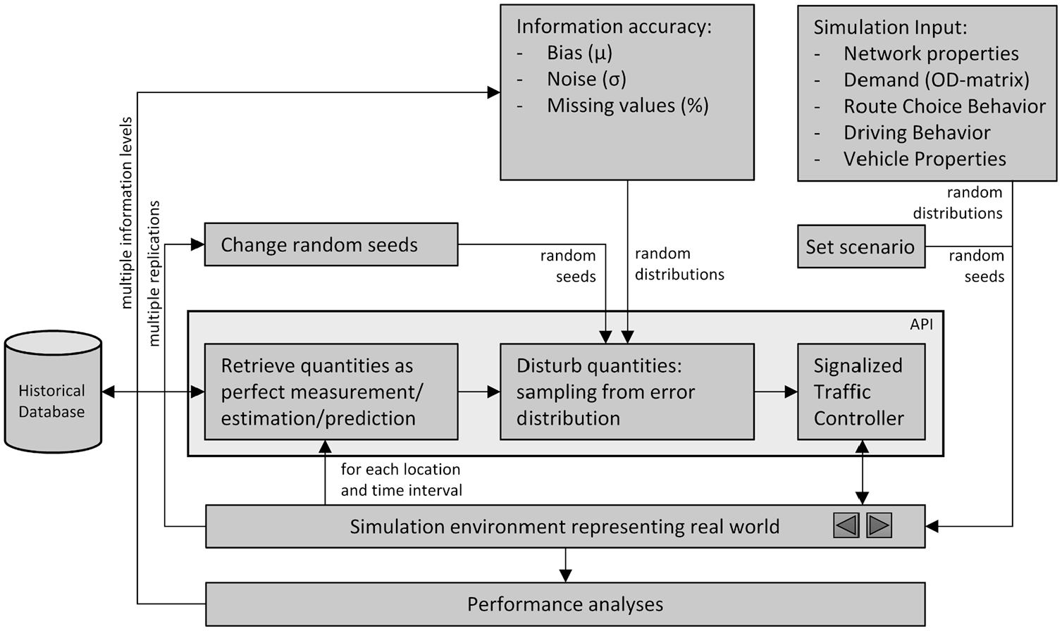
Experimental framework.

The framework makes use of a simulation environment to represent the real world. In an additional Application Programming Interface (API) the controller of interest is interacting with the simulation environment. A network configuration and a relevant demand scenario is chosen. Since the main goal of the sensitivity analysis is to determine the effect of errors in the input quantities of a controller and not to determine the effects of fluctuations in demand, the realization of the demand pattern is fixed during the sensitivity analysis. However, the sensitivity analysis can be repeated for different demand patterns (and network configurations) to compare the sensitivity to control input errors in different traffic conditions.

The main input to the sensitivity analysis is the information quality of the input quantities for the traffic controller. Information quality may consist of many aspects. In this framework, information accuracy of the input quantities is considered, expressed in a structural bias, a random noise, and a percentage of missing data, described by a random error distribution (of a properly chosen form). It is assumed that the information accuracy depends only on the observation, estimation, or prediction method, and does not depend on location and time, resulting in the same error distribution for each location and time. The realizations of the errors, however, differ over locations and time instances, and are independently drawn from the distributions. The effect of the errors can be simulated as follows:

• 0. Initialize the input error to no bias, no noise, no missing data (no error distribution yet) and simulate the situation with perfect information for the scenario. In this way, the ideal performance for the traffic controller is measured and set as a reference.

• 1. Increase the error by increasing the bias, noise, or percentage of missing vehicles. Adapt the random distributions for the control input errors accordingly.

• 2. Simulate multiple realizations of the errors to level out random variations over different locations and times. For each realized error pattern, for each control interval:

•  - Retrieve for each location the perfect input quantities from the simulation.

•  - Disturb the input quantities by the random realization of the error.

•  - Determine the control scheme based on the disturbed input quantities.

• 3. Measure the performance (note that it is assumed that the performance is measured perfectly in the simulation) and average over the simulated error realizations. Repeat the process from 1.

The output of the sensitivity analysis will be an experimental relation between the error in the input quantities and the performance of signalized traffic control in the traffic system for a given scenario.

Case: Predictive Control

The sensitivity analysis framework is in principle suitable for all types of signalized traffic control. However, in this paper, the framework is applied to traffic-responsive control with a predictive component. The main goal of the sensitivity analysis is to analyze to what extent a prediction improves the performance of the controller, considering that the prediction contains errors. The influence of the prediction horizon is studied, assuming errors accumulate for longer horizons. Different predictive controllers are considered with increasing degrees of freedom, varying from cyclic to structure-free control, to investigate the relation between adaptivity and performance, especially under erroneous predictions. A comparison is made with non-predictive control as well. Assuming a very short prediction horizon, predictive control can be considered as non-predictive control, where the controller only reacts to the current traffic situation. This is equivalent to a (conventional) vehicle-actuated control where a movement is given a green signal when vehicles are present. Since control behavior may depend on the demand, different demand scenarios are considered, that is, undersaturated, saturated, and oversaturated conditions. The sensitivity analysis is limited to a single intersection.

In the sensitivity analysis, different relations are tested, all related to design aspects of a predictive controller. For the different demand scenarios, it is verified:

• - Whether prediction improves the performance of a controller when perfect information is available. The relationship between prediction horizon and performance will be analyzed, and the prediction horizon length is identified beyond which performance does not improve any more.

• - Whether prediction still improves the performance of a controller, when errors are present in the predicted input data.

• - Whether a controller with high degrees of freedom, having a high adaptivity to anticipate fluctuating traffic patterns, is also more sensitive to errors in the predicted input quantities.

• - Which input quantity of the controller is the most sensitive to errors and therefore the most important to estimate or predict accurately.

• - Whether there are any unforeseen effects that need consideration in the design of predictive control.

In the next sections, first the predictive control model is specified in detail. Subsequently, the experimental settings of the control scenario are explained, concerning the intersection configuration, demand scenarios, and type of predictive controllers, then the results of the sensitivity analysis are presented. Finally, the results are translated into design guidelines for predictive control.

Predictive Control Model

The sensitivity analysis framework is specified for a predictive controller for a single intersection. The basis of the framework is the micro-simulation model Aimsun (Version 8.2.0), representing the ideal world. On top of this simulation framework, a predictive controller is implemented (using API). Based on the intersection configuration, the combinations and the possible order of the movements are predefined. The free control parameters, that is, the green times of the movements, are optimized based on a prediction of the traffic conditions.

A rolling horizon approach is used. At each control interval, the control sequence is updated in real time considering a new planning horizon. The objective of the controller is to minimize the total delay over the upcoming planning horizon, based on the current state (queues) and a prediction of the upcoming demand (arrival pattern). In the ideal simulation world, assuming perfect knowledge of the upcoming traffic situation, the expected delay could be determined by playing the simulation fast-forward for each candidate controller. To save computation time, however, a simple store-and-forward model with vertical queueing is used as a prediction model. Note that in this simplified prediction model, the predicted arrivals are perfectly known beforehand (since a single intersection is considered, the arrivals do not depend on control decisions). In the simulation environment, the non-delayed arrivals are stored and considered as the perfect predicted arrival pattern. The current state (queues) is also perfectly known from the simulation environment. Only the predicted departures are approximated by estimating vehicle passages through green, based on the state of the candidate control scheme and an approximation of the saturation flow rate. The saturation flow rate is experimentally obtained by measuring the queue discharge in the simulation environment (considering equal vehicles with the same average driving behavior).

The predictive controller can be expressed as a discrete mathematical programming problem. To this end, define the discrete time index k with duration T (s). Let i denote the index of a movement. Define movement group with index j, as a group of non-conflicting movements that can have green at the same time, and let I(j) be the set of movements belonging to movement group j. Let J(j) be the set of possible movement group indexes that can follow movement group j. Introduce signal states $s_i\left(k\right)\in \{0\left(\mathrm{red}\right),1\left(\mathrm{green}\right)\}$ and movement group states $p_j\left(k\right)\in \{0\left(\mathrm{red}\right),1\left(\mathrm{green}\right)\},$ for all movements i, movement groups j, and time indexes k for the prediction horizon [k₀,k₀+K]. The states should satisfy a predefined combination and order of the movements, forming the constraints of the optimization problem:

• - Composition of movement groups is respected:

$$s_i\left(k\right)=p_j\left(k\right)\forall i\in I\left(j\right)$$

(1)

• - Exactly one movement group is active:

$$\sum _j{p}_j\left(k\right)=1\forall k$$

(2)

• - Order of the movement groups is respected:

$$p_{\tilde{j}}(k+1)=0\forall \tilde{j}\notin J\left(j\right)\forall j:p_j\left(k\right)=1$$

(3)

The objective of the controller is to find the constrained signal states $s_i\left(k\right)\in \{0,1\}\forall i\forall k$ , and corresponding movement group states $p_j\left(k\right)\in \{0,1\}\forall j\forall k$ , that minimize the total delay over the prediction horizon [k₀,k₀+K], that is,

$${\min }_{\left\{s_i\left(k\right)\right\}}\sum _i\sum _{k=k_0}^{k_0+K}{x}_i\left(k\right)*T$$

(4)

with queue x_i(k) (vehicles) per movement i defined as:

$$x_i\left(k\right)=x_i(k-1)+a_i\left(k\right)-d_i\left(k\right)\forall k\forall i$$

(5)

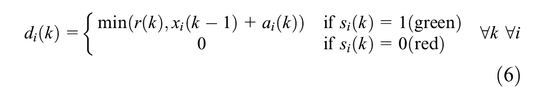
with arrivals a_i(k) (vehicles) and departures d_i(k) (vehicles) per movement i, where d_i(k) is approximated by an experimentally derived saturation flow curve r(k) (vehicles), that is,

$$d_i\left(k\right)=\{\begin{array}{cc}\min (r\left(k\right),x_i(k-1)+a_i\left(k\right))\hfill & \mathrm{if}{s}_i\left(k\right)=1(\mathrm{green})\hfill \\ \multicolumn{1}{c}{0}& \mathrm{if}{s}_i\left(k\right)=0(\mathrm{red})\hfill \end{array}\forall k\forall i$$

(6)

The discrete mathematical programming problem is solved following a branch-and-bound approach using decision trees. The pseudo code of the branch-and-bound process is given in Figure 3. Each node n in the decision tree is formed by the signal states s_i⁽ⁿ⁾(k) and corresponding movement group states p_j⁽ⁿ⁾(k) at time k, starting in the current state at the beginning of the planning horizon, k=k₀ (Initialization). The most promising node of the decision tree is selected to expand (Step 1). If the end of the planning horizon is reached, the sequence of movement groups is checked for its optimality (Step 2). While the end of the planning horizon is not yet reached, the node is branched to the next time interval of the planning horizon (Step 3). To this end, for each possible movement group transition, the new signal states are calculated (Step 3.1), and the queues and delay are updated (Step 3.2). Based on this new state information, it is decided if the new node is added to the search tree (branched) or is discarded (bounded). It is checked whether the state violates additional control constraints (Step 3.4), whether the state is already present in the decision tree with comparable or lower delay (Step 3.5), whether the delay is larger than the minimum delay so far (Step 3.6), if so, the node is discarded, otherwise, it is branched. Branched nodes are added to a search list (Step 3.8), from which the algorithm can continue the search process (Step 1).

Figure 3.

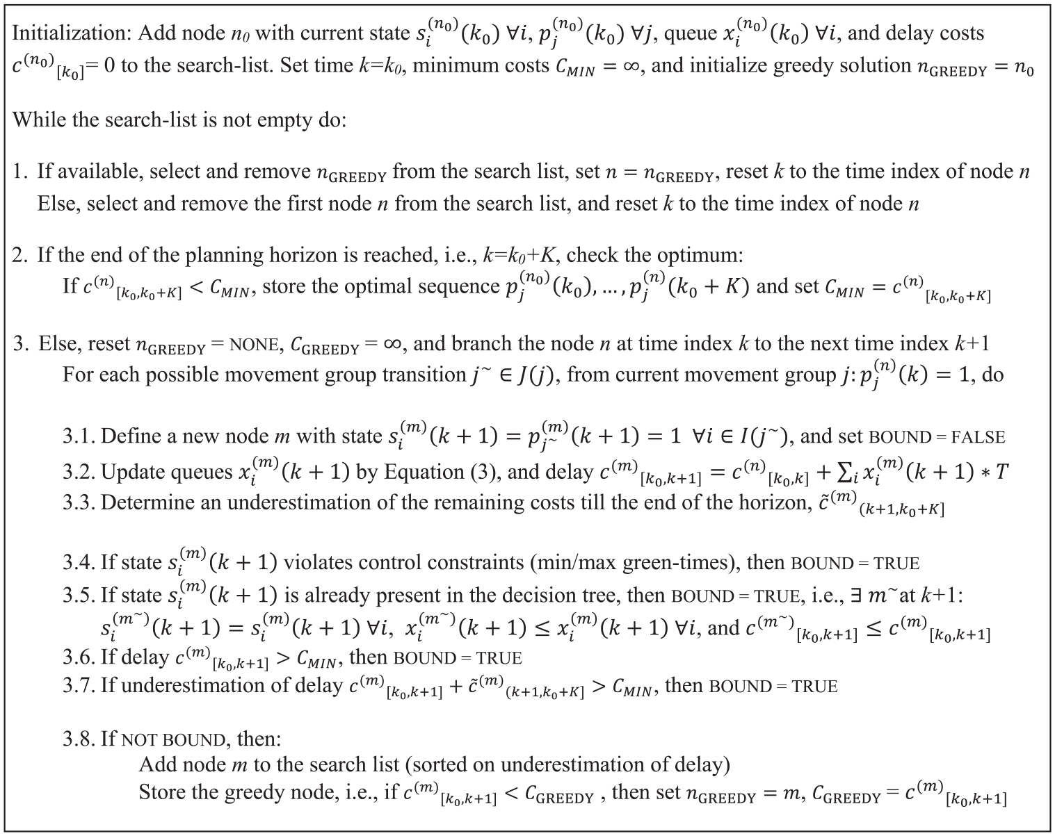
Pseudo code of branch-and-bound algorithm.

The depth of the decision tree is determined by the length of the prediction horizon, the width of the tree by the possible movement group transitions. The width of the decision tree can become quite large for increasing prediction horizons, especially if the set of movement group transitions J(j) is large. To be able to solve in real time, additional bound criteria are introduced that limit the size of the search space but still guarantee optimality. When the state and delay of a new node is updated, an underestimation of the entire delay to the end of the planning horizon is made (Step 3.3). This underestimation is used to check if the node can already be bounded (Step 3.7). Moreover, greedy initial solutions are used to speed up the search process. If a node is added (Step 3.8), and it has the minimum increase in delay in relation to the previous node, the node is chosen to be searched from in the next iteration (Step 1). This speeds up the algorithm considerably (and assures that there always is a (suboptimal) decision available, even if the algorithm is not ready yet).

The controller described so far uses perfect information. Now, however, in the sensitivity analysis, the input quantities are structurally disturbed and the mathematical programming problem is solved considering these erroneous input quantities and their influence on the delay of the control system is evaluated. The different input quantities, that is, predicted arrivals a_i(k), predicted departures (saturation flow) d_i(k), and current queue length x_i(k₀), are disturbed one by one, leaving the others untouched, to see which input quantity is most sensitive to errors. For this paper, it is assumed that the estimation or prediction method of the disturbed input quantity is biased (but no additional random noise is considered). For each input quantity a different independent structural error is introduced ${\mathrm{\epsilon }}_x,{\mathrm{\epsilon }}_a,{\mathrm{\epsilon }}_d\in (-1,\mathrm{\infty })$ for the queues x_i(k₀), arrivals a_i(k), and departures d_i(k), respectively. The disturbed quantities are defined by:

$${\tilde{x}}_i\left(k_0\right)=x_i\left(k_0\right)(1+{\mathrm{\epsilon }}_x)\forall i$$

(7)

$${\tilde{a}}_i\left(k\right)=a_i\left(k\right)(1+{\mathrm{\epsilon }}_a)\forall i\forall k$$

(8)

$${\tilde{d}}_i\left(k\right)=d_i\left(k\right)(1+{\mathrm{\epsilon }}_d)\forall i\forall k$$

(9)

Note that the considered quantities cannot have negative values. Therefore ${\mathrm{\epsilon }}_x,{\mathrm{\epsilon }}_a,{\mathrm{\epsilon }}_d$ should be considered in the range $(-1,\mathrm{\infty })$ . For errors ${\mathrm{\epsilon }}_x,{\mathrm{\epsilon }}_a,{\mathrm{\epsilon }}_d<0$ , the disturbed quantities become smaller than their original value, approaching 0 for errors approaching −1. For errors ${\mathrm{\epsilon }}_x,{\mathrm{\epsilon }}_a,{\mathrm{\epsilon }}_d>0$ , the disturbed quantities become larger than their original value. In this way, the error is varied in both directions, covering the whole possible range of values of the considered quantities. Further, note that the arrivals a_i(k) and departures d_i(k) are disturbed for the entire prediction horizon $\forall k\in$ [k₀,k₀+K]. The queue information is only disturbed for the current state k = k₀, and the queue values for the remaining horizon follow from Equation 5. Finally, note that the structural errors are equal for each time interval and movement. Since the introduction of relative errors may result in non-integer values, the disturbed quantities are rounded downwards to the nearest integer, and the remaining part is transferred to the next time interval or movement, to assure on average the specified error percentages.

Experimental Settings Control Scenario

The predictive control model is applied to a four-legged intersection with configuration as displayed in Figure 4a. The lanes are long enough, such that there is enough storage space for each direction and there is no spill-back to the network entrances. Three different demand scenarios are chosen, representing the undersaturated (almost no queues present), saturated (queues present but mostly solved after green phase), and oversaturated case (queues remain after green phase). The saturated case will probably be the most interesting, since errors in the input quantities of the controller can result in insufficient green times, resulting in a collapsing system with high delays. The undersaturated and oversaturated cases are chosen for the purposes of comparison, to see if the control is indeed most sensitive in saturated cases. The demand scenarios are simulated for 30 min (time-step 0.2 s). The arrivals are randomly distributed following an exponential arrival pattern with a constant mean (see Figure 4a for demand per movement). Each demand scenario is fixed to one repeatable realization.

Figure 4.

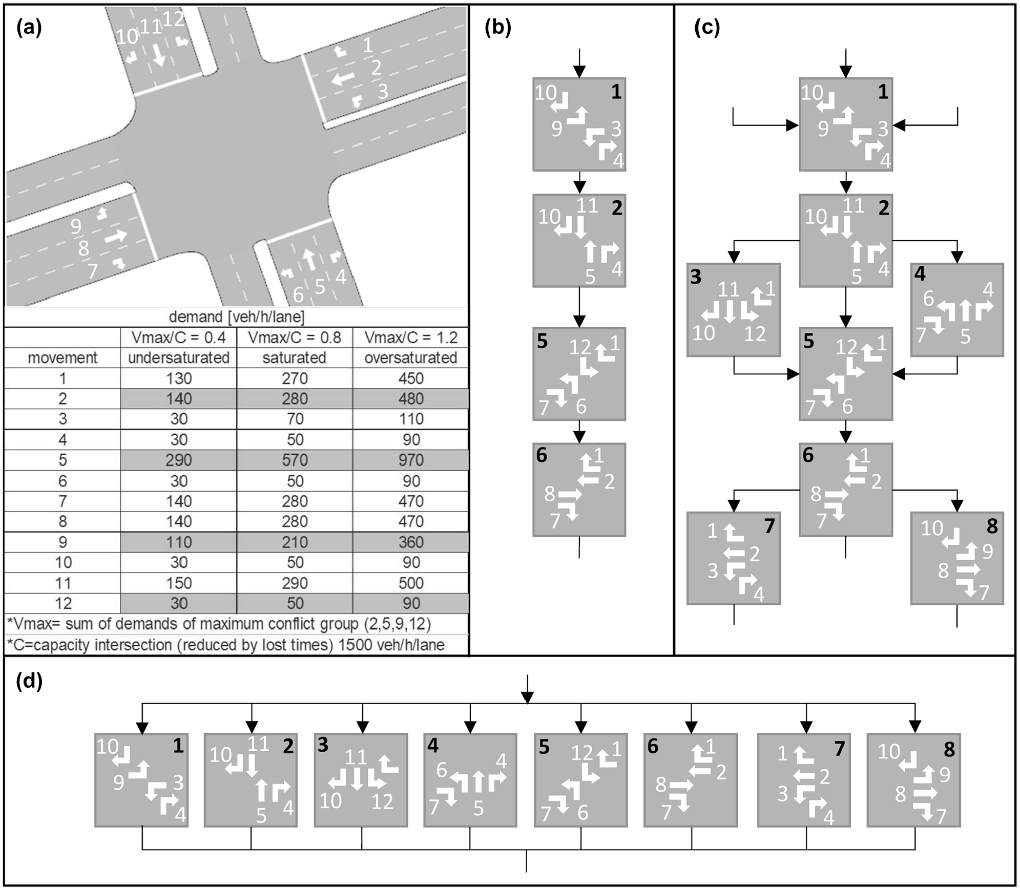
(a) Intersection configuration and demand scenarios, (b) cyclic control, (c) cyclic control with alternatives, and (d) structure-free control.

Different types of predictive controllers are considered, varying in the degrees of freedom in the controller. The controllers all use (a subset of) the same fixed predefined movement groups but vary in the set of possible movement group transitions (Equation 3). The basic structures of the controllers are depicted in Figure 4, b–d:

• - Cyclic control with four movement groups. The main movement groups (1, 2, 5, 6) are predefined and are only allowed in the cyclic predefined order. The cycle time differs per cycle resulting from the optimization process.

• - Cyclic control with alternatives, that is, four main movement groups and four additional movement groups. Next to the four main movement groups (1, 2, 5, 6), more flexibility is added to the predefined cycle by considering four additional movement groups (3, 4, 7, 8) that form an intermediate step between the main movement groups. The additional movement groups are optional, usage follows from the optimization process. The cycle time differs per cycle resulting from the optimization process.

• - Structure-free control with all eight movement groups. Main movement groups and additional movement groups are considered equal. There is a free choice in the order of all the eight movement groups. The order of the movement groups follows from the optimization process. No cycles are imposed anymore (although they can arise from the optimization process).

For all control types, additional constraints are applied on lost times (all-red time of 3 s), minimum green times (3 s), maximum green times (30 s for through and left movements and 60 s for right movements).

As outlined in the predictive control model, the controllers are based on a rolling horizon approach. Signal states (and the active movement group) can change each time interval (6 s). Each new control interval (12 s), the control sequence is updated in real time considering a new planning horizon. The planning horizon is varied from 0 to 120 s. In this case five short cycles of 24 s of the main movement groups with a minimum duration of 6 s each (3 s lost time + 3 s minimum green) can be evaluated, or one long cycle of 120 s of the main movement groups is possible with maximum green durations of 30 s (3 s lost time included). This gives the cyclic controllers the possibility to adapt to fluctuations in the arrival pattern. Note that a very short planning horizon (0 s) coincides with non-predictive control, where the controller only reacts to already arrived vehicles.

As explained in the section about the predictive control model, the arrivals are perfectly known beforehand, and can be fixed and stored in a preprocessing step for each demand scenario. The departures are approximated by experimentally derived saturation flow curves by measuring the queue discharge. The long-term saturation flow rate is one vehicle per 2 s. Using time intervals of 6 s, and an initial lost time of 3 s in the first interval, the discrete saturation flow curve is 1,2,2,3,3,3,3,… vehicles per time interval for increasing green duration. Using this preprocessed information, the controllers are all optimized on the fly, using the branch-and-bound solution method. The optimization problem is solved in real time, in 12 s, to come up with the new decision. In this time frame, exact solutions can be found for the cyclic controller and cyclic controller with alternatives for all planning horizons up to 120 s. For the structure-free controller, exact solutions can be found up to planning horizon of 60 s, after that, the computation time becomes too long, and therefore suboptimal solutions are used.

Experimental Results Sensitivity Analysis

Before the sensitivity analysis, as a reference, the performance of the control system is measured under perfect information. For the predictive controllers with increasing degrees of freedom (Figure 4), the performance of the system is analyzed for increasing prediction horizons. The results are presented in Figure 5 for the different demand scenarios. Note that the performance is expressed in delay per vehicle, obtained by dividing the total delay (objective) of the system by the number of vehicles, to get a more intuitive measure to compare the different demand scenarios. As Figure 5 shows, prediction improves the control system under perfect information. For all demand scenarios, the delay of the control system decreases for an increasing prediction horizon, and the performance is significantly better than for non-predictive control (considering a very short prediction horizon near zero). The structure-free controller with the highest degree of freedom achieves better performance in relation to delay and outperforms the cyclic controllers. There is a clear trade-off between adaptivity (degrees of freedom) and prediction horizon. The structure-free controller with high adaptivity can reach the same performance level with a short horizon, for which the cyclic controller with low adaptivity needs a much longer horizon. The gain of increasing the prediction horizon for the structure-free controller is less than for the more constrained cyclic controllers.

Figure 5.

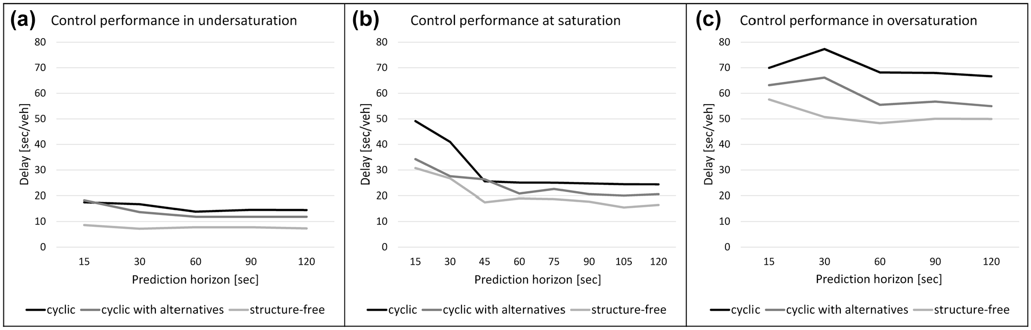
Performance of predictive controllers with perfect information on input quantities, for different demand scenarios: (a) undersaturated, (b) saturated, (c) oversaturated.

In general, there is a gain in performance by increasing the prediction horizon, although the gain in performance is less for longer horizons. For undersaturated conditions (Figure 5a), the line becomes flat from a certain prediction horizon. This point can be considered as the ideal prediction horizon length, that is, the best performance can be obtained using this prediction horizon, and (almost) no additional performance can be gained when looking further ahead in the future. For saturated conditions, there is no monotone decreasing behavior (Figure 5b). Since finite prediction horizons are used, a suboptimal control optimum is reached if actions in the control horizon influence the traffic condition after the end of the prediction horizon (especially the case in highly saturated conditions). For different horizon lengths, the suboptimal solution is suboptimal in a different way, resulting in fluctuating performance levels. The ideal prediction horizon is less obvious in such situations and is approximated visually. For each demand scenario, the performance with perfect data is set as a reference (indexed to 100 for the structure-free controller).

In the sensitivity analysis, the different input quantities, that is, predicted arrivals, predicted departures (saturation flow), and current queue state, are one by one structurally disturbed to see which input quantity of the controller is most sensitive to errors. For the disturbed quantity, the errors ${\mathrm{\epsilon }}_x,{\mathrm{\epsilon }}_a,{\mathrm{\epsilon }}_d$ (Equations 7–9) are taken from the set {−1, −0.5, −0.2, −0.1, 0, 0.1, 0.2, 0.5, 1}, and the performance of the controller is measured. Additionally, the relation between the performance and the horizon length is analyzed for the different error levels, and the ideal prediction horizon is determined to see if prediction still improves the performance of the system. In Table 1, this ideal prediction horizon and the performance are compared with the situation with perfect information. This is done for the different types of controllers, to see which controller is most sensitive, and for the different demand scenarios, to see if the results differ in undersaturated, saturated, and oversaturated conditions.

Table 1.

Overall Results of Sensitivity Analysis

		Undersaturated						Saturated						Oversaturated
		Cyclic		Cyclic withalternatives		Structure-free		Cyclic		Cyclic withalternatives		Structure-free		Cyclic		Cyclic withalternatives		Structure-free
Quantity	Error(%)	Delay(idx)*	Horizon(s)	Delay(idx)*	Horizon(s)	Delay(idx)*	Horizon(s)	Delay(idx)*	Horizon(s)	Delay(idx)*	Horizon(s)	Delay(idx)*	Horizon(s)	Delay(idx)*	Horizon(s)	Delay(idx)*	Horizon(s)	Delay(idx)*	Horizon(s)
Queue (state)	−100	288	60	198	60	121	30	193	90	163	90	159	90	168	90	160	90	144	90
	−50	225	60	165	60	100	30	162	60	131	90	125	60	144	60	115	60	103	90
	−20	193	60	165	60	100	30	152	60	126	60	108	60	139	60	114	60	100	60
	−10	193	60	165	60	100	30	148	60	125	60	101	60	139	60	114	60	100	60
	0	193	60	165	60	100	30	148	60	124	60	100	60	138	60	114	60	100	60
	10	193	60	165	60	100	30	148	60	126	60	101	60	139	60	114	60	100	60
	20	198	60	166	60	101	30	150	60	128	60	104	60	140	60	114	60	101	60
	50	226	60	168	60	104	30	156	90	140	60	121	90	145	60	115	60	109	60
	100	236	90	197	60	127	60	199	90	159	90	138	90	153	60	122	60	111	60
Arrival pattern	−100	258	0	259	0	309	0	195	90	186	90	191	60	154	60	127	60	117	60
	−50	255	30	208	0	152	0	153	90	146	90	119	60	138	60	114	60	100	60
	−20	204	60	167	60	123	30	148	60	131	60	104	60	138	60	114	60	100	60
	−10	196	60	165	60	104	30	148	60	128	60	101	60	138	60	114	60	100	60
	0	193	60	165	60	100	30	148	60	124	60	100	60	138	60	114	60	100	60
	10	216	60	165	60	100	30	152	60	126	60	104	60	138	60	115	60	101	60
	20	218	60	165	60	100	30	158	60	130	60	111	60	138	60	118	60	105	60
	50	221	60	168	60	100	30	183	90	140	90	131	90	141	90	130	90	115	90
	100	253	60	213	60	100	30	198	90	188	90	193	90	169	90	156	90	142	90
Departure pattern	−100	>400	30	>400	30	>400	60	>500	120	>500	90	>500	60	>300	90	>300	90	>300	90
	−50	268	30	223	30	148	60	236	120	213	90	228	60	162	90	156	90	149	90
	−20	217	60	188	60	113	30	174	90	138	90	155	60	145	60	129	60	113	60
	−10	212	60	167	60	111	30	158	60	131	60	135	60	142	60	122	60	105	60
	0	193	60	165	60	100	30	148	60	124	60	100	60	138	60	114	60	100	60
	10	202	60	165	60	103	30	148	60	126	60	108	60	138	60	114	60	100	60
	20	203	60	167	60	103	30	152	60	128	60	114	60	138	60	114	60	100	60
	50	203	60	173	60	118	30	164	30	137	30	139	30	138	60	114	60	101	60
	100	300	60	264	60	150	30	226	30	161	30	166	30	138	60	114	60	101	60

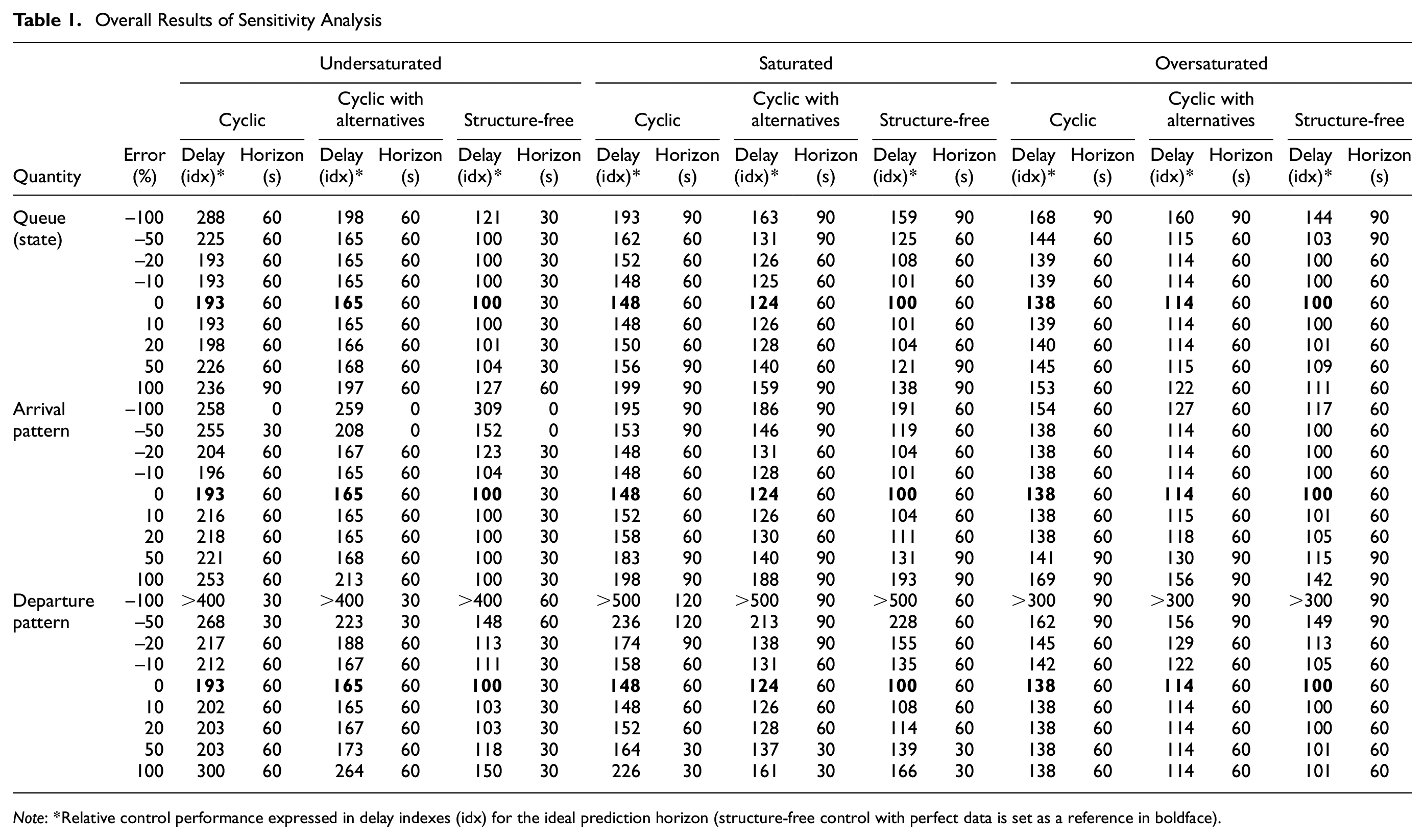
Note: *Relative control performance expressed in delay indexes (idx) for the ideal prediction horizon (structure-free control with perfect data is set as a reference in boldface).

As can be seen in Table 1, in general, increasing errors in the input quantities result in an increase in the total delay of the control system. In the end, an error in the input data results in too short or too long green times, yielding a drop in the performance of the control system. To be able to look in more detail into the behavior of the decrease of performance of the controllers, experimental relations between the delay and the prediction horizon for the different error levels are drawn. The results are presented in Figure 6 for the different control types and different demand scenarios. Only the sensitivity of the cyclic and structure-free controller are presented graphically, the results for the cyclic controller with alternatives can be found in Table 1. As expected, the results of the controller with alternatives lie in general between the results of the cyclic controller (fewer degrees of freedom) and structure-free controller (more degrees of freedom). Note that the experimental relations are presented for the 50% error levels, being extreme, however giving clear insight in the behavior of the system under errors. The behavior is similar for the lower error levels of 10% or 20%, but less extreme, giving less additional delay (see Table 1). The following relations can be observed from the sensitivity analysis (answering the research questions at the beginning of this section):

Figure 6.

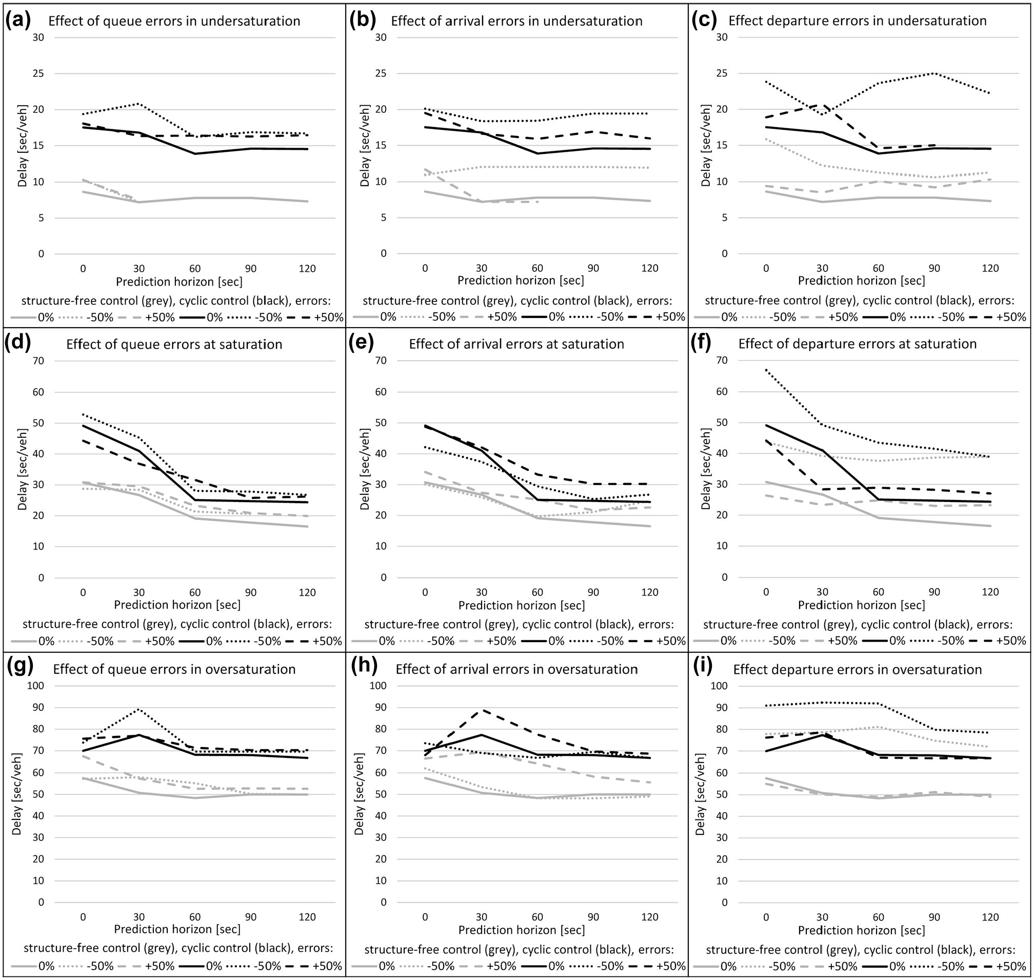
Performance of predictive controllers with errors in the input quantities: queues (left: a, d, g), arrivals (middle: b, e, h), and departures (right: c, f, i), for different demand scenarios: undersaturated (top: a, b, c), saturated (middle: d, e, f), oversaturated (bottom: g, h, i).

Role of the Prediction Horizon

In most of the cases with erroneous input quantities (see Figure 6), prediction still leads to a better performance, that is, the delay is decreasing for increasing prediction horizons. Increasing the prediction horizon can reduce the effect of errors. As can be seen in Figure 6a, in the undersaturated case, the effect of a disturbance in the queue of +50% is eliminated completely for the structure-free controller (and partly for the cyclic controller). This can be explained by the fact that, in the undersaturated case, there are hardly any queues, so an error in the queue information has no large influence (except when completely ignoring the queues as in the −100% case in Table 1).

A reduction of errors for increasing prediction horizons is not guaranteed, however. As can be seen in Figure 6b, in which for the structure-free controller an underestimation in the arrival pattern of −50%, results in a remaining high delay for the larger prediction horizons. In this case, it is better to use no predicted arrivals at all, and purely react to arrived vehicles. Since in the undersaturated case there are hardly any queues, the arrivals are the most important information source. Therefore, errors in the arrival pattern will indeed influence the performance and these errors are accumulated for longer horizons.

Role of the Type of Controller

As can be noticed from Figure 6, in all demand scenarios and for all disturbed quantities, the structure-free controller is not more sensitive to errors in the input data than the cyclic controller. In most cases, the cyclic controller even seems to have a greater drop in performance. There seems to be a trade-off between sensitivity and adaptivity. The structure-free controller, with a high degree of freedom, can adapt better to fluctuations in the traffic conditions than the more constrained cyclic controller. Although a structure-free controller relies more on the erroneous information, because of its adaptivity it can also react and correct mistakes more easily. Therefore, controllers with high adaptivity seem to outperform controllers with low adaptivity, even under erroneous predictions.

Role of the Different Input Quantities

The control system is most sensitive for an error in the saturation flow (departure pattern), especially for an underestimation (–50% error) of the saturation flow, in saturated and oversaturated conditions when queues are present (Figure 6f). Note that in the undersaturated case with hardly any queues an error in the saturation flow can also have a large influence, building up queues quickly (Figure 6c). This sensitivity for the underestimation of the saturation flow can already be noticed at the lower error levels of −10% and −20%, see Table 1.

The system is less sensitive for errors in the current queues and the predicted arrivals. This can be explained by compensating quantities, especially in the saturated case with moderate queues. If there are errors in the queue (Figure 6d), the system can rely on the perfect information on arrivals, and, the other way around, if there are errors in the arrivals (Figure 6e), the system can use the perfect information of the queues. In general, an error in a quantity does not need to be a problem, as long as other information can compensate for this error.

Role of Objective of the Control System

In Figure 6, d–f, especially for the cyclic controller in the saturated case, some counter-intuitive effects can be noticed. For a +50% error in the queues (Figure 6d), or a −50% error in the arrivals (Figure 6e), for short prediction horizons the performance is better than for the reference case of perfect information. This can be explained by the fact that, for short horizons, the total delay costs do not fully represent the real costs encountered when considering the entire horizon. The contribution of queues, especially, is not fully incorporated for short horizons. When there is an overestimation of the queues, or an underestimation of the arrivals, implicitly weights are given to the vehicles in the queue, resulting in more representative costs. This results in an overall decrease in the delay of the control system.

Design Guidelines

From the results of the sensitivity analysis, it becomes clear that prediction indeed improves the performance of a controller if perfect information on predicted quantities is available. The delay of the system decreases for an increasing prediction horizon, and the performance is significantly better than for non-predictive control (considering a very short prediction horizon near zero). Therefore, adding a predictive component is of added value to the control system. However, in real life, the predictive information will never be perfect, and will contain errors. From the behavior of the control system under these errors, as studied in the sensitivity analysis, design guidelines can be defined. The following aspects need to be considered when designing predictive control.

Choice of Prediction Horizon

The choice of the prediction horizon strongly depends on the degrees of freedom of the controller. A more constrained controller asks for a longer prediction horizon to gain the full potential performance out of the controller. The choice of the prediction horizon also depends on the level of saturation. If there are more queues present, control actions have a longer effect in time on the traffic conditions (large time delay of the dynamics in the control system). In this case a longer prediction horizon is needed to consider these effects in the optimization of the performance of the controller.

The choice of the prediction horizon also depends on the quality of the estimated and predicted input quantities of the controller. The use of a longer prediction horizon can reduce the effect of the input errors of the control system, resulting in a better performance. However, there is no guarantee that a longer horizon will automatically reduce the error and not amplify it (see previous section for examples of both effects). Therefore, in the design phase of a controller, using sensitivity analysis can give more insight into the behavior under errors of the controller for increasing prediction horizons, to choose the most convenient length of the prediction horizon.

Choice of Type of Predictive Controller (Degrees of Freedom)

Under perfect information, a predictive controller with a high degree of freedom outperforms the more constrained controllers. There is a trade-off between adaptivity and prediction horizon. A controller with high adaptivity (a high degree of freedom) performs for a short horizon equally well as a controller with low adaptivity and a longer prediction horizon. In the design of the control system, the choice of a more adaptive controller with short prediction horizon or a more constrained controller with a longer prediction horizon can both increase the performance of the system.

Under disturbed conditions, although the controller with a high adaptivity relies more on the erroneous predictions, the controller is also more able to correct its mistakes more easily. There is a trade-off between sensitivity and adaptivity. In the design phase of a predictive controller, sensitivity analysis gives more insight into this interchanging behavior, to be able to choose the most convenient level of adaptivity of the controller.

Note that the choice of the type of predictive controller will also depend on practical implementation issues. A high degree of freedom means a wider decision tree, resulting in longer computation times. A more constrained controller has a smaller decision tree; however, it needs a longer horizon, increasing the depth of the decision tree, which also finally results in longer computation times.

Choice and Quality of Input Quantities

Less accurate predictions do not have to be a problem if another quantity with enough accuracy is available that can be used to compensate the erroneous information. This makes the control system less sensitive for the predicted arrivals and the current queues, as these quantities contain compensating information. The control system is most sensitive for errors in the saturation flow that cannot be compensated by other information.

From the results of the sensitivity analysis, it can also be underlined that it is more important to predict that there is traffic waiting or arriving than how many vehicles are waiting or arriving (especially in undersaturated conditions). As presented in the authors’ earlier work ( 5 ), predicting the arrival times (and probably also the planned turning direction of the vehicles) is more important than an accurate prediction of the number of arrivals. This does not necessarily mean that simplified models that focus more on vehicle presence instead of vehicle numbers (e.g., simplified queue prediction models) achieve a similar control performance, however, to a lesser extent, the errors in vehicle numbers do influence the performance. To what extent a prediction model can be simplified before a substantial decrease in the performance occurs needs to be investigated in more detail.

Choice of Objective of the Control System

The results in this paper are obtained for a predictive controller optimizing the delay of the traffic system. The choice of the control objective may influence the control decision and therefore the performance of the control system. However, most control strategies and objectives depend on the same quantities of the traffic system, like delay, number of stops, number of vehicles in the queue, and so on. Also, the traffic dynamics (queue formation) plays an important role in practically all formulations of performance of the control system, which is independent of the specific objective function. Therefore, mostly similar behavior for these control systems is expected in the sensitivity of the considered input quantities in this paper (predicted arrivals, predicted departures, measured queues).

In any case, it is important that the objective of the control system should represent the true costs of the control system for the entire horizon. If not, this can lead to counter-intuitive effects for shorter prediction horizons when input quantities are disturbed. Therefore, it may be helpful to include end costs in the objective function, reflecting the additional costs that vehicles will encounter beyond the limited prediction horizon (e.g., include end costs for queues that are still present at the end of the prediction horizon). It is left for further research to determine if this really limits the influence of information errors and leads to more robust controllers.

Conclusions and Recommendations

In this paper, an experimental framework was proposed to investigate the sensitivity of signalized traffic controllers for erroneous input quantities. The framework was illustrated for predictive control on a single intersection under different demand scenarios. Experimental relations between the performance of the control system and the prediction horizon were obtained for perfect information and erroneous input data. Different input quantities were structurally disturbed, concerning queue lengths (current state), number of predicted arrivals, and departures (saturation flow). These relations were studied for different types of predictive controllers with increasing levels of adaptivity (degrees of freedom), varying from cyclic to structure-free control.

The results show that prediction improves the performance of a signalized traffic controller, even in most of the cases with erroneous prediction information. Increasing the prediction horizon reduces the effect of errors and compensates errors with the information available from undisturbed predicted quantities (e.g., arrivals compensate queue information and vice versa). Therefore, controllers seem to be more sensitive to errors in stand-alone quantities (saturation flow in particular) that cannot be compensated by other information. Furthermore, controllers with a high adaptivity, and therefore a high ability to anticipate fluctuating traffic patterns, are not necessarily more sensitive to prediction errors. Although these controllers rely more on the erroneous information, controllers with high adaptivity can also react and correct mistakes more easily. Therefore, controllers with high adaptivity seem to outperform controllers with low adaptivity, even under erroneous predictions.

The outcome of the sensitivity analysis contributes to understanding the relations between information quality and performance of signalized traffic control. In the design phase of a controller, this insight can be used to make choices on the length of the prediction horizon, the level of adaptivity of the controller, the representativeness of the objective of the control system, and the input quantities that need to be estimated and predicted the most accurately.

The final goal of future research will be, on the one hand, to decide how accurate estimation and prediction methods should be to be of added value for signalized traffic control, and on the other hand, to be able to develop signalized traffic controllers that are robust to input errors. To this end, more experiments in this framework need to be done to analyze the effect of errors in the estimated and predicted input quantities on the performance of the controller. The experiments will be extended by disturbing quantities in different and more realistic ways as will be encountered in real life, like shifts in arrival times and directions, by introducing a random noise, and by combining errors of different quantities simultaneously. The experiments will be extended from a single intersection to coordinated intersections and finally a network context to represent real-life cases.