
Abstract
Urban deliveries are traditionally carried out with vans or trucks. These vehicles tend to face parking difficulties in dense urban areas, leading to traffic congestion. Smaller and nimbler vehicles by design, such as cargo-cycles, struggle to compete in distance range and carrying capacity. However, a system of cargo-cycles complemented with strategically located cargo-storing hubs can overcome some limitations of the cargo-cycles. Past research provides a limited perspective on how demand characteristics and parking conditions in urban areas are related to potential benefits of this system. To fill this gap, we propose a model to simulate the performance of different operational scenarios—a truck-only scenario and a cargo-cycle with mobile hubs scenario—under different delivery demand and parking conditions. We apply the model to a case study using data synthesized from observed freight-carrier demand in Singapore. The exploration of alternative demand scenarios informs how demand characteristics influence the viability of the solution. Furthermore, a sensitivity analysis clarifies the contributing factors to the demonstrated results. The combination of cargo-cycles and hubs can achieve progressive reductions in kilometers-traveled and hours-traveled up to around densities of 150 deliveries/km2, beyond which savings taper off. Whereas the reduction in kilometers-traveled is influenced by the the carrying capacity of the cargo-cycle, the reduction in hours-traveled is related to to the cargo-cycle ability to effectively decrease the parking dwell time by reducing, for instance, the time spent searching for parking and the time spent walking to a delivery destination.
Urban deliveries are traditionally carried out using motor vehicles such trucks, a term that we will use to encompass the use of vehicles such as vans, lorries, or others that are similar. Such conventional urban delivery method is increasingly under pressure. Because of the increase in urban population and the rise of e-commerce, delivery demand has not only increased, but also shifted toward smaller consignments shipped at a higher frequency ( 1 ). However, urban transport infrastructure supporting city logistics distribution has often remained unchanged. In particular, trucks often lack available curb-space for parking and loading/unloading in urban areas, with the consequence of increasing cruising for parking, dwell times (as a result of increase in walking distance), and unauthorized parking ( 2 ). With the increase in urban population density, traffic congestion levels have also increased, negatively affecting truck travel times ( 3 ). To reduce the negative externalities caused by trucks in urban areas, including road blockages caused by unauthorized parking and noise and air pollution, city authorities have often taken regulatory actions imposing parking and travel restrictions for trucks in urban areas ( 4 ). These factors lead to an increase in delivery costs, negative social and environmental impacts, or both.
An alternative to the use of conventional trucks to perform urban last-mile deliveries that has been deployed in several cities around the world (5–7) relies on the complementary use of cargo-cycles, sometimes supported by mobile hubs. We use the term cargo-cycles as encompassing of two, three and four wheelers, which have some component of human-based propulsion, often with electric motor support. Mobile hubs are small de-consolidation centers which, differently from traditional urban consolidation centers, often do not require a fixed infrastructure, except pre-existing parking space. In this case, trucks carry consolidated delivery loads from a depot to central areas, more specifically to the hubs, from which cargo-cycles pickup the goods and delivery locally to the final destinations.
The use of cargo-cycles is commonly assumed to be comparatively more agile than trucks, as these vehicles require a smaller parking space, can access areas and routes not accessible to trucks, and can park closer to destination. This is particularly advantageous in settings of heavy parking and traffic congestion, as these vehicles can lead to reduced cruising for parking and unauthorized parking if due care is taken in their use and adequate regulations are in place. On the other hand, the cargo-cycle is disadvantaged with respect to trucks as it able to carry less cargo and it reaches a lower maximum travel speed, being more suited to deal with smaller consignments and higher delivery densities (deliveries per km2). In fact, past research showed mixed results on whether a cargo-cycle-based distribution system can bring about improvements compared with the traditional truck-based system. According to a literature review, 47% of the studies reviewed proposed the use of bicycles/tricycles as alternative vehicles to perform last-mile deliveries instead of the conventional alternative ( 8 ).
In this study we seek to answer the following research question: how do delivery demand and parking conditions relate to the benefits of using a cargo-cycle-based distribution system when compared with the conventional truck-based system? In this setting, we investigate how demand characteristics, particularly delivery density, parcel weight, and parking conditions, particularly the excess dwell time resulting from cruising for parking and walking, influence the performance of a system of cargo-cycles with mobile hubs, when compared with truck-based deliveries, in “last-mile” operations. For this purpose, we develop a simulation method that allows replicating to a suitable extent the delivery tours of a freight carrier in urban areas for both a truck-based system and a cargo-cycle-based system with mobile hubs, under different delivery demand and parking conditions. The simulation method is based on detailed data for delivery trips performed by trucks of a parcel delivery company in downtown Singapore. The simulation method first takes trip records as an input to generate a delivery demand with given characteristics (location, quantity, time window). Then, given a delivery demand, it simulates two operational scenarios: (a) a truck-only distribution scenario and (b) a cargo-cycle with mobile hubs distribution scenario. The truck-based distribution estimates are compared with the real data for validation. The data are also used to infer the traveling, cruising, and parking durations. For the latter two we assume a reduction when using cargo-cycles. For varying demand characteristics, we compare the two scenarios using several performance metrics (total daily travel distance and time; total daily operating time, which includes travel time and dwell time; and the number of vehicles required). We also perform a sensitivity analysis on three key model parameters as to better understand their contribution to predicted total travel distance and operations time.
In the following section we review the relevant literature. Then, we describe the truck trips data and the simulation model developed. Further, we present the results of the model validation, of the simulated scenarios, and of the sensitivity analysis. We conclude with a discussion of the results.
Literature Review
Whereas some research focuses on the potential and factors that can lead to or restrict the adoption of cargo-cycles ( 9 , 10 ) our focus is on the operational impact of adopting this alternative mode. In this domain, a large part of the research focuses on environmental impacts compared with conventional delivery operations. Sadhu et al. analyzed the data collected from 2,000 cycle rickshaw trolley (CRT) drivers in Delhi in 2011 and showed that CRTs for city goods movements reduced fuel use and vehicle emissions ( 11 ). Saenz et al. compared the carbon footprint of a cargo-cycles logistics service with that of a traditional system ( 12 ). The results showed that total greenhouse gas emissions reduced between 51% and 72% in the cargo-cycles system. Figliozzi and Tipagornwong presented a lifecycle emissions minimization model, concluding that using small cargo-cycles in dense service areas, for relatively small loads, and when the depot is located close to the delivery area, can obtain the lowest lifecycle emissions ( 13 ).
There is also considerable attention to financial impacts and operational impacts. Melo and Baptista developed a microsimulation model to replicate traffic conditions and estimate cargo-cycles environmental and operational impacts ( 14 ). The results showed that the use of cargo-cycles improves mobility, environment, energy consumption, and running costs if deployed at the appropriate spatial scale within the city. Marujo et al. examined the cost and environmental impacts of mobile-depot-based delivery using GPS data ( 15 ). They showed that the use of cargo-cycles and mobile depots in the last-mile delivery led to significant reduction of greenhouse gas emissions and local air pollution. In addition, the mobile-depot-based delivery setup yielded a slight cost reduction over the traditional setups. Nascimento et al. assessed the economic viability of cargo-cycles from the carrier’s perspective, concluding possible benefits despite several contextual barriers to adoption in Brazil ( 16 ). Arnold et al. simulated a cargo-cycle system for B2C e-commerce distribution in a comparative setting with pickups from lockers, and with a hybrid system of cargo-cycles and lockers against conventional deliveries ( 17 ). The authors focused on a comparison of internal and external costs across the delivery strategies. The study revealed that diminishing external costs requires an increase of internal costs by the carriers. Gruber and Narayanan compared the travel time difference between cargo-cycles and conventional vehicles in commercial transport, applying a regression model ( 9 ). The results indicate that when the trips distance is short, the cargo-cycles and cars performances overlap. The increase of the trip distance made cars more advantageous. However, the time to park, which might be comparatively larger for trucks and contributes to the vehicle dwell time, was a neglected element in their research. Tipagornwong and Figliozzi analyze the competitiveness of cargo-cycles against diesel vans in urban areas using a cost model and considering two demand scenarios ( 18 ). The results indicate that (a) cargo-cycle competitiveness is affected by drivers’ costs assumptions, and (b) specific local conditions such as parking difficulties, low travel speeds, and time-constrained delivery windows can contribute to widen the gap between the delivery modes. Similar conclusions about the scenarios in which cargo-cycles are more promising are achieved by Conway et al. ( 5 ) and Choubassi et al. ( 19 ). The latter highlighted factors such as high delivery density and congested areas as well as the presence of depots within the delivery areas as contributing factors to the comparatively better performance of the cargo-cycles. To the best of our knowledge no study could be found that explores in detail the relationship between the performance which the system of cargo-cycles can achieve and demand characteristics relating to delivery density and parcel/delivery weight distribution.
Methods
Data Description
For estimating delivery demand, we used the records of about 20,000 deliveries performed over 3 months by a parcel delivery company in the central business district (CBD) of Singapore, a 2.3 km2 urban area. For each delivery, the delivery weight (in kg), delivery destination GPS location, and delivery priority level are available (“high” priority consignments have to be delivered by noon, “low” priority consignments can be delivered anytime). Moreover, each record reports the date when the delivery took place, two timestamps at the start/end of the delivery time, and a unique ID of the vehicle used to perform the delivery.
Note that when a truck is parked, the driver might perform more than one delivery, walking between different delivery locations, before returning to the truck. We therefore rely on the concept of “delivery groups,” explained as follows. Delivery locations are first mapped to buildings. Then, deliveries that took place consecutively in time, within the same building, and performed from the same vehicle are aggregated into a single “delivery group,” which indicatively corresponds to a group of deliveries performed in a single parking event, that is, without moving the vehicle from the chosen parking location. This process leads to a set of 8,300 delivery groups from the original dataset of about 20,000 deliveries. The total shipment weight delivered in a delivery group is the sum of the individual weights of the deliveries associated with that group. For simplicity, we address delivery groups as “deliveries” throughout this paper.
Travel distances between consecutive deliveries are obtained by computing the shortest path between each pair of locations, and the respective travel times are obtained by querying the Here Maps API (here.com) for the historical travel time between each pair of locations.
We estimated the vehicle dwell times from the individual deliveries start/end timestamps as show in Figure 1. Consider two deliveries, named
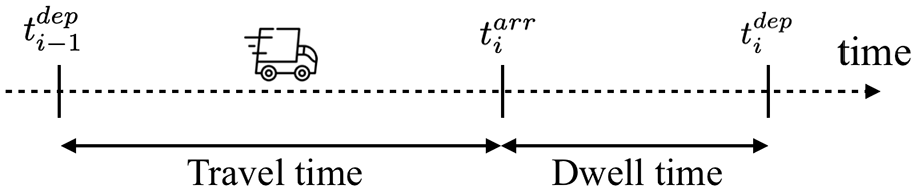
Method used to estimate vehicle dwell times.
The resulting dwell time distribution is right skewed with a mean and median dwell time of 7.6 and 16 min, respectively (see histogram in Figure 2). It is important to note that the resulting dwell time estimates include not only the times to deliver the consignments but also other activities including cruising for parking (i.e., time spent searching for available parking), queuing, and walking time to the consignee. Later in the paper we will assume that, by using a cargo-cycle, the vehicle dwell times are reduced—because a cargo-cycle can park closer to a destination, therefore reducing walking time, and does not cruise for parking—with respect to trucks.
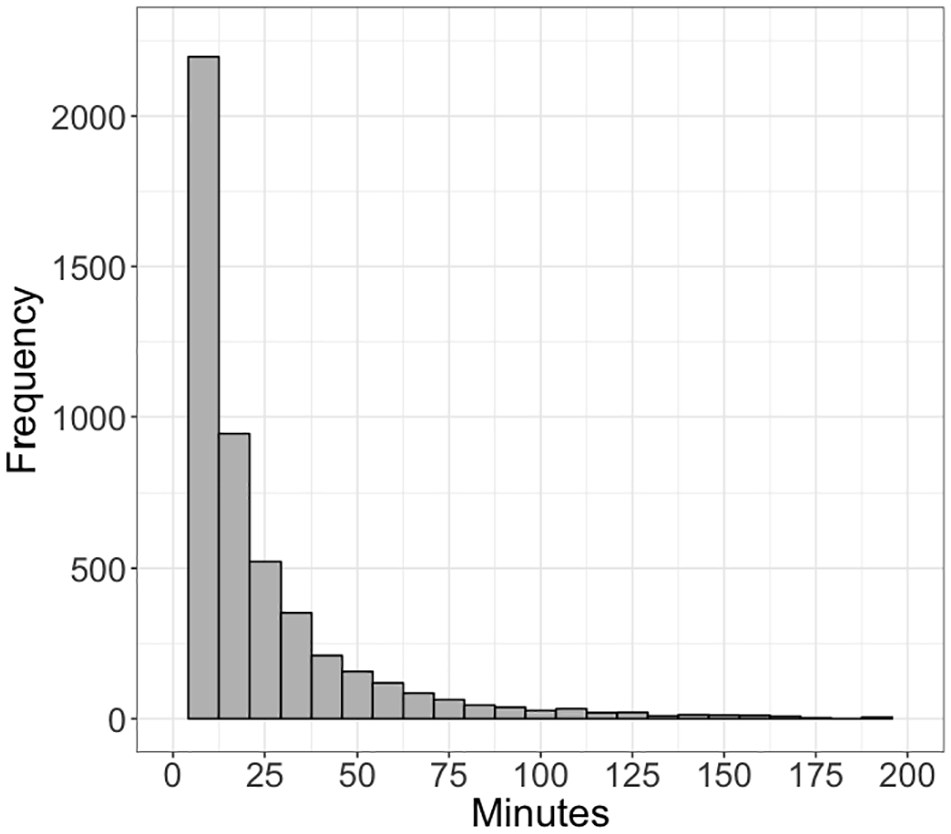
Empirical distribution of the estimated dwell times.
Overview of Simulation Model
The simulation model developed consists of three sub-models (Figure 3):
a demand generation model that generates delivery demand scenarios based on (i) a real-world dataset of daily deliveries performed by a freight carrier and (ii) a set of parameters (demand density and delivery weight distribution) characterizing the desired demand scenario;
a (tour) scheduling model that organizes the generated delivery locations into time- and distance-efficient freight vehicle tours;
a vehicle assignment model that calculates the minimum number of vehicles (either trucks or cargo-cycles) required to perform all scheduled tours.
Both demand-specific inputs characterizing the demand scenarios and the desired operational scenario (i.e., the way deliveries are performed) need to be specified to operationalize the model. It should be noted that the proposed method to generate tours does not aim to compute optimal delivery tours, for example, tours with the minimum travel distance and time. Our intention is to replicate, to some extent, the actual tours observed to be performed by the freight carrier. Details on this comparison are provided in the Operational Scenarios section.
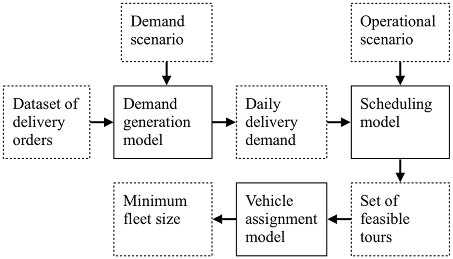
Simulation flow (dashed: inputs/outputs, solid border: models).
Simulation Sub-Models
Sub-model 1: Demand Generation
Delivery demand for a hypothetical weekday is generated based on the records of 8,300 delivery groups. A demand scenario is characterized by (i) a demand density (number of deliveries per km2 for the study area), and (ii) a delivery weight distribution. To generate demand with a given number of deliveries, we re-sample without replacement the original dataset of delivery records. To simulate different delivery weight distributions, we multiply the original weights of the sampled deliveries by a positive constant. We assume the dwell time remains as per prior estimates.
Sub-model 2: Tour Scheduling
In the tour scheduling sub-model, deliveries are organized into tours. The procedure to construct distance- and time-efficient feasible tours consists of three steps: (1) Clustering (2), Feasible tour search and (3) Tour merging. The procedure takes two main inputs: first, the daily delivery demand generated in the previous demand generation sub-model, and second, the characteristics of the operational scenario simulated, including the type of vehicle used (truck or cargo-cycle) and the related vehicle constraints (e.g., vehicle weight capacity, maximum speed). The Operational Scenarios section provides a detailed description of the different operational scenarios simulated.
In the Clustering step the objective is to group a given set of deliveries into disjoint clusters, each representing a potential tour. We use a hierarchical clustering algorithm to generate a hierarchy of nested clustering solutions. At the lowest level of the hierarchy, there are as many clusters as the number of deliveries; at the highest level, all deliveries are grouped into a single cluster; any intermediate level is generated by merging two clusters generated at the lower level. We aim to generate clusters which are not only geographically compact, but also which contain deliveries of the same priority level. For this, the algorithm requires as input a distance matrix
Once clusters are defined, in the next step of Feasible tour search, a tour is feasible when it satisfies the following constraints: (i) the total weight of all deliveries in the tour is less than or equal to the vehicle weight capacity, (ii) the total time it takes for a vehicle to perform the tour is less than or equal to the maximum vehicle operating time (assumed shift time), (iii) the total tour-distance traveled is less than or equal to the maximum vehicle travel distance (important for cargo-cycle range), and (iv) all high-priority deliveries are scheduled before noon. The upper bounds in constraints (i)–(iii) are vehicle-specific, and therefore depend on the mode of transport (i.e., trucks or cargo-cycles). The tour travel distance and time are computed by finding the shortest path covering all delivery points of the tour, starting and ending at the depot (for trucks) or at a consolidation hub location (for cargo-cycles), and assuming an average travel speed. The shortest path is found by solving a traveling salesman problem for each cluster. To satisfy constraint (iv), if a tour contains at least one delivery with high priority, we limit the maximum tour time to the length of the morning shift, such that the whole tour can be completed before noon. We iteratively search for the largest clusters satisfying all the above constraints from the hierarchy of clustering solutions. We therefore start from the top of the hierarchy and iteratively check, for each cluster in the clustering solution associated with the given level of the hierarchy, whether its associated tour is feasible. Feasibility leads to the cluster’s deliveries being assigned to a tour; otherwise, we proceed to a lower level of the hierarchy, that is, splitting the cluster into smaller nested clusters. The search stops when all deliveries are assigned to feasible tours. In the operational strategy that involves the use of the cargo-cycles, deliveries need to be assigned to the respective hub location. To do so, we start the search for feasible tour not from the top of the hierarchy of clustering solution, but from a lower level, specifically from the level containing as many clusters as the desired number of hubs, and then search for feasible tours within each cluster.
Lastly, for Tour merging the objective is to overcome tours that are undesirably small (containing few deliveries), therefore forcing the vehicle to return to the depot (or the consolidation hub in case of cargo-cycles) more often than needed. To form larger tours, we consider all possible pairwise combinations of the identified feasible tours and identify those in which merged tours are (i) feasible tours and (ii) their total tour travel distance and time are smaller than those of the original tours combined. We then model the possible tour combinations as a bipartite graph in which nodes represent the tours and links connecting pairs of tours represent the feasible combinations. Then, the maximum matching of the graph is obtained to find the largest possible number of combinations. We then merge the selected matches into single tours. We repeat the pairwise merging of tours until there are no additional feasible combinations.
Sub-model 3: Vehicle Assignment
After we generate efficient and feasible tours, we find the minimum number of vehicles needed to perform all tours. We start from an initial number of vehicles equals to the number of tours. We then solve two bin-packing problems sequentially, in which tours are assigned (“packed”) to a minimum number of vehicles (“bins”), in which the “capacity” of each vehicle consists of the length of a driver’s working shift. We assume a driver shift starts at 7 a.m. and ends at 5 p.m. In the first bin-packing problem we assign high-priority tours (i.e., tours that contain at least one high-priority delivery, meaning the whole tour needs to be completed by noon) to vehicles, assuming that each vehicle has an initial “capacity” to perform the high-priority tours within 5 h (assuming vehicles start at 7 a.m.), therefore guaranteeing that high-priority tours are dealt with within the morning shift. In the second phase we add to all vehicles 5 h of “extra capacity” (assuming the afternoon shift starts at 12 p.m. and ends at 5 p.m.) and assign the remaining low-priority tours to vehicles solving a second bin-packing problem. Finally, we retain only those vehicles to which at least one tour was assigned. As a result, we obtain the minimum fleet size needed to perform all tours, such that all high-priority tours can be completed in the morning.
Operational Scenarios
We simulate the two operational scenarios: a truck-only scenario (which is validated against the baseline scenario) and a truck+cargo-cycle scenario. The first scenario simulates a traditional distribution system relying solely on trucks (scenario truck-only). Truck tours start and end at a depot, located about 20 km from the area where deliveries are performed. These tours are validated against real data by computing the total travel distance and operating time and comparing them against the same metrics derived from the carriers’ data. We refer to the real tours performed by the delivery company as the baseline (scenario baseline) which we expect our algorithm to replicate to a reasonable extent (scenario truck-only).
The alternative scenario simulates the use of a hybrid system of trucks and cargo-cycles (scenario truck+cargo-cycle): trucks are used to carry consolidated loads from the depot to a mobile hub (hereafter called “hub”) located in the CBD; cargo-cycles pick up the consolidated loads at the hubs and perform the individual deliveries. Note that in this scenario, trucks are used only to deliver consolidated loads to the hubs and are not used for delivering to the final destinations, and only cargo-cycles are used to perform the last leg of the chain. Therefore, we do not consider the case of a mixed cargo-cycle and truck scenario in which both vehicle types are used for the last mile. Hubs are assumed to be similar to containers in form and fit within a car parking space. For the presented results, we assume the deployment of two hubs. Each hub contains a maximum of nine cargo-cycle loads. The geographical locations of the hubs change depending on the daily demand scenario and are determined by the simulation model. Each hub is placed at the geographical center of the demand cluster of deliveries served by the hub. Given that cargo-cycles are more compact and nimbler and therefore able to find a parking space easily, their dwell times are assumed to be 40% less compared with those of trucks. This is a conservative assumption, as past research reports dwell time savings of 75% ( 20 ). It should be noted that, as mentioned earlier, our dwell time estimation includes the time for cruising and queuing for parking. The original maximum weight a cargo-cycle can carry is 205 kg. However, recognizing that the heterogeneous volumes and shapes of the delivery packages might not allow the cargo-cycle to be loaded to maximum capacity, we assume that only 70% of the maximum carried weight can be loaded. Table 1 summarizes the input parameters for each mode.
Assumptions of Mode-Specific Parameters
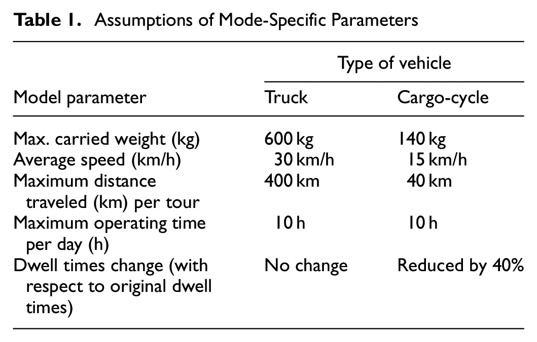
The two alternative operational scenarios are tested on different demand scenarios, characterized by a given demand density and delivery weight distribution. In the baseline case, daily demand densities range between 25 and 90 deliveries per km2, the mean delivery weight is 5 kg and median weight is 1.1 kg. Each demand scenario is simulated 50 times, and the resulting outputs are averaged across simulation runs.
Performance Metrics and Sensitivity Analysis
The model outputs a set of metrics describing the operational performance of the simulated freight distribution. These are: (a) total daily travel distance and time; (b) total daily operating time, which includes travel time and dwell time; and (c) the number of vehicles required.
Further, we analyze the sensitivity of some output metrics—total travel time and operating time—to input parameters. We test two vehicle-specific inputs: dwell time reduction and capacity for the cargo-cycles and a demand-specific input, the prior mentioned constant that multiplies the original delivery weights. We take a one-factor-at-a-time approach, changing one of the four parameters each time, from −50% to 50% with a 10% increment to the baseline value reported in Table 1, keeping the other parameters fixed.
Results
Validating the Baseline Case
Figure 4 shows the output metrics for validation scenarios (baseline and truck-only), using as input the observed delivery demand. The baseline scenario illustrates the distance and time that the freight carrier took to perform the deliveries, following the observed vehicle assignment and delivery sequences in the data. The truck-only scenario is obtained by simulation, using the same real demand as input. Note in this case the demand generation model is not run and results are averaged by day of the week. The daily travel distance of the simulated truck-only scenario is on average 28% less, and the total operating time is 12% less than in the baseline scenario. This difference can potentially be explained by some factors which cannot be accounted for in the simulation, such as:
Deviation in real-world delivery tours performed by the drivers from optimal tours. These might have been because of receiver-related factors (e.g., the receiver was not available at the moment of the delivery) or driver-related factors (e.g., driver might prefer to deliver bulky items first even if they are not high priority as that would free space in the van and ease subsequent load/unloads)
Exceptional traffic congestion conditions, parking congestion conditions
Operational practices such as having smaller vans re-loading from larger vans during daily operations
Naïve assumption of shortest path routes
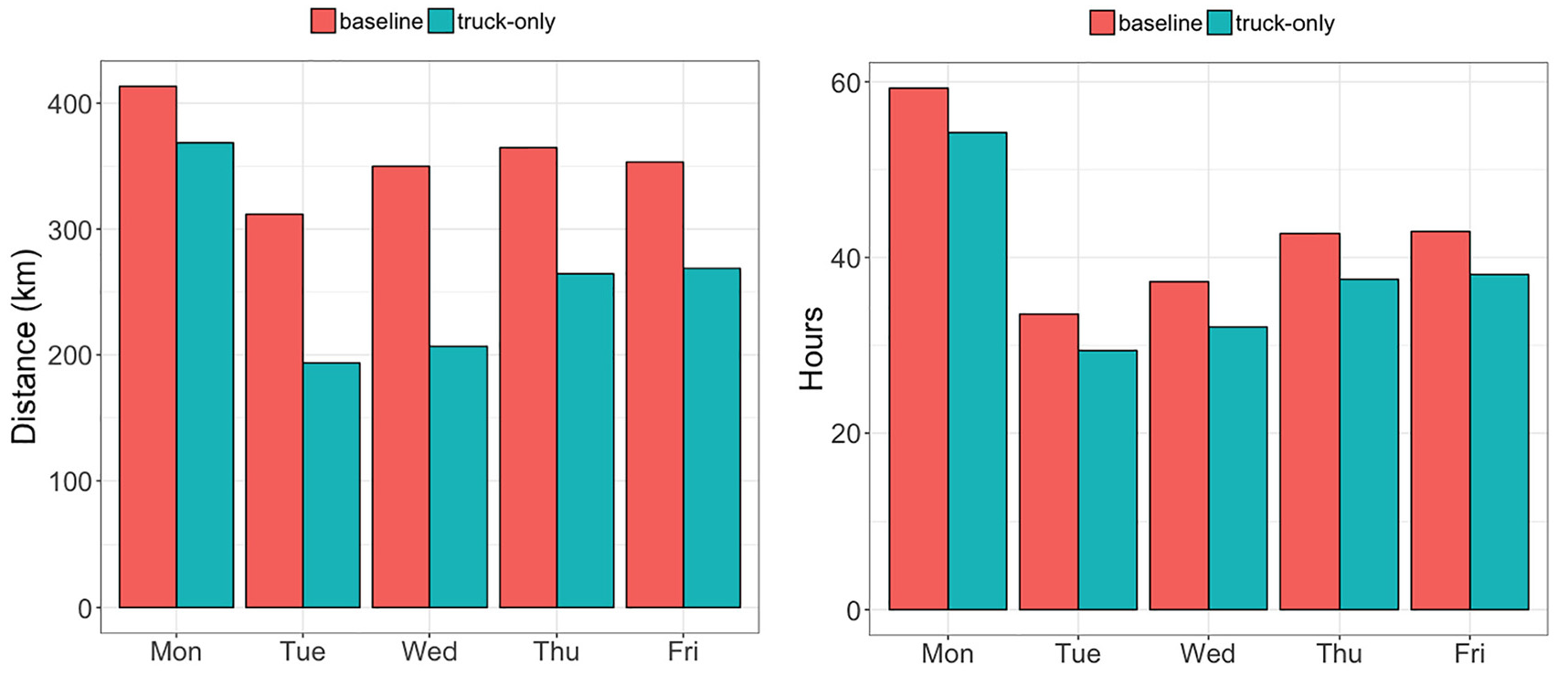
Daily total distance traveled (left) and the daily total operating time (right) for the baseline (observed data) versus truck-only scenario (simulated).
Despite this, we conclude that the simulation model can replicate to a reasonable extent the performance of carrier tour planning. Note that this comparison is performed for averaged metrics across days of the week, whereas for the following analysis we draw random delivery groups from any given day of the workweek.
Simulation-Based Analysis
Figure 5 shows the mean percentage change in travel distance and operating time obtained by using cargo-cycles (truck+cargo-cycle scenario), versus the truck-only scenario, for varying demand density conditions and different delivery weight multipliers. We observe a steep decrease of both travel distance and operating time as the demand density increases from 25 delivery/km2 to about 150 delivery/km2, reaching a 75% decrease in travel distance and a 40% reduction in total operating time (given the original weight distribution). After this point, the savings in total operating time and travel distance stabilize as demand density increases.
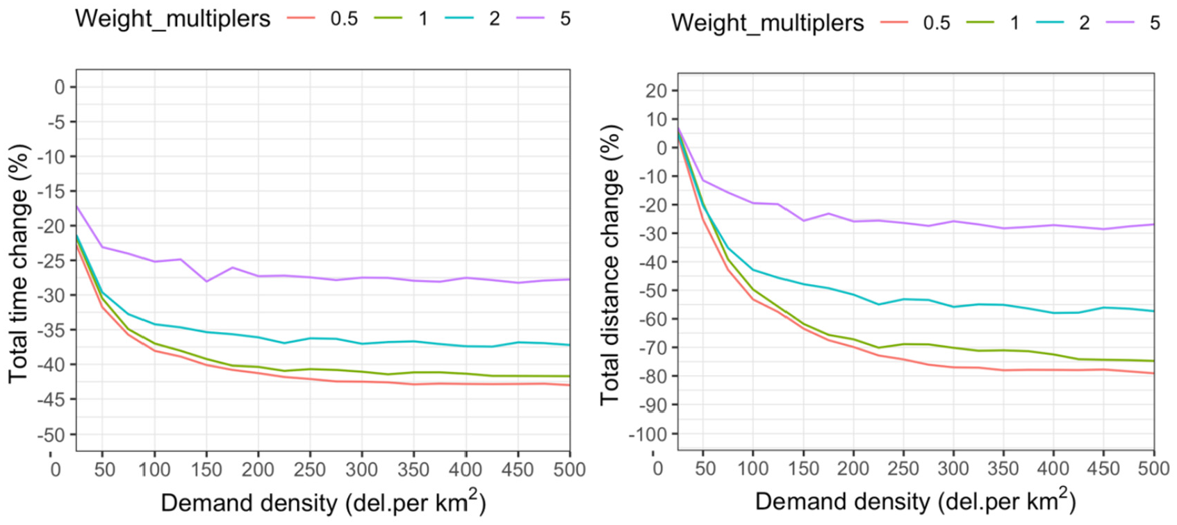
Travel distance (left) and time (right) savings for cargo-cycle solution with respect to a truck-based solution.
We also observe that heavier weights influence the performance, especially if combined with larger demand densities. As the delivery weight distribution shifts toward heavier weights, the improvements brought about by the cargo-cycle system become less significant.
Figure 6 compares the average minimum fleet size required to fulfill daily demand, for the two distribution scenarios and for varying demand density. The smaller fleet of cargo-cycles can be explained as a product of the method, which minimizes the distance traveled and operating time but not the fleet size itself. Firstly, cargo-cycles tours are shorter as these pick up the goods from hubs located in the CBD, and do not require traveling back to the depot. Since our method attempts to add multiple tours to each vehicle, shorter tours can lead to a more efficient use of vehicles. On the other hand, the method is detrimental to the metrics of truck fleet required, because longer tours leave less opportunities for matching in light of existing schedules and maximum operating time per day parameter.
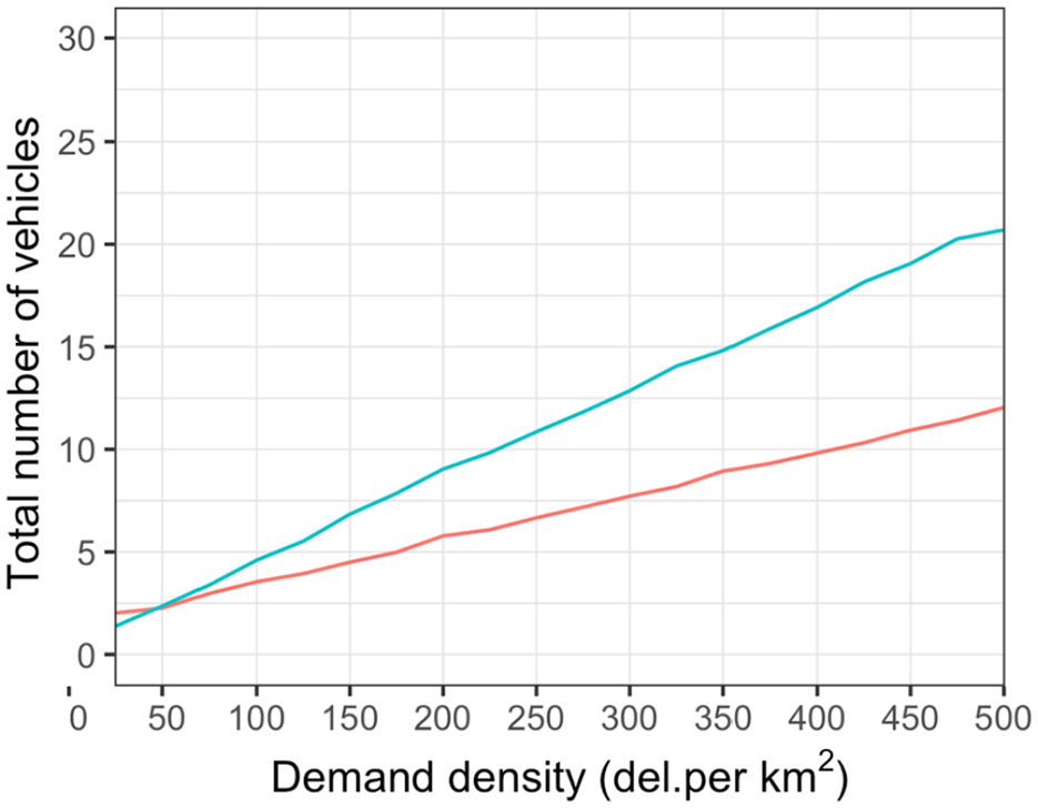
Mean fleet size for truck-only (blue) and truck+cargo-cycle (red) scenario.
Sensitivity Analysis
We perform a sensitivity analysis for three key parameters to better understand their contribution to predicted total travel distance and operations time, with results illustrated in Figure 7. The selected parameters are (1) the capacity of cargo-cycles, (2) cargo-cycle dwell time, and (3) weight multiplier factor of parcels. In these tests, we fix the demand density at 100 deliveries per km2. Note that concerning total travel distance, this result is highly dependent on the assumption of the depot location; for example, in the truck+cargo-cycle scenario, trips to/from the depot contributed on average 70% of the total distance traveled.
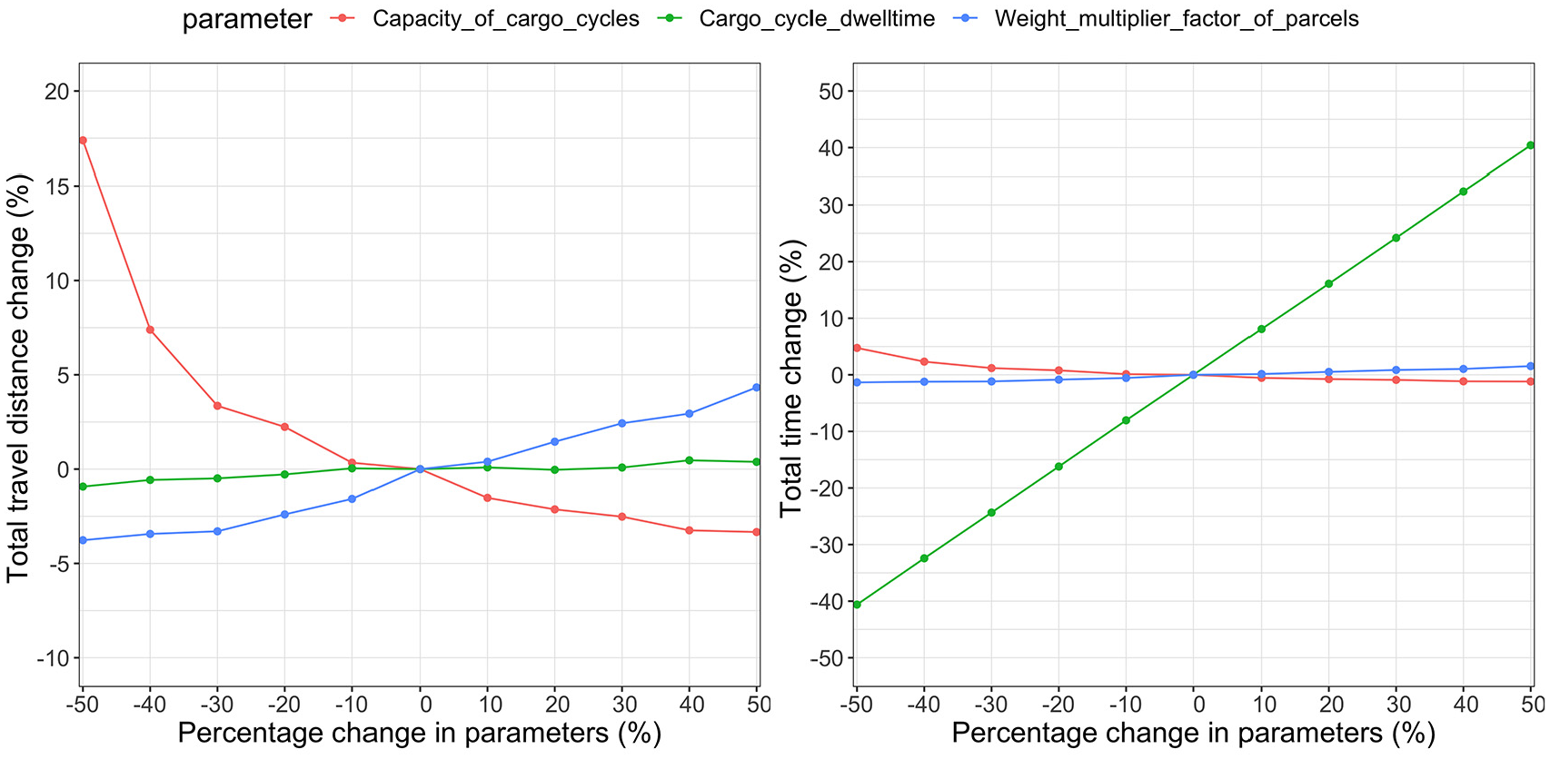
Sensitivity analysis results.
The results for the selected parameters’ influence on total travel distance demonstrate a major effect by the assumed carrying capacity and minor effects from the assumed dwell times and delivery weight. Looking at reductions in capacity, a 50% reduction (to 70 kg) can lead to 17% increase in travel distance. On the other hand, increases in capacity have a small impact. With regards to total operational time, the only critical factor is the assumption of dwell time savings associated with cargo-cycle use. This is justified mainly as the dwell time contributes, on average, to more than 75% of total operational time. In addition, the reduction in dwell times can also increase the number of deliveries that can be completed in a single tour, which to some extent influences the fleet size required to fulfill the demand.
Conclusion
We developed and applied a quantitative method to assess how delivery demand conditions relate to the benefits of using a cargo-cycle-based distribution system when compared with the conventional truck-based system. We estimated the benefits in relation to total distance traveled, total operating time, and fleet size. Decreases in all metrics can be justified as proxies for a more sustainable freight distribution strategy. This method is applied in a simulation context informed by a dataset of real deliveries performed in the highly urbanized setting of Singapore’s CBD.
In line with recent experiments we found that the introduction of cargo-cycles for last-mile distribution, supported using mobile hubs, can lead to considerable benefits. However, this is clearer under specific demand scenarios, particularly at higher demand densities and lower shipment weights. As delivery density increases from low density to up to around 150 deliveries per km2 the cargo-cycle based system shows increasing improvements (reduction in total operating time and distance traveled). Beyond this delivery density we observe a stabilization of the cargo-cycle-derived performance improvements compared with a truck-only system. However, these results depend on several factors. Note that actual delivery density would be equal or higher than the used values, as we grouped deliveries performed by the same vehicle in the same stop as the unit of analysis. Furthermore, the starting baseline distribution of observed delivery weights shows that most of the deliveries recorded are light (median weight is 1.1 kg). Most of the deliveries remain relatively light even when we simulated heavier weights (by multiplying the original delivery weights by a constant), but these hinder the benefits of a system using cargo-cycles and mobile hubs. The distribution of heavier weights was shown to sometimes hinder any improvement, which supports the hypothesis that this distribution system is more suited for parcel deliveries, which is timely considering e-commerce growth. Finally, we assumed that the cargo-cycles are associated with a reduction in delivery times of 40% with respect to trucks. Albeit conservative, this reduction should be expected if the cargo-cycles are able to park closer to the delivery destinations and are not affected by parking congestion. To conclude, if demand density is low, the benefits are expected to be fewer, and if a city is not affected by heavy parking congestion, or the cargo-cycles are affected as much as truck by parking congestion, the benefits obtained by the use of cargo-cycles are expected to be more limited.
Taking the baseline case for the freight carrier (with a demand density between 25 and 90 deliveries per km2), the total fleet size needed can be reduced by up to 36%. Moreover, the total distance traveled can be reduced up to 70%, and the total operating time up to 40%.
Considerations for operating costs and other influencing factors were not explored in this research. For instance, an important factor to take into consideration when switching to a cargo-cycle with mobile hubs system is the need for extra space closer to the delivery locations. Although these need not take the form of a fixed infrastructure, the cargo-cycles still need to be parked overnight and require charging stations. Moreover, throughout the day the mobile hubs need to occupy the space equivalent to a single parking slot. We cannot ignore that larger scale deployment of cargo-cycles might shift the traffic and parking management concerns to curb-space management. We put forward as future research the exploration of the impacts of wide-scale adoption of cargo-cycles from a traffic flow and curb-space management perspective, as well as giving consideration to the impacts of street network design on the presented results.
Footnotes
Acknowledgements
This work is supported in part by the SUTD-MIT International Design Centre (IDC). We thank our partners, RYTLE GmbH and United Parcel Service Singapore Pte Ltd (UPS), for sharing data and insights. We also thank Ming Hong Chua and Zhiyuan Chua for the support provided in data analysis and processing. Any findings, conclusions, recommendations, or opinions expressed are those of the authors only.
Author Contributions
The authors confirm contribution to the paper as follows: study conception and design: Dalla Chiara, Alho, Cheah and Ben-Akiva; simulation model development: Dalla Chiara and Cheng; analysis and interpretation of results: Dalla Chiara, Alho, Cheng and Cheah; draft manuscript preparation: Dalla Chiara, Alho, Cheng and Cheah. All authors reviewed the results and approved the final version of the manuscript.
Declaration of Conflicting Interests
The author(s) declared no potential conflicts of interest with respect to the research, authorship, and/or publication of this article.
Funding
The author(s) disclosed receipt of the following financial support for the research, authorship, and/or publication of this article: This work is supported in part by the SUTD-MIT International Design Centre (IDC), under the grant IDG21800101, under a project titled “Data-Driven Design of Last-Mile Urban Logistics Solutions to Address E-Commerce Growth”.
Data Availability
The data that support the findings presented here were used under license for the current study. As such, the data are not publicly available.