Empirical Study on the Properties of Adaptive Cruise Control Systems and Their Impact on Traffic Flow and String Stability

Abstract

Adaptive cruise control (ACC) systems are standard equipment in many commercially available vehicles. They are considered the first step of automation, and their market penetration rate is expected to rise, along with the interest of researchers worldwide to assess their impact in relation to traffic flow and stability. These properties are currently discussed mainly through microsimulation studies and empirical observations, with the first being the most common. Experimental observations can draw safer conclusions about the behavior of such systems, but the literature is limited. In this work, an experimental campaign with five vehicles equipped with ACC was conducted at the proving ground of AstaZero in Sweden to improve understanding on the properties of ACC systems and their functionality under real driving conditions. The main parameters under investigation are the response time of controllers, the available time headway settings, and the stability of the car-platoon. The results show that the response time range for the controllers is between 1.7 and 2.5 s, significantly longer than the values reported in the literature. The range of the time headway settings was found to be quite broad. Finally, a dataset of perturbations on a variety of equilibrium speeds of the car-platoon and of variable magnitudes was created. Results clearly highlight the instability of the car-platoon. Instability is also displayed even for slight perturbations derived by variability in the road gradient. Numerical differentiation on the altitude shows a negative correlation with the speed trajectory of the leading vehicle.

Vehicle automation is attracting great interest both commercially and research-wise, and it is expected to bring disruption in transportation in the years to come ( 1 ). Currently, an increasing number of commercially available vehicles offer advanced driver-assistance functionalities. Adaptive cruise control (ACC) system is the first widely offered automated functionality that regulates the longitudinal movement of the vehicle. ACC can control the throttle and brake to keep constant speed and adjust the speed in case of a slower leader vehicle ( 2 ). The market penetration of ACCs is increasing along with the interest of researchers worldwide to assess their impact in relation to traffic flow and stability, which is the main topic of this paper.

In many studies in the literature, the anticipated impact of ACC systems on traffic flow and stability is considered positive. Davis ( 3 ) showed that ACC can suppress wide moving jams by making the flow string stable. Treiber and Helbing found that the introduction of just 20% of vehicles equipped with driver-assistance systems can eliminate congestion almost completely ( 4 ). Kesting et al. ( 5 ) found that just 10% of ACC-equipped cars led to drastic reductions in traffic congestion. According to Ioannou and Stefanovic ( 6 ), ACC systems were found to have beneficial effects on the environment and traffic flow characteristics by acting as filters of a wide class of traffic disturbances. Davis ( 7 ) found that ACC is string stable because of linear modeling and any perturbation in the velocity of the leader of an ACC car-platoon will not result in a traffic jam. Car-platoons controlled by ACC systems promise to reduce frustrating phantom traffic jams ( 8 ), reduce fuel consumption ( 9 ), and improve traffic stability and the dynamic road capacity ( 10 ). As stated by Xiao and Gao, “People deserve safer, more comfortable and more efficient vehicles and they will get [them]” ( 11 ). Although such a bold statement may possibly be proved correct in the long-term future, this work argues that the impact of automated driver-assistance systems (ADAS) in the short-term, with mixed traffic on the roads, is not yet clear and it should be carefully studied. The two prevalent approaches used to try to shed some light on the problem are simulation studies and empirical observations.

Simulation studies incorporate much stochasticity because of modeling assumptions and limitations. In most studies, ACC models are used for the simulation of the autonomous vehicles’ longitudinal movement. More and more microsimulation-based studies on the topic have sought to find answers regarding the impact of automated vehicles’ longitudinal movement on traffic flow, stability, and safety.

Regarding the general impact of vehicle automation in future transport systems, Li and Wagner ( 12 ) conducted a comprehensive evaluation of automated vehicles (AVs) based on simulation with the open source microscopic traffic simualtion package, SUMO, and the Krauß model over a 5.3 km section of motorway in Auckland and traffic data provided by the New Zealand Traffic Agency. Mattas et al. ( 13 ) conducted a simulation study for AVs using the model proposed by Shladover et al. ( 14 ) on a realistic network. Their results showed that, depending on the traffic demand, AVs can have a negative impact on the traffic flow, while connectivity is the key to higher network capacity.

Analytical study of stability has also attracted much interest in the literature. Wilson and Ward ( 15 ) proposed a general framework for car-following models to study linear stability properties analytically. Similarly, Sun et al. ( 16 ) reviewed major methods regarding analysis of the local and string stability of car-following models. The consistency and applicability of the stability criteria obtained using analytical methods were compared with numerical simulations, and among the key factors for inconsistencies were: the perturbation disturbance (intensity, duration, and magnitude), the length of the car-platoon, the response time, and the delay in the connectivity between the vehicles. Wang et al. ( 17 ) investigated the influence of driving behavior on stability in car-following. Analytical and numerical simulation results showed that careful driving can improve the stability of the traffic flow and that system stability can be maintained by adjusting the acceleration and deceleration control parameters, increasing the safety margin, or decreasing the response time for the ACC or vehicular platoon control system.

A few studies have investigated traffic safety through simulation tests. Tu et al. ( 18 ) studied the safety implications of the car-platoon, with absence of communication between the vehicles showing high collision risks for several scenarios through simulation. Han et al. ( 19 ) proposed a safe- and eco-driving control system for connected vehicles and AVs to accelerate or decelerate optimally while guaranteeing vehicle safety constraints. The proposed system was evaluated through simulation for various driving scenarios of the preceding vehicle.

Field tests provide more reliable conclusions since the results are based on observations under real-world conditions, but, on the other hand, field tests demand more resources and they are difficult to organize and conduct correctly. In the literature, a few studies present empirical observations. Milanés and Shladover ( 20 ) studied the stability of AVs, comparing the performance of three different controllers: a production ACC, the Intelligent Driver Model (IDM) and a proposed Cooperative-ACC controller using test results from production vehicles. The results showed that string stability is not achievable for multiple consecutive vehicles using ACC when the leading vehicle’s speed varies, even under mild speed variations. The instability can be solved through vehicle-to-vehicle communication, which is the key to the highest possible gain from AVs, as stated by Shladover ( 21 ). Stability is also studied in the work of Knoop et al. ( 22 ), describing an experiment with seven SAE level-2 vehicles driven as a platoon for a trip of almost 500 km. The traffic dynamics in this experiment showed that the platoon becomes unstable when all vehicles have ACC activated. There are (sometimes severe) variations in speed which lead to discomfort and even risks of rear-end collisions. The most dangerous situations occurred when the lead vehicle had to oscillate its speed (i.e., deceleration followed by acceleration and deceleration). However, these tests were performed on public roads, with external interference from other network users. In addition, the data acquisition was performed using devices (Ublox) that have inferior accuracy compared with differential GPS. In the most recent work regarding the behavior of a car-platoon, Gunter et al. ( 23 ) assessed the string stability of seven 2018 model vehicles of two makes equipped with ACC. Ublox devices were again used for the data acquisition. All the vehicles under all the following settings were found to be string unstable.

Although response time is a parameter with a clear physical meaning in many car-following models, few works in the literature on the topic are based on field tests. Makridis et al. ( 24 , 25 ) showed through experiments with commercially available ACC systems that the reaction time of the controller is greater than l.ls, with values similar to or greater than the reaction time observed in human-driven vehicles, which is reported in the literature to be more than 1 s ( 10 , 26 , 27 ). Milanés and Shladover ( 20 ) confirmed that delays were observed in the response of the ACC systems but did not provide quantifiable results. Nonetheless, understanding of vehicles’ reaction times is very important also for safety reasons. As an example, Shladover et al. ( 28 ) highlighted the danger of instability in cases of ACC platoons with significant delays in the ACC systems’ reactions.

Time gap is another parameter with physical meaning, for which simulation tests result in values quite different from those observed empirically. In commercial vehicles equipped with ACC, users selected from a discrete list of time gap levels (i.e., small, medium, large, etc.) from the vehicle ahead. Nowakowski et al. ( 29 ) presented the following time gap distributions based on a field test with ACC: 2.2 s (31.1%), 1.6 s (18.5%) and 1.1 s (50.4%). Similarly Makridis et al. ( 24 ) found prevalent time gap values for a commercial vehicle were around 1.5 s and 2 s.

The present paper focuses on understanding how five current state of the art ACC systems function and how their properties can affect the traffic flow. Moreover, it opens a discussion on the proper design of commercial controllers to ensure traffic safety and facilitate traffic flows. The main parameters under investigation are: the response time of controllers, the available time headway settings, and the stability of a car-platoon consisting of consecutive ACC systems under real driving conditions. The observed response time of the ACC is a parameter used as input for the microsimulation of the contemporary market available systems and it can have substantial traffic safety consequences. Likewise, the available time gap settings have a direct effect on traffic flow and the capacity of the network. Finally, the string stability of an ACC platoon will be imperative when market penetration of ACC capable vehicles is high. If not, traffic flow and safety can be undermined. Although there are studies investigating simultaneously one or two of the above dimensions, to the authors’ knowledge, there is no work based on empirical data that covers all the dimensions together. Consequently, an experimental campaign was organized using five commercial vehicle models from four makes and two different powertrains. Regarding the limitations of this study, it is worth noting that the results presented here are bounded by the design of the experimental campaign and they cannot be considered as proof of the entire operational domain of each controller individually or as a proxy for all commercially available systems on the market.

The experimental setup involves car-platoon tests during which the individual ACC systems control the vehicles’ longitudinal movement. The driving patterns involve car-following at a constant speed to understand the time headways used by the controllers and injection of perturbations by the leading vehicle to see their impact on the car-platoon’s stability and to study the response time of the controllers. The campaign took place at the proving ground of AstaZero in Sweden within a controlled environment to ensure safety and avoid interactions with other vehicles that could distort the conclusions. The results show that under normal driving car-following conditions the response time for the controllers of the four following vehicles was significantly higher than values that have been reported in the literature ( 10 , 14 , 26 , 30 – 32 ). Additionally, the minimum time headway was found to be close to those reported by Nowakowski et al. ( 29 ). Finally, visual inspection of the propagation of perturbations upstream shows clear instability for the car-platoon, while instability appears even with mild perturbations because of change in the road gradient.

The main contributions of the proposed study can be briefly summarized as follows:

Different commercially available vehicle models of different brands were tested in a protected environment (test track) with a high precision data acquisition system.

Response time and time headway estimates of the present work can be used as inputs in microsimulation modeling.

This study provides quantified results on stability with a variety of perturbations with different magnitudes and at different speeds.

The effect of road gradient variation on string stability is introduced and discussed.

The rest of the paper continues with description of the experimental campaign followed by generation of the dataset and description of the applied methodology. The results are then presented and the final section includes further discussion, conclusions, and future work.

Experimental Campaign

The experimental campaign took place in the AstaZero proving ground in Sweden. AstaZero is a full-scale independent test environment comprising different tracks and designed to test advanced safety systems and their functions for all kinds of traffic situations. The results included in this paper refer to car-platoon experiments performed on the 5.7 km long “rural road” track illustrated in Figure 1.

Figure 1.

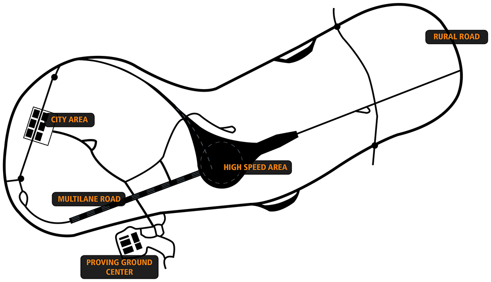
AstaZero proving ground test track showing “rural road” used in this study.

The experiment involved five high-end vehicles, from four different makes, all different models. The system used for trajectory data acquisition was the RT-Range S multiple target ADAS measurements solution by Oxford Technical Solutions, with a differential GPS accuracy. Analysis of the three dimensions (response time, time headway, and stability) was based on the instantaneous positions of the vehicles. Regarding some qualitative characteristics of the campaign, the heading accuracy was around 0.1 degrees, the speed horizontal accuracy around 0.01 m/s, and the horizontal accuracy around 0.02 m. Table 1 shows the basic characteristics of the vehicles, while the same notation is used in the rest of the paper for each vehicle. The first one, VL, is always the leader, while vehicle 2 (V2) is always placed in the middle of the car-platoon (hunter mode in the OXTS software) because of requirements for optimal data acquisition.

Table 1.

Basic Information on Vehicles Used in the Tests

Vehicle	Brand	Engine	Power (kW)
VL (leader)	B3	3L diesel	210
V1	B1	Electric/battery	258
V2	B2	2L diesel	195
V3	B3	3L diesel	210
V4	B4	2L petrol	165

The experiments were organized in laps, where one lap corresponds to the path shown in Figure 1. In all the tests, VL was driven with the ACC enabled to avoid noisy fluctuations around the desired speed because of manual driving. In general, two different car-following patterns were applied for the following vehicles, (a) car-platoon with constant speed and (b) car-platoon with perturbations (deceleration to a new desired speed) from an equilibrium point. For the second pattern, communication between VL and the last follower in the platoon ensured that the speed of the last vehicle was stable at the desired speed and therefore the car-platoon was close to equilibrium prior to applying a new perturbation. When the driver of VL wished to apply a new perturbation, he set the desired speed of the ACC system to a new lower value, the vehicle decelerated using the ACC system, and then the driver reset the desired speed to the previous setting. This procedure was selected to avoid different deceleration patterns on different perturbations and resembles the way that vehicles with ACC enabled behave. For safety reasons in each lap the desired speed was fixed to 13.9–16.7 m/s on the curves and to 25–27.8 m/s on the straight parts.

In the perturbation dataset that is presented in this work the equilibrium speeds were between 16.7 m/s and 27.8 m/s. Furthermore, the perturbation magnitudes were between 2.8 m/s and 13.9 m/s. A summary of the number of detected perturbation events per equilibrium speed and perturbation magnitude is given in Table 2.

Table 2.

Classification of the Perturbations Presented in the Results per Equilibrium Speed and Perturbation Magnitude

Equilibrium speed (m/s) (#number of perturbation events)	Perturbation magnitude (#number of perturbation events)
15–20 m/s (#62)	0–5 m/s (#41)
21–25 m/s (#19)	5–10 m/s (#44)
26–30 m/s (#21)	11–15 m/s (#17)

Data Processing and Methodology

Following the data acquisition, post-processing was performed on the Global Navigation Satellite System (GNSS) and inertial data using the OXTS software and Python scripting for data filtering, subsampling, and segmentation purposes. The response time and time gap study was performed based on the methodology proposed by Makridis et al. ( 24 ).

Response Time

The response time estimations refer to normal (non-critical) driving conditions. In this work, the response time is called observable response time, which is the response that a normal observer would understand under stable and safe conditions. The observable response time has a direct impact on traffic flow. Each response time estimation in this work refers to a specific vehicle and lap. All vehicles drive with their ACC system on and all perturbations were imposed from the controller of VL by lowering the desired speed.

For each lap, the response time for the ACC controller is estimated by correlation between the speed difference of two sequential vehicles and the follower’s acceleration. The idea is based on the assumption that when two vehicles are driven by their ACC controllers under stable car-following conditions, the ACC system of the follower keeps a constant time headway value according to the driver’s desired setting. Under stable conditions, both vehicles ideally have the same speed. At some point in time, VL performs an action that can be either acceleration or deceleration, this action creates a speed difference between the two vehicles and thus changes the time headway of the follower. Since the follower aims to keep a constant time headway, at some later point in time it performs a reaction, which is either acceleration or deceleration, respectively. The time difference between the action of the VL and the response of the follower is defined as the observable response time (response time). In this work, the response time is estimated for each of the four leader-follower pairs of the car-platoon.

In more detail, given the two stationary signals $Δ v_{l - f, t}$ and $a_{f, t}$ , we apply a time delay T on the acceleration of the follower and compute the cross-covariance function between these two signals as follows:

σ_{Δ v, a_{f}} (T) = \frac{1}{N - 1} \sum_{t = 1}^{N} (Δ v_{l - f, t} - μ_{Δ v}) (a_{f, t - T} - μ_{a})

(1)

where $μ_{Δ v}$ and $μ_{a}$ are the means of each time series and N is the number of measurements. The Pearson correlation coefficient which measures the linear correlation between A and B derives from the following normalization:

r_{Δ v, a_{f}} (T) = \frac{σ_{Δ v, a_{f}} (T)}{\sqrt{σ_{Δ v, Δ v} (0) σ_{a_{f}, a_{f}} (0)}}

(2)

where $σ_{Δ v, Δ v} (0) = σ_{Δ v}^{2}$ and $σ_{a_{f}, a_{f}} (0) = σ_{a_{f}}^{2}$ are the variances of each signal. The peak frequency corresponds to the estimated delay, that is, response time for the corresponding test lap. In other words, the response time of the controller is derived by the following:

τ_{delay} = \begin{matrix} argmax (r_{Δ v, a_{f}} (T)) \\ T = {0, 0.1, \dots, T_{\max}} \end{matrix}

(3)

where $T_{\max}$ is the maximum response time assumed in the analysis. In the present work it was assumed that the maximum response time is 4 s. Laps that do not involve perturbations (vehicles driving with constant speed) have low correlation and they are excluded from the results. For this work, results with correlation coefficient value below 0.7 were discarded. For more information, the reader is referred to Makridis et al. ( 24 ).

Time Headway

The time headway is estimated based on laps where all vehicles drive with constant speed and their ACC systems enabled. VL has a constant desired speed and imposes no perturbation. The results were repeated for the maximum and minimum ACC time headway settings.

The instantaneous time gap is computed as follows:

h_{f} (t) = \frac{x_{l} (t) - x_{f} (t)}{v_{f} (t)}

(4)

where $h_{f}$ is the headway, $v_{f} (t)$ is the speed of the follower and $x_{l} (t)$ and $x_{f} (t)$ are the leader’s and follower’s position at time t respectively. For each lap, the desired time gap is estimated by the median value of the instantaneous time gaps:

h_{f, lap} = \tilde{h_{f} (t)}, \forall t \in lap

(5)

The time headway is estimated for all the following vehicles in the car-platoon.

Stability of the Car-Platoon

The speed trajectories are segmented in perturbation events. Each perturbation event is characterized by (a) the equilibrium speed of all the vehicles before the disturbance takes place, and (b) the perturbation magnitude, which is the difference between the minimum speed of the VL during the perturbation and the equilibrium speed of the vehicles before the perturbation. Every perturbation was imposed by lowering the desired speed in the ACC settings of the VL to ensure homogenous behavior during deceleration. In this work, each perturbation event is simplistically characterized by the speed trajectories of all vehicles, ${v_{L} (t), v_{1} (t), v_{2} (t), v_{3} (t), v_{4} (t)}$ , and the perturbation magnitudes which are defined as follows:

m_{V_{i}} = argmax (v_{L} (t)) - argmin (v_{i} (t)) for i \in {L, 1, 2, 3, 4}

(6)

Table 3 summarizes the dataset of empirical measurements used for each of the three dimensions highlighted above.

Table 3.

Summary of the Dataset Generated for all Vehicles Used in the Results

Dimension	Distance (m)	Time (s)	Dataset
Response time	85,326	4,393	72 laps
Time headway	72,158	3,920	24 partial laps
Stability	36,348	1,961	39 perturbations

It should be noted that the stability here is quantified on the basis of each individual perturbation magnitude, while frequency and variation are outside the scope of the present study. Multiple perturbations are not studied together, so the impact of different frequencies is not discussed. Although the acceleration/deceleration patterns during perturbations, as well as the jerk, are parameters that are expected to have a significant impact on traffic flow stability, here, all perturbations are imposed by the ACC controllers and not the human drivers and variation is outside the scope of this work.

Results

This section presents the results along the three main dimensions that can characterize the behavior of an ACC controller: the response time in non-critical conditions, the time headway settings, and the stability of a car-platoon when all vehicles drive with ACC system enabled.

Response Time

In empirical observations, it is clear that the response time is not a crisp value, but rather a distribution of values. This distribution depends on the controller’s logic, the instantaneous conditions during the experiment, and possibly other reasons. Consequently, this study divides the vehicles’ trajectories in laps and provides an estimation of their response time per lap, rather than focusing on finding a unique value per vehicle. There are cases where the correlation of the two signals (speed difference and follower’s acceleration) is low.

Figure 2 illustrates two examples from the correlation procedure. The top subfigures show the two signals, the speed difference (gray), and the acceleration of the follower (black). The middle subfigures show the correlation signal, where the peak corresponds to the maximum correlation position (response time). Finally, the bottom subfigure plots the speed difference signal and the follower’s acceleration, translated for a time equal to the estimated response time. Figure 2a is a successful correlation example. It is clear that the three small perturbations during this lap help the procedure to compute successfully the vehicle’s response time. The correlation coefficient is quite high, 0.86, and the estimated response time has been found equal to 2.5 s. Figure 2b is a discarded lap. The correlation coefficient value is low, 0.63, which means that there is low confidence in the estimated response time. Even visually, it can be observed that both signals are quite steady and no clear correlation between them can be detected. Laps like this one that do not involve perturbations have low correlation and result in unrealistic response times. For this work, results with correlation coefficient values below 0.7 were discarded. The threshold was set in a heuristic way after manual inspection of the results.

Figure 2.

Two examples illustrating the procedure for estimation of response time: (a) high correlation coefficient value and (b) an example with low correlation which was eventually filtered out.

The summary of the response time estimates per vehicles is illustrated in Figure 3. Each point in the scatter plot corresponds to the estimated response time of the vehicle for a distance equal to one lap (around 5.7 km). In total, this work presents the response time of 72 laps (17 for V1, 15 for V2, 19 for V3 and 21 for V4), while 11 laps were discarded because of low correlation coefficient values. Furthermore, for two vehicles (V1 and V2) the correlation seemed to be lower on higher response time estimations. The correlation coefficient value is a measure of trust for the estimation. Consequently, in Figure 3, next to each vehicle there is the weighted response time computed for the specific vehicle over all its laps. The weighted average is computed using the response time weighted by the correlation coefficient, thus results with higher correlation contribute more to the outputted overall response time.

Figure 3.

Estimated response times per vehicle per lap.

It is interesting to note that the vehicle with the electric powertrain, V1, has much faster response times than the rest of the vehicles; it is not clear, however, if the powertrain is related to the lower response times. Moreover, the order of the vehicles in the car-platoon is not constant and no correlation was found between the follower position and the estimated response times. In the future, a more systematic approach needs to be developed to investigate these preliminary findings further. The weighted response time for V1 is 1.7 s, for V2, 2.56 s, for V3, 2.34 s, and for V4, 2.42 s.

Based on the results of the present study, it can be safely assumed that under normal (non-critical) driving car-following conditions the response time can be around 2 s, and this is something that models of ACC systems in microsimulation environments usually do not take into consideration. Consequently, in simulation studies the physical meaning of the ACC system’s response time is lower than the behavior empirically observed. In the literature, the ACC response time parameters take values from the very low order of 0.1–0.2 s ( 10 , 26 ), while other works based on empirical observations, like Milanés and Shladover ( 20 ) and Milanes et al. ( 33 ), confirm that delays were observed in the response of the ACC systems but without providing any quantifiable result. Furthermore, Shladover et al. ( 28 ) highlight the danger of instability in cases of ACC platoons with significant delays in the systems’ reaction, pointing to possible safety-critical issues, which are mentioned also in this work in the stability section.

Time Headway

Time headway results should refer to trajectory parts where the vehicles drive at a constant speed without any deliberately imposed perturbation. Minimal perturbations because of the road geometry and altitude are present, however, as will be discussed later in the section. A visual summary of the results is illustrated in Figure 4. This figure shows the time headway over time per lap per individual vehicle. The notation of the vehicles (V1, V2, V3, V4) is the same as indicated in Table 1 and next to each label there is a number indicating the position of the vehicle in the car-platoon. Furthermore, in parenthesis there is the median time headway per vehicle for the specific trajectory as described by Equation 5. Figure 4, b, c, d, e and f refer to minimum time headway settings for the ACC controllers of the vehicles, while 4a refers to maximum settings. It can inferred that the minimum time headway for the vehicles is a little more than 1 s (1.09–1.36 s) while the maximum value is around 2.5 s, except for V3 for which is around 3.5 s. Furthermore, it seems that the position of the vehicles in the platoon does not play a significant role in the time headway estimations, which are consistent per vehicle across all six laps.

Figure 4.

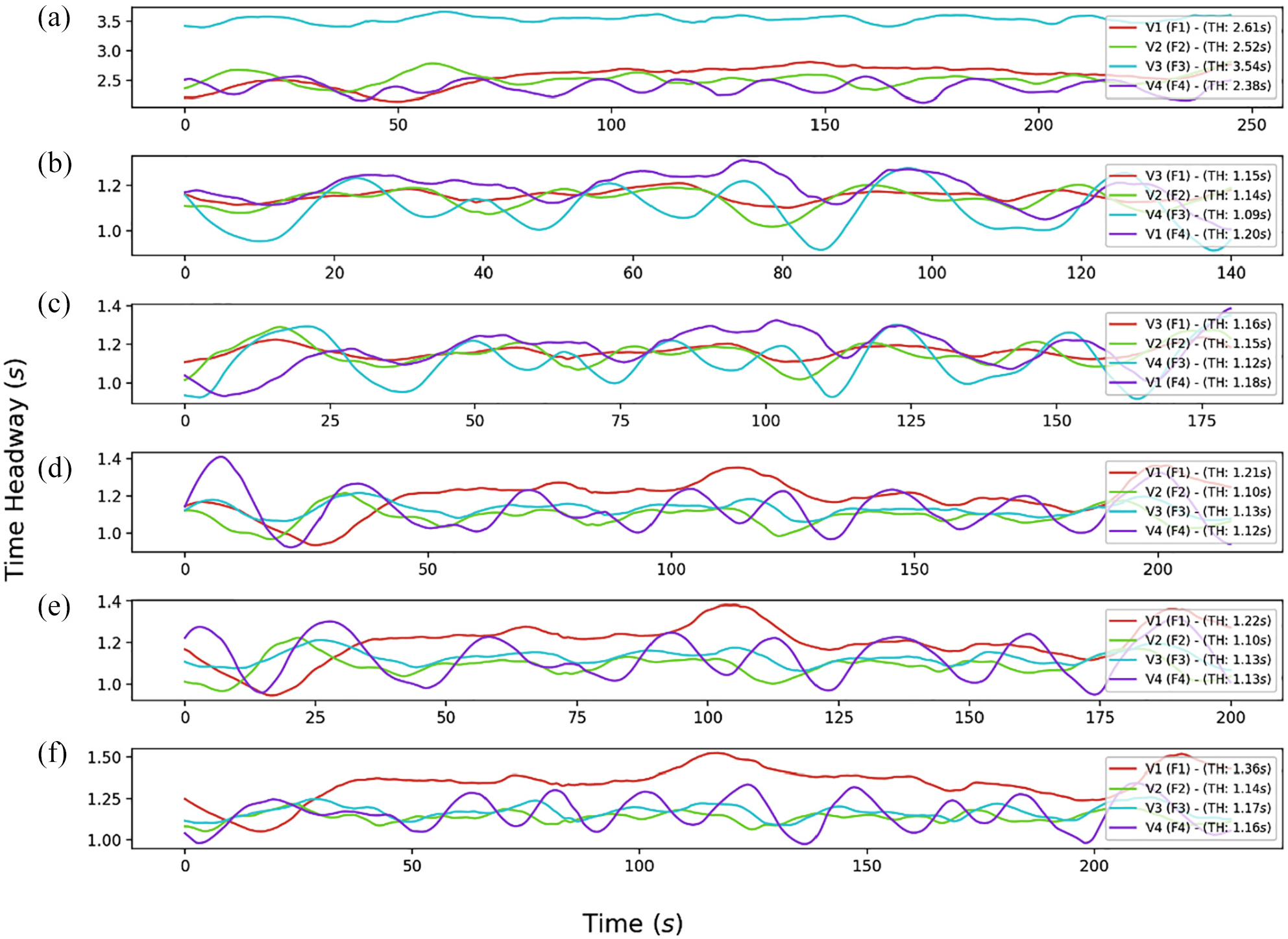
Visual representation of the time headway measurements. (a)-(f) Illustrate for six tests with different vehicle orders, the instantaneous headway measurements for the four following vehicles over time.

Similar to the response time results, based on the above observations, it can be safely assumed that under normal driving car-following conditions the minimum time headway of the vehicles can be around 1.2 s and going up to 2.5 s for V1, V2, and V4 and 3.5 s for V3. The minimum value is closer to the average values considered as parameters for microsimulation modeling of ACC systems. In Ntousakis et al. ( 34 ), it was noticed that the capacity could increase with ACC penetration rate, as long as the time gap setting is less than 1.10–1.20 s. The values found in this study are close to those found empirically in the work of Nowakowski et al. ( 29 ).

Finally, it is worth noting that in Figure 3, the following vehicles towards the end of the car-platoon have significantly higher variation in the time headway than those directly after the VL. Another observation is that the vehicles’ behavior is very similar in Figure 3, d, e , and f where the vehicles are in the same order in the car-platoon and all have the minimum time headway setting, which shows high consistency of the controller over the same path under similar conditions.

String Stability

The last dimension of the results is that concerning string stability of the platoon. Figure 5 presents an overview of the perturbation dataset, which contains 39 perturbation events. Figure 5a shows the magnitude of each perturbation over the speed of the leader when the perturbation started. Most of the events refer to starting speeds between 25 m/s and 27.8 m/s and variable magnitudes from 2.8 m/s to 13.9 m/s for the leading vehicle, VL. Figure 5b compares the perturbation magnitude of the four following vehicles to the magnitude of VL. This graph shows explicitly that for most of the cases the perturbation magnitude grows upstream, up to 7 m/s. More specifically, in all 39 events the magnitude of the first follower is always greater than that of the VL. Next, the magnitude of the second follower is greater than that of the first in 22 events. Interestingly, in 31 events, the magnitude of the third follower is greater than that of the second and finally, in 23 events the magnitude of the fourth follower is greater than that of the third. These patterns show that the car-platoon is instable in all the cases.

Figure 5.

Summary of the perturbation dataset: (a) magnitude of the perturbations over speed and (b) evolution of the perturbation magnitude in the followers in the car-platoon.

Additionally, Figure 6 shows four indicative perturbation events where the instability of the car-platoon is obvious. Each subplot illustrates the speed trajectories of the five vehicles in the car-platoon, while each title displays the magnitude of the perturbation for the leader and the followers. The instability is quite consistent in all the perturbation events but it has been observed that the magnitude for the followers depends on several factors such as the road gradient and curvature, and the vehicles’ order in the car-platoon, and thus the evolution of the perturbation upstream cannot be described in a deterministic way.

Figure 6.

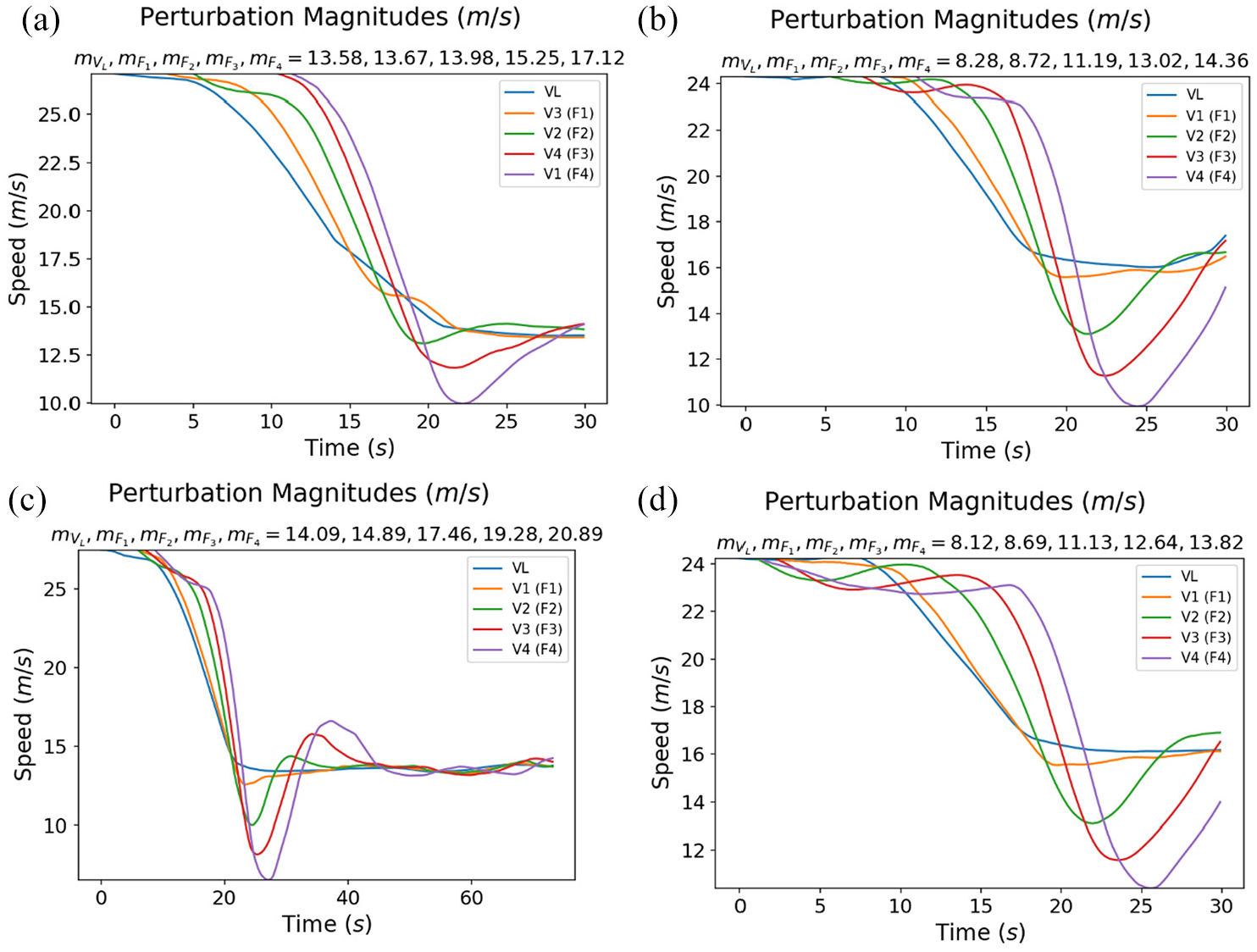
Visual representation of the instability in the car-platoon. (a)–(d) Illustrate four indicative events where the leading vehicle initiates a perturbation. In all figures, the perturbation magnitude of each following vehicle upstream progressively increases.

It is interesting to note that the experimental campaign was designed to study the stability of the car-platoon based on perturbation events of different magnitudes and at various speeds. Before each test, the car-platoon performed a preparatory lap at the desired speed set by the VL to reach a stable condition. In the data post-processing phase, instability was observed during these preparatory laps. Further investigation showed that slight changes in the leader’s speed because of change of the road gradient initiated small perturbations that eventually amplified upstream. In this work, these preliminary findings are presented and the authors plan to investigate further in a structured way the impact of road geometry on the stability of an ACC-controlled car-platoon.

Figure 7 illustrates a time headway trajectory (part of the track), where the ACC controller of the VL was set to a constant desired speed. The controllers of the following vehicles were set to a higher desired speed to perform car-following. The drivers of the five vehicles were only responsible for the steering; there was no intervention on the acceleration of the vehicles. The top figure is the altitude of the rural road of the AstaZero proving ground. The figure in the middle shows the negative correlation (or anticorrelation) between the speed of the VL and the numerical differentiation of the altitude. As the altitude increases, the controller overshoots and the vehicle reaches a speed greater than the desired one, while trying to compensate for the additional work needed because of the increased slope. Similarly, as the altitude decreases, the controller undershoots and the vehicle reaches a speed lower than the desired one. In short, the controller tries to counter-balance the effect of the slope, which eventually leads to oscillations around the desired speed. Finally, the figure at the bottom shows the speed trajectories for all the vehicles in the car-platoon, illustrating how the small oscillation in the speed of the VL affects the four following vehicles. As can be seen, the magnitude of the oscillation of the VL grows as it travels upstream to the followers. More specifically, the (roughly estimated) 1 m/s width of the VL’s speed trajectory grows to 4 m/s for the fifth vehicle in the car-platoon. In a very large car-platoon this instability could theoretically grow to the point that stop-and-go waves could be created by only a slight variation in the gradient of the road. It is also interesting to note that road slope does not always lead to growing perturbations, but this depends on the instantaneous conditions. When the vehicle speed is greater than the desired one (overshooting) and the altitude of the road at that location is increasing, the road slope facilitates the controller to decelerate towards the desired goal speed. Respectively, when the vehicle undershoots and the altitude is decreasing, the road slope facilitates the controller to accelerate towards the desired goal speed.

Figure 7.

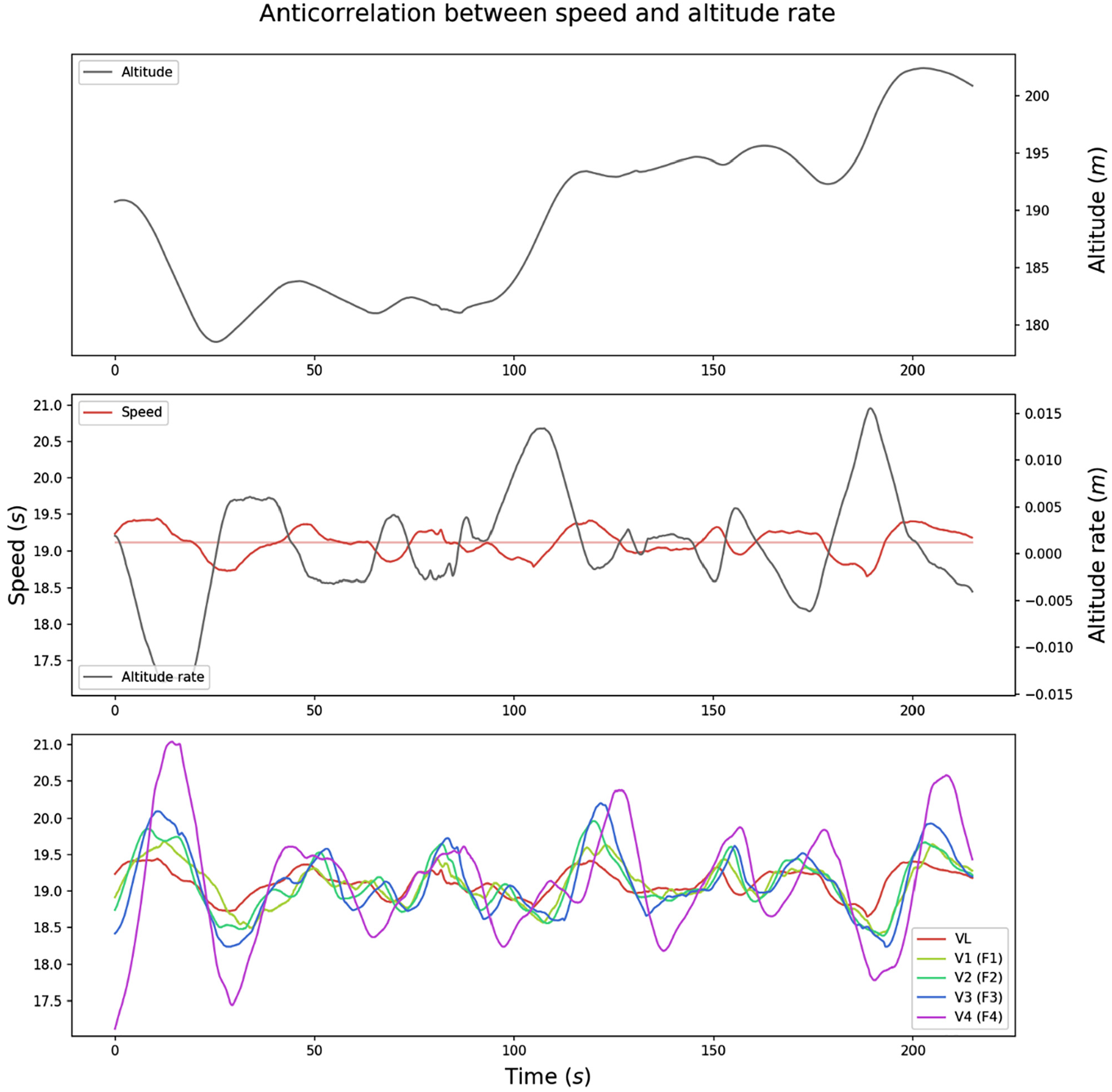
Instability in the car-platoon imposed by change in the road gradient. Top: altitude profile of the rural road test track. Middle: speed of VL and numerical differentiation of the altitude. Bottom: speed trajectories of the five vehicles in the car-platoon.

The speed trajectory parts used to study the instability at a constant desired speed correspond to the partial laps studied in the time headway analysis above. In addition, it is worth mentioning that the conclusions discussed here, based on Figure 7, still hold and remain consistent for all 24 partial laps.

Discussion and Conclusions

Vehicle automation is attracting a great deal of interest in both the market and the research community. The ACC system is the first widely offered automated functionality that regulates the longitudinal movement of the vehicle. As the market penetration of ACC-eq7 vehicles is increasing, so too is the interest in understanding the impact of such controllers in relation to traffic flow, stability, and safety. This is the contribution made by the present paper. This work provides insights on three dimensions of vehicles being driven by their ACC systems: the response time of the controller, available time headway settings, and stability in car-platoons.

An experimental campaign using five commercial vehicle models took place at the proving ground of AstaZero in Sweden. The experimental setup involved car-platoon tests. The leading vehicle (VL), which is always driven by ACC, is followed by four other vehicles (manually or ACC driven). The VL drives either at constant speed or imposes regular perturbations from a speed equilibrium point. The perturbations have different magnitudes to study their impact on the car-platoon stability and understand the response times of the controllers.

Regarding response time estimates, the vehicle with the electric powertrain, V1, showed much faster response times than the others. Moreover, although the sample is not sufficiently large to reach a general conclusion, the responses seem only slighted affected by the position of the following vehicles in the car-platoon The weighted average response time for V1 was found to be 1.7 s, for V2, 2.56 s, for V3, 2.34 s and for V4, 2.42 s.

Time headway was estimated in laps where the desired speed of VL’s ACC was set to a constant value, which became the constant speed of the car-platoon. The minimum time headway for the vehicles was found to be a little more than 1 s (1.09–1.36 s) while the maximum value was around 2.5 s, except for V3 for which it was around 3.5 s. Interestingly, the following vehicles towards the end of the car-platoon had significantly higher variation in the time headway than those directly after the VL.

Furthermore, the driving behavior of each vehicle under similar driving conditions (car-platoon sequence, path, weather, etc.) seems highly auto correlated, which shows high consistency in the decision logic of the controller. Regarding stability, the car-platoon was found to be unstable in all the cases. The instability is visible in all the perturbation events.

Additionally, a correlation was observed between the leader’s speed and the gradient of the road for the laps where the vehicles traveled with constant desired speed. When the altitude increased the controller tried to compensate for the additional work needed because of the increased slope and accelerated, which in most of the cases led to overshooting. When the altitude decreased, the controller again tried to compensate for the extra work produced by the vehicle’s mass and consequently the speed of the vehicle decreased, which in most cases led to undershooting. A small oscillation in the speed of the VL had an effect on the four following vehicles. The magnitude of the oscillation of the VL grows as it travels upstream to the followers. For a very large car-platoon, this instability could theoretically grow to the point of causing stop-and-go waves created only by a slight variation in the slope of the road.

The three dimensions analyzed in this work show different behaviors of the commercially available ACC systems that can affect traffic congestion, traffic safety, passenger comfort, and even energy consumption. Higher response times combined with short time headways ensure better passenger comfort but when the penetration rate of such system increases they are also related to string instability, creating traffic safety concerns. Greater time headways decrease the nominal capacity of the network. Short response times in normal driving conditions can create passenger discomfort. This work raises awareness on the above aspects and shows that the above-mentioned dimensions are interrelated. Manufacturers should ensure that the operation of heterogeneous ACC systems give a priority to traffic safety, while at the same time facilitating traffic flow.

Furthermore, the results of the present work give input to microsimulation studies for a more precise reproduction of ACC dynamics. The string instability observed highlights the need for the design of advanced, string stable controllers. The work of Wilson ( 35 ) is suggested to developers designing linearly string stable controllers. Moreover, the effect of altitude on the ACC speeds showcases the need to develop predictive cruise control that can anticipate changes in the road geometry and respond to multiple leaders, such as in the work of Brugnolli et al. ( 36 ).

The main contributions of the present work to the literature can be summarized as follows:

It conducts a car-platoon test with four following vehicles of different brands with GNSS data acquisition of high accuracy (differential GPS) on a test track under controlled conditions without disturbances from other road users.

It studies simultaneously how four commercial ACC systems function in relation to response time, time headway, and stability.

It provides quantified results on response times and time headway values that can be used in microsimulation modeling of ACC systems.

It highlights the anticorrelation between the road gradient and the speed variation of the leading ACC-enabled vehicle. Weak perturbations caused by the road geometry create instability in the traffic flow, raising concerns about potential consequences when the penetration rate of the ACC systems has increased significantly.

It analyzes empirically the string instability of the car-platoon illustrating quantified results from perturbations of variable magnitudes and at different speeds.

Future work will involve additional experiments with more vehicles and even larger car-platoons to validate further the observations discussed in this work. It will be interesting also to understand whether the behavior of ACC systems changes based on the powertrain of the vehicle. Stability of the car-platoon with manual drivers should be further investigated as well. Additionally, results on the fuel and energy consumption of the vehicles in the car-platoon would be interesting to understand the controllers’ energy efficiency. Finally, a comparison between a human-driven car-platoon and an ACC-driven one in relation to stability, time headway, and response time could be investigated. However, it would be preferable to conduct such tests on road and not on a test track where drivers are usually informed of the experiment and therefore adapt their behavior to the test’s specifications, anticipating perturbations.

Footnotes

Author Contributions

The authors confirm contribution to the paper as follows: study conception and design: M. Makridis, K. Mattas, B. Ciuffo; data collection: M. Makridis, K. Mattas, B. Ciuffo, F. Re, A. Kriston, F. Minarini, G. Rognelund; analysis and interpretation of results: M. Makridis, K. Mattas, B. Ciuffo; draft manuscript preparation: all authors. All authors reviewed the results and approved the final version of the manuscript.

Declaration of Conflicting Interests

The author(s) declared no potential conflicts of interest with respect to the research, authorship, and/or publication of this article.

Funding

The author(s) received no financial support for the research, authorship, and/or publication of this article.

The views expressed in this paper are purely those of the authors and may not, under any circumstances, be regarded as an official position of the European Commission.

References

Publications Office of the European Union. The Future of Road Transport: Implications of Automated, Connected, Low-Carbon and Shared Mobility. https://publications.europa.eu/en/publication-detail/-/publication/67a07945-96f3-11e9-9369-01aa75ed71a1/language-en. Accessed July 22, 2019.

Ciuffo

Zhou

Makridis

Mattas

Yan

Adaptive Cruise Control Strategies Implemented on Experimental Vehicles: A Review. IFAC-PapersOnLine, Vol. 52, No. 5, 2019, pp. 21–27. https://doi.org/10.1016/j.ifacol.2019.09.004.

Davis

L. C.

Multilane Simulations of Traffic Phases. Physical Review E, Vol. 69, No. 1, 2004, p. 016108. https://doi.org/10.1103/PhysRevE.69.016108.

Treiber

Helbing

Microsimulations of Freeway Traffic Including Control Measures. at - Automatisierungstechnik Methoden und Anwendungen der Steuerungs-, Regelungs- und Informationstechnik, Vol. 49, No. 11/2001, 2009, p. 478. https://doi.org/10.1524/auto.2001.49.11.478.

Kesting

Treiber

Schönhof

Kranke

Helbing

Jam-Avoiding Adaptive Cruise Control (ACC) and Its Impact on Traffic Dynamics. In Traffic and Granular Flow ’05 ( Schadschneider

Pöschel

Kühne

Schreckenberg

Wolf

D. E.

, eds.) Springer, Berlin, Heidelberg, 2007, pp. 633–643.

Ioannou

P. A.

Stefanovic

Evaluation of ACC Vehicles in Mixed Traffic: Lane Change Effects and Sensitivity Analysis. IEEE Transactions on Intelligent Transportation Systems, Vol. 6, No. 1, 2005, pp. 79–89. https://doi.org/10.1109/TITS.2005.844226.

Davis

L. C.

Effect of Adaptive Cruise Control Systems on Traffic Flow. Physical Review E, Statistical, Nonlinear, and Soft Matter Physics, Vol. 69, No. 6Pt 2, 2004, p. 066110. https://doi.org/10.1103/PhysRevE.69.066110.

Ford of Europe, Ford Media Center. New Demonstration Shows Ford Driving Tech Can Help Reduce Frustrating Phantom Traffic Jams this Summer. https://media.ford.com/content/fordmedia/feu/en/news/2018/07/18/new-demonstration-shows-ford-driving-tech-can-help-reduce-frustr.html. Accessed July 22, 2019.

Zhu

Gonder

Bjarkvik

Pourabdollah

Lindenberg

An Automated Vehicle Fuel Economy Benefits Evaluation Framework Using Real-World Travel and Traffic Data. IEEE Intelligent Transportation Systems Magazine, Vol. 11, No. 3, 2019, pp. 29–41. https://doi.org/10.1109/MITS.2019.2919537.

10.

Kesting

Treiber

Schönhof

Helbing

Adaptive Cruise Control Design for Active Congestion Avoidance. Transportation Research Part C: Emerging Technologies, Vol. 16, No. 6, 2008, pp. 668–683. https://doi.org/10.1016/j.trc.2007.12.004.

11.

Xiao

Gao

A Comprehensive Review of the Development of Adaptive Cruise Control Systems. Vehicle System Dynamics, Vol. 48, No. 10, 2010, pp. 1167–1192. https://doi.org/10.1080/00423110903365910.

12.

Wagner

Impacts of Gradual Automated Vehicle Penetration on Motorway Operation: A Comprehensive Evaluation. European Transport Research Review, Vol. 11, No. 1, 2019, p. 36. https://doi.org/10.1186/s12544-019-0375-3.

13.

Mattas

Makridis

Hallac

Raposo

M. A.

Thiel

Toledo

Ciuffo

Simulating Deployment of Connectivity and Automation on the Antwerp Ring Road. IET Intelligent Transport Systems, Vol. 12, No. 9, 2018, pp. 1036–1044. https://doi.org/10.1049/iet-its.2018.5287.

14.

Shladover

S. E.

X. Y.

Impacts of Cooperative Adaptive Cruise Control on Freeway Traffic Flow. Transportation Research Record: Journal of the Transportation Research Board, 2012. 2324: 63–70.

15.

Wilson

R. E.

Ward

J. A.

Car-Following Models: Fifty Years of Linear Stability Analysis – a Mathematical Perspective. Transportation Planning and Technology, Vol. 34, No. 1, 2011, pp. 3–18. https://doi.org/10.1080/03081060.2011.530826.

16.

Sun

Zheng

Sun

Stability Analysis Methods and Their Applicability to Car-Following Models in Conventional and Connected Environments. Transportation Research Part B: Methodological, Vol. 109, 2018, pp. 212–237. https://doi.org/10.1016/j.trb.2018.01.013.

17.

Wang

Zhang

Influence of Driving Behaviors on the Stability in Car Following. IEEE Transactions on Intelligent Transportation Systems, Vol. 20, No. 3, 2019, pp. 1081–1098. https://doi.org/10.1109/TITS.2018.2837740.

18.

Wang

Longitudinal Safety Impacts of Cooperative Adaptive Cruise Control Vehicle’s Degradation. Journal of Safety Research, Vol. 69, 2019, pp. 177–192. https://doi.org/10.1016/j.jsr.2019.03.002.

19.

Han

Sciarretta

Ojeda

L. L.

Nunzio

G. D.

Thibault

Safe- and Eco-Driving Control for Connected and Automated Electric Vehicles Using Analytical State-Constrained Optimal Solution. IEEE Transactions on Intelligent Vehicles, Vol. 3, No. 2, 2018, pp. 163–172. https://doi.org/10.1109/TIV.2018.2804162.

20.

Milanés

Shladover

S. E.

Modeling Cooperative and Autonomous Adaptive Cruise Control Dynamic Responses Using Experimental Data. Transportation Research Part C: Emerging Technologies, Vol. 48, No. Supplement C, 2014, pp. 285–300. https://doi.org/10.1016/j.trc.2014.09.001.

21.

Shladover

S. E.

Connected and Automated Vehicle Systems: Introduction and Overview. Journal of Intelligent Transportation Systems, Vol. 22, No. 3, 2018, pp. 190–200. https://doi.org/10.1080/15472450.2017.1336053.

22.

Knoop

V. L.

Wang

Wilmink

Hoedemaeker

D. M.

Maaskant

Van der Meer

E. J.

Platoon of SAE Level-2 Automated Vehicles on Public Roads: Setup, Traffic Interactions, and Stability. Transportation Research Record: Journal of the Transportation Research Board, 2019. 2673: 311–322.

23.

Gunter

Gloudemans

Stern

R. E.

McQuade

Bhadani

Bunting

Monache

M. L. D.

Lysecky

Seibold

Sprinkle

Piccoli

Work

D. B.

Are Commercially Implemented Adaptive Cruise Control Systems String Stable?

arXiv Preprint arXiv:1905.02108 [cs], 2019.

24.

Makridis

Mattas

Ciuffo

Response Time and Time Headway of an Adaptive Cruise Control. An Empirical Characterization and Potential Impacts on Road Capacity. IEEE Transactions on Intelligent Transportation Systems, 2019, pp. 1–10. https://doi.org/10.1109/TITS.2019.2948646.

25.

Makridis

Mattas

Borio

Ciuffo

Estimating Empirically the Response Time of Commercially Available ACC Controllers Under Urban and Freeway Conditions. Proc., 2019 6th International Conference on Models and Technologies for Intelligent Transportation Systems, Cracow, Poland, 2019.

26.

Green

“How Long Does It Take to Stop?” Methodological Analysis of Driver Perception-Brake Times. Transportation Human Factors, Vol. 2, No. 3, 2000, pp. 195–216. https://doi.org/10.1207/STHF0203_1.

27.

Zhu

Wang

Impact on Car Following Behavior of a Forward Collision Warning System with Headway Monitoring. Transportation Research Part C: Emerging Technologies, Vol. 111, 2020, pp. 226–244. https://doi.org/10.1016/j.trc.2019.12.015.

28.

Shladover

S. E.

Nowakowski

X.-Y.

Ferlis

Cooperative Adaptive Cruise Control: Definitions and Operating Concepts. Transportation Research Record: Journal of the Transportation Research Board, 2015. 2489: 145–152.

29.

Nowakowski

O’Connell

Shladover

S. E.

Cody

Cooperative Adaptive Cruise Control: Driver Acceptance of Following Gap Settings Less than One Second. Proceedings of the Human Factors and Ergonomics Society Annual Meeting, Vol. 54, No. 24, 2010, pp. 2033–2037. https://doi.org/10.1177/154193121005402403.

30.

Patel

Levin

M. W.

Boyles

S. D.

Effects of Autonomous Vehicle Behavior on Arterial and Freeway Networks. Transportation Research Record: Journal of the Transportation Research Board, 2016. 2561: 9–17.

31.

Calvert

S. C.

van den Broek

T. H. A.

van Noort

Cooperative Driving in Mixed Traffic Networks #x2014; Optimizing for Performance. Proc., 2012 IEEE Intelligent Vehicles Symposium, Alcala de Henares, Spain, 2012.

32.

Wang

Daamen

Hoogendoorn

Arem

B. V.

Potential Impacts of Ecological Adaptive Cruise Control Systems on Traffic and Environment. IET Intelligent Transport Systems, Vol. 8, No. 2, 2014, pp. 77–86. https://doi.org/10.1049/iet-its.2012.0069.

33.

Milanes

Shladover

S. E.

Spring

Nowakowski

Kawazoe

Nakamura

Cooperative Adaptive Cruise Control in Real Traffic Situations. IEEE Transactions on Intelligent Transportation Systems, Vol. 15, No. 1, 2014, pp. 296–305. https://doi.org/10.1109/TITS.2013.2278494.

34.

Ntousakis

I. A.

Nikolos

I. K.

Papageorgiou

On Microscopic Modelling of Adaptive Cruise Control Systems. Transportation Research Procedia, Vol. 6, No. Supplement C, 2015, pp. 111–127. https://doi.org/10.1016/j.trpro.2015.03.010.

35.

Wilson

R. E.

Mechanisms for Spatio-Temporal Pattern Formation in Highway Traffic Models. Philosophical Transactions. Series A, Mathematical, Physical, and Engineering Sciences, Vol. 366, No. 1872, 2008, pp. 2017–2032. https://doi.org/10.1098/rsta.2008.0018.

36.

Brugnolli

M. M.

Angélico

B. A.

Laganá

A. A. M.

Predictive Adaptive Cruise Control Using a Customized ECU. IEEE Access, Vol. 7, 2019, pp. 55305–55317. https://doi.org/10.1109/ACCESS.2019.2907011.