Sage Journals: Discover world-class research

Abstract

Cooperative (automated) vehicles have the potential to enhance traffic efficiency and fuel economy on urban roads, especially at signalized intersections. An optimal control approach to optimize the trajectories of cooperative vehicles at fixed-timing signalized intersections along an arterial is presented. The proposed approach aims to optimize throughput first, and then to maximize comfort while minimizing travel delay and fuel consumption. The proposed approach is flexible in dealing with both quadratic and more complex cost functions. Assuming fixed timing signal control in a cycle and vehicle-to-infrastructure communication, the red phase is taken into account in position constraints for vehicles that cannot pass the intersection in the green phase. Safety is guaranteed by constraining the inter-vehicle distance larger than some desired value. The approach is scalable and can be used for joint trajectory planning of one platoon approaching another stationary platoon. It can also be extended to multiple intersections with fixed signal plans. To verify the performances of the controlled platoon, simulation under three different traffic scenarios is conducted, namely: an isolated intersection with/without downstream vehicle queues, and platoon control at multiple intersections. Three baseline scenarios without control are also designed to compare performances in relation to both mobility and fuel consumption in each controlled scenario. The results demonstrate that the controlled vehicles generate plausible behavior under control objectives and constraints. Moreover, the consideration of downstream vehicle queues and the application at both an isolated signalized intersection and arterial corridors on urban roads verify the flexible characteristics of the control framework.

From the perspective of safety, setting traffic lights on urban roads is an important traffic control approach ( 1 ). At signalized intersections, vehicles have to stop during the red phase and restart when the green phase starts. Therefore, vehicles are always accelerating and decelerating, and even stopping, in the vicinity of signalized intersections, which results in traffic shock waves, and causes travel delay as well as excessive fuel consumption and emissions ( 2 ). With the development of cyber-physical technologies, connected and automated vehicles (CAVs) are able to extend the sensing and anticipation range when approaching signalized intersections, and to coordinate their decisions for a common goal ( 3 ). CAVs have the potential to improve efficiency, safety, and sustainability at signalized intersections. Thus, it is desirable to take advantage of CAV technologies for effective traffic operations at signalized intersections.

Significant research efforts have focused on CAV platooning on highways ( 4 – 7 ), however, less attention has been devoted to the design of CAV platoons on urban roads. Vehicle acceleration/deceleration maneuvers in the vicinity of signalized intersections on urban roads produce high levels of emissions and fuel consumption, in addition to travel delays ( 8 ). Thus it is valuable to optimize the fuel efficiency of vehicles at signalized intersections. Many existing research efforts on optimization-based control framework design on urban roads have applied different microscopic fuel consumption models ( 9 – 11 ) in simulations to validate their effectiveness in reducing fuel consumption and emission and/or delay (average stop time) ( 12 – 16 ). These were only simulated at isolated intersections, however. Neither energy consumption nor the combined optimization of fuel efficiency and travel delay was designed in the objective function, which could actually reflect the realistic performance of the controlled vehicles.

The literature on trajectory control of CAV systems can be grouped into two categories: vehicle-to-vehicle (V2V)-based trajectory control and vehicle-to-infrastructre (V2I)-based speed advice/control. As to V2V-based trajectory control, several control algorithms have been proposed at an isolated intersection without a traffic signal. Some researchers have argued that the application of CAV technologies to traffic control has the potential to remove traditional signal controllers at isolated intersections, if reliable connectivity of V2V information was provided ( 17 – 20 ). Such proposed control algorithms were designed with the aim of avoiding collisions and improving traffic efficiency, that is, in reduced travel time and total delay. These control algorithms could not account for potential conflicts and safety problems of pedestrian and bicyclists, however, and they were confined to an isolated intersection. These two features rendered these algorithms far away from realistic traffic operations.

As to V2I-based speed advice systems, a number of efforts have been made to investigate optimization-based speed advice algorithms on urban arterials via V2I communication. Some optimization-based velocity planning algorithms used simplified objective functions, such as maximizing the absolute value of accelerations or minimizing the differences between actual and maximum feasible speeds, when safety constraints were satisfied ( 21 – 23 ). A green-light optimized speed advisory (GLOSA) system was proposed to provide drivers with speed advice on urban corridors by calculating travel time to the stop-line ( 24 – 26 ) or by minimizing fuel consumption ( 27 – 29 ) or delay ( 28 ). However, such speed advice systems which were designed for signalized intersections could only consider one criterion in the objective function, ignoring the comprehensive traffic operations in reality.

A few speed advisory or optimization systems have been designed under actuated or adaptive signal control approaches. As to the actuated signal control approach (without optimizing signal parameters), speed advisory systems were designed at isolated actuated signalized intersections ( 2 , 30 ) or corridors with actuated signal traffic lights ( 31 ). An optimization-based speed control algorithm was proposed on arterials by combining the control effects of isolated intersections ( 32 ). With respect to the integrated optimization of adaptive traffic signals and vehicle trajectories, existing research efforts mainly focused on isolated intersections ( 33 , 34 ). However, only acceleration fluctuations of platoon leaders were optimized over time as representative of energy savings and emission reductions of the whole platoon, which could not be extended to accurately reveal optimal eco-driving performances of the whole platoon. In addition, actuated or adaptive signal control approaches will add computational complexity to an optimization-based control approach. Thus, the present study designs a control system under a fixed-timing control approach, which only requires fixed-timing cycles within the prediction horizon.

From the discussion above, it may be concluded that the existing control algorithms are not able to optimize both fuel efficiency and travel delay for the whole platoon. In addition, it is not evident that the existing algorithms are scalable to multiple intersections. This paper aims to design an optimal platoon trajectory control method by optimizing accelerations of the controlled CAV platoon when satisfying safe driving requirements. The proposed control approach obtains the optimal throughput first, and then maximizes driving comfort (by minimizing accelerations) and simultaneously minimizes average travel delay (by maximizing vehicle speeds) and fuel consumption rates, subject to admissible constraints on acceleration and speed. Rear-end collisions are avoided by constraining the inter-vehicle distance to be greater than the (minimum) safe gap. The red phase is formulated as a position constraint for vehicles that cannot pass the stop-line during the green phase. The control approach is flexible in incorporating queue discharging features on intersection approaches, as well as the platoon splitting and merging performances. Thus, the proposed framework is flexible in that it could be applied at multiple intersections with queues on signalized intersection approaches under multiple criteria in the objective function. These criteria could be applied to any controlled vehicle at any time step within the prediction horizon. Finally, the performance of the proposed control method is verified by simulation using several scenarios.

The remainder of the paper is organized as follows: The following section introduces the control formulation for longitudinal driving task, followed by analysis of the simulation results. The study is summarized in the final section.

Control Formulation

The longitudinal platoon control problem is formulated in this section, including design assumptions, control objectives and constraints, system dynamics, and solution approach.

Design Assumptions and Description of the Control Problem

The basic assumptions in this optimal trajectory design are described as follows:

Fixed signal timing during a cycle at signalized intersections;

Signal plan communicated to CAVs via infrastructure-to-vehicle (I2V) communication;

CAVs with V2V, V2I between signal controllers;

Acceleration of CAVs controlled;

Low or medium traffic demand without spillback.

An environment with 100% CAVs is considered, to demonstrate the workings of the proposed approach. First, let us consider the simplest scenario, that is, an isolated intersection without a queue. The longitudinal position of the stop-line is defined as 0. When the leader of CAV platoon reaches L₀ meters upstream of the stop-line, the platoon trajectory optimization starts. The prediction horizon T is regarded to start from the time when the leader of the driving platoon arrives at a point L₀ meters away from the stop-line to the end of this cycle, including at least one green phase and one red phase. Assuming that the signal indication is green when the optimization starts, the prediction horizon could be described as T = g₁+r. g₁ and r are defined as the length of the remaining green phase and red phase in the current cycle when control starts, respectively. The control problem is to optimize acceleration trajectories to fulfill multiple control objectives and constraints, which will be detailed in the following subsections.

More complex scenarios occur when downstream vehicle queues are taken into account on urban corridors. As shown in Figure 1, a driving platoon is traveling along the corridor when downstream CAVs are queuing before the stop-lines. The driving platoon can be treated in the same way as in the isolated intersection scenario. L₁ denotes the lane length between the stop-lines of the upstream and the adjacent downstream (second) intersection. The prediction horizon T is considered to start from the time when the leader of the driving platoon arrives L₀ meters away from the stop-line in the upstream direction at the first intersection to the green phase at the second intersection ends.

Figure 1.

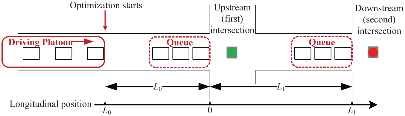
Illustration of operation of the control system.

Control Objectives

Because of the red phase, the platoon may be split into two parts in the control design. The first part of the driving platoon is required to operate with minimum travel delay, passing the first intersection (i.e., the intersection farthest upstream) as soon as possible. Meanwhile, the maximum number of vehicles that could depart from the first upstream intersection is one of the variables that could be optimized. On the other hand, the second part of the driving platoon consists of vehicles that will find it impossible to leave the intersection. Thus, they are expected to operate with minimum energy consumption and emissions, stop in front of the stop-line during the red phase, and restart at the beginning of the green phase. Furthermore, driving comfort and safety requirements of the whole platoon are considered. All these strategies make sure that the controlled platoon is able to operate efficiently.

The control design is expected to fulfill the following objectives:

To maximize driving comfort (by minimizing accelerations);

To minimize the travel delay of passing vehicles (by maximizing vehicle speeds);

To maximize the number of vehicles able to pass the stop-lines during the (remaining) green phases;

To minimize the fuel consumption of vehicles that could not pass the stop-line during the remaining green phase and the following red phase.

In addition, the controller should satisfy the no-collision driving requirement.

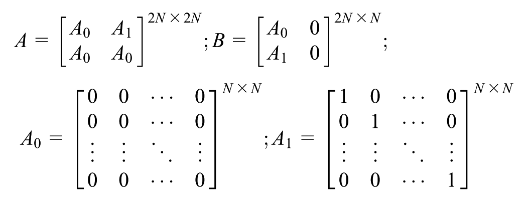
System Dynamics Model

The control input variable u is the acceleration, a_i(t), and the maximum number of vehicles q (veh) that could pass the stop-line; i denotes the vehicle sequence number on a single lane, and N is the number of controlled vehicles. State variables x are considered as the longitudinal position, x_i(t), and the speed, v_i(t), of the controlled vehicle i. x_i(t)⩾0 implies vehicle i passes the stop-line at the most upstream intersection, while x_i(t)<0 means it is still on the approach ahead of the stop-line at the most upstream intersection.

\begin{matrix} x = {(x_{1} (t), . . ., x_{i} (t), . . ., x_{N} (t), v_{1} (t), . . ., v_{i} (t), . . ., v_{N} (t))}^{T} \\ u = {(a_{1} (t), . . ., a_{i} (t), . . ., a_{N} (t))}^{T} \end{matrix}

(1)

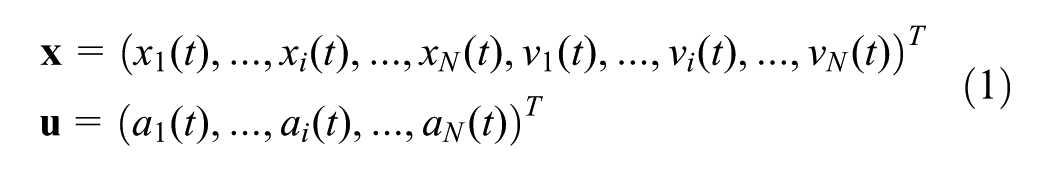
The longitudinal dynamics model is described by the following ordinary differential equation:

\frac{d}{d t} x = \frac{d}{d t} {(x_{1} (t), . . ., x_{i} (t), . . ., x_{N} (t), v_{1} (t), . . ., v_{i} (t), . . ., v_{N} (t))}^{T} = f (x, u)

(2)

f (x, u) = A x + B u

(3)

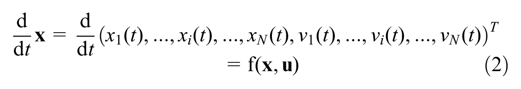
where

A = {[\begin{matrix} A_{0} & A_{1} \\ A_{0} & A_{0} \end{matrix}]}^{2 N \times 2 N}; B = {[\begin{matrix} A_{0} & 0 \\ A_{1} & 0 \end{matrix}]}^{2 N \times N}; A_{0} = {[\begin{matrix} 0 & 0 & \dots & 0 \\ 0 & 0 & \dots & 0 \\ ⋮ & ⋮ & ⋱ & ⋮ \\ 0 & 0 & \dots & 0 \end{matrix}]}^{N \times N}; A_{1} = {[\begin{matrix} 1 & 0 & \dots & 0 \\ 0 & 1 & \dots & 0 \\ ⋮ & ⋮ & ⋱ & ⋮ \\ 0 & 0 & \dots & 1 \end{matrix}]}^{N \times N}

Optimal Control Problem Formulation

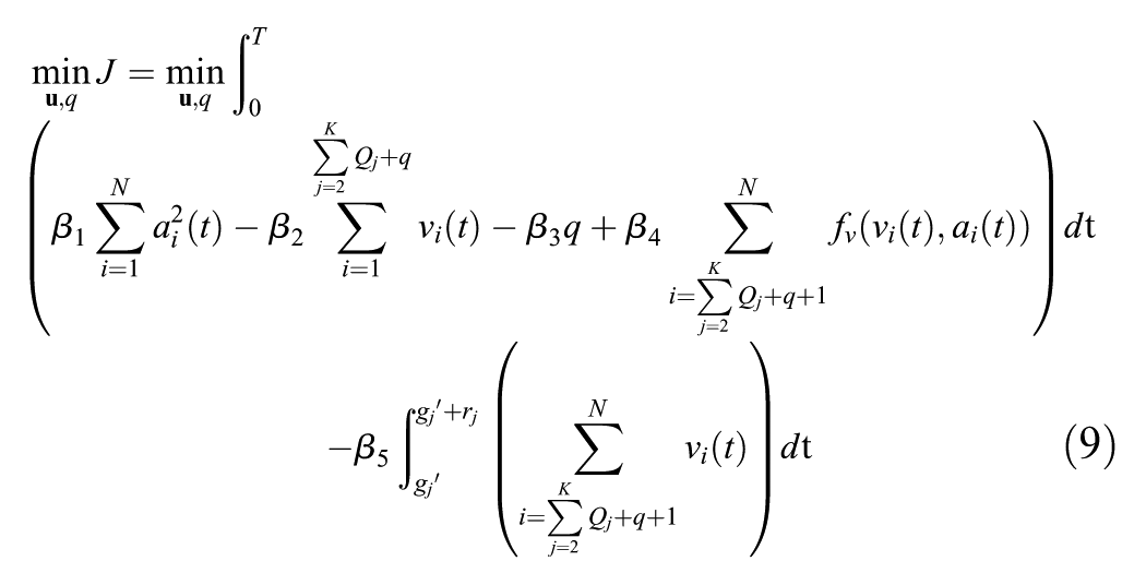
From the above discussion, the formulation of the control problem at an isolated signalized intersection without a queue could be described as:

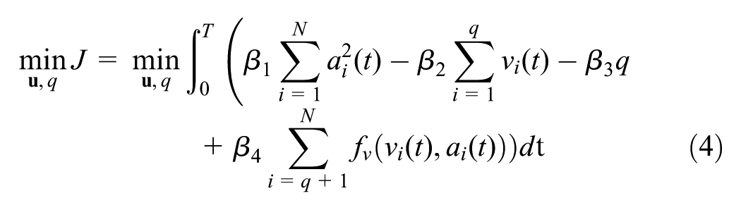
\min_{u, q} J = \min_{u, q} \int_{0}^{T} (β_{1} \sum_{i = 1}^{N} a_{i}^{2} (t) - β_{2} \sum_{i = 1}^{q} v_{i} (t) - β_{3} q + β_{4} \sum_{i = q + 1}^{N} f_{v} (v_{i} (t), a_{i} (t))) d t

(4)

Here, β₁, β₂, β₃, and β₄ are cost weights; f_v is the instantaneous fuel consumption rate which could capture transient changes in speed and acceleration. For typical vehicles on a flat road, the instantaneous fuel consumption rate f_v (ml/s) in Equation 4 could be estimated as

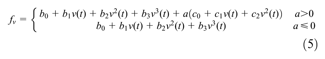
f_{v} = {\begin{matrix} b_{0} + b_{1} v (t) + b_{2} v^{2} (t) + b_{3} v^{3} (t) + a (c_{0} + c_{1} v (t) + c_{2} v^{2} (t)) & a > 0 \\ b_{0} + b_{1} v (t) + b_{2} v^{2} (t) + b_{3} v^{3} (t) & a ⩽ 0 \end{matrix}

(5)

Detailed parameter values can be found in Kamal et al. ( 12 ). Optimizing instantaneous consumption rates may give the trivial optimal solution of v=0 and a=0, but this problem is overcome by maximizing speeds in the objective function.

In Equation 4, the passing q vehicles are optimized to depart in maximal speeds while vehicles that could not dissipate are expected to operate with minimum fuel consumption rates. In addition, driving comfort for all controlled vehicles is included, as shown in the first cost term of Equation 4. Note that q is a variable which also needs to be optimized. An upper bound is defined for the maximum passing vehicle number in the remaining green time, M₁. M₁ could be obtained as follows

M_{1} = ceil (\frac{g_{1} - L_{0} / v_{\max}}{t_{\min}})

(6)

where v_max denotes the limit speed on a single lane with signalized intersections and t_min denotes the minimum safe car-following time gap. All the integer values that are not more than M₁ are given to q (q⩽M₁), thus q is a constant in the objective function. Based on the enumeration of possible q, the biggest value of q is selected in the condition that all these q vehicles could pass the stop-line during the green phase. In this way, q is optimized, and then the objective function is minimized with this optimal q value. Although the objective function value will decline with an increase in q value, q is limited by the signal status. There is a position constraint for these q vehicles when the signal status turns red, which means that it is mandatory for them to pass the intersection during the green phase.

The aforementioned formulation can be extended to capture features of queues and multiple intersections on the arterial if the isolated signalized intersection is regarded as the first upstream intersection. The joint control of multiple intersections along a corridor is different from combining the control of isolated intersections because of the different objective function during the prediction horizon, which is detailed in Equation 7. The formulation of the control problem regarding two intersections with queues could be described as:

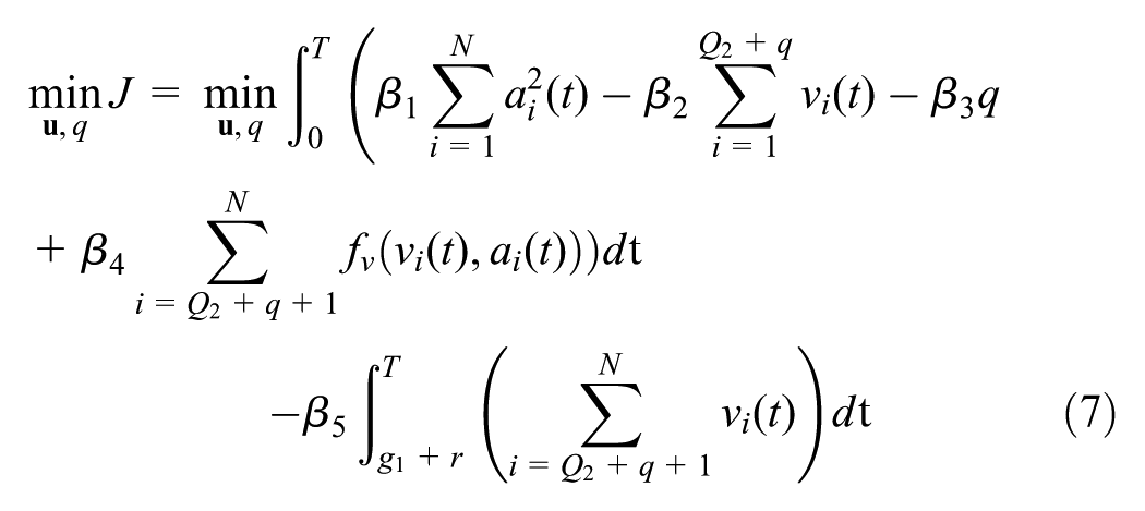
\min_{u, q} J = \min_{u, q} \int_{0}^{T} (β_{1} \sum_{i = 1}^{N} a_{i}^{2} (t) - β_{2} \sum_{i = 1}^{Q_{2} + q} v_{i} (t) - β_{3} q + β_{4} \sum_{i = Q_{2} + q + 1}^{N} f_{v} (v_{i} (t), a_{i} (t))) d t - β_{5} \int_{g_{1} + r}^{T} (\sum_{i = Q_{2} + q + 1}^{N} v_{i} (t)) d t

(7)

where N is the number of vehicles in the controlled platoon, including the driving platoon and the vehicles queued at intersections; q could be regarded as the maximum number of vehicles that could pass the stop-line at the most upstream intersection; and Q₂ denotes the number of vehicles in the downstream vehicle queues. Assuming that the traffic demand on the corridor is not very high, the Q₂ and q vehicles are supposed to discharge during the green phases along the corridor. If i denotes the vehicle sequence number in a single lane (i⩾0), then vehicles between i = 1 and i = Q₂ are regarded as the vehicle queues on the downstream intersection approaches, and the vehicle sequence number of the q passing vehicles at the most upstream intersection is therefore described as i = Q₂+ 1 to i = Q₂+q. g₁ and r are defined as the length of the remaining green phase and the red phase in the current cycle at the most upstream intersection when control starts. In Equation 7, the passing q vehicles and Q₂ vehicles in the downstream queues are optimized to depart at maximal speeds within the whole prediction horizon, while vehicles that could not dissipate at the most upstream intersection are expected to operate with minimum fuel consumption rates. Driving comfort is considered in all controlled vehicles. In addition, the fifth cost term shows that the vehicles that could not depart at the most upstream intersection are instructed to maximize their speeds when the signal indication turns green in the next cycle at the most upstream intersection. The maximum passing vehicle number in the remaining green time at the most upstream intersection considering queue, M, could be obtained as follows

M = ceil (\frac{g_{1} - L_{0} / v_{\max}}{t_{\min}}) + Q_{1}

(8)

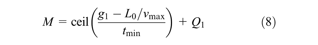
Q ₁ denotes the downstream vehicle queue at the most upstream intersection. It should be noted that the optimal value of q could be obtained based on M, which is similar, as discussed in Equation 6.

Similarly, the generic control problem formulation regarding multiple intersections with queues could be described as:

\begin{matrix} \min_{u, q} J = \min_{u, q} \int_{0}^{T} (β_{1} \sum_{i = 1}^{N} a_{i}^{2} (t) - β_{2} \sum_{i = 1}^{\sum_{j = 2}^{K} Q_{j} + q} v_{i} (t) - β_{3} q + β_{4} \sum_{i = \sum_{j = 2}^{K} Q_{j} + q + 1}^{N} f_{v} (v_{i} (t), a_{i} (t))) d t \\ - β_{5} \int_{g_{j}'}^{g_{j}' + r_{j}} (\sum_{i = \sum_{j = 2}^{K} Q_{j} + q + 1}^{N} v_{i} (t)) d t \end{matrix}

(9)

Assuming that the most upstream intersection is the first intersection, j (j⩾2) denotes the downstream intersection sequence along the corridor, and K is the number of intersections that the controlled platoon will pass within the prediction horizon. Here, Q_j means the sequence number of vehicle queue at the jth intersection, g_j represents the moment when the signal indication turns red at the jth intersection, and r_j is the length of the red phase at the jth intersection.

Controller Constraints

The control problem requires the control and state variables to respect some constraints:

Admissible acceleration is bounded between maximum acceleration, a_max, and minimum acceleration, a_min.

a_{\min} ⩽ a_{i} (t) ⩽ a_{\max}

(10)

2. Speed is restricted to be no larger than the limit speed, v_max, but non-negative.

0 ⩽ v_{i} (t) ⩽ v_{\max}

(11)

3. No-collision requirements: space gap and time gap is required to be greater than or equal to the minimum safe gap within the prediction horizon.

x_{i} (t) - x_{i + 1} (t) ⩾ v_{i + 1} (t) t_{\min} + s_{0} + l

(12)

l denotes the length of a standard vehicle and s₀ is the minimum space gap in stationary conditions.

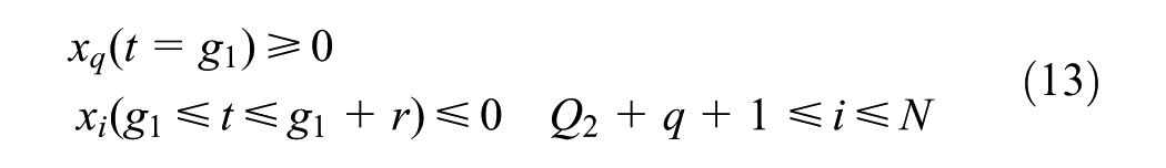
4. Red phase position constraint

The red phases within the prediction horizon are regarded as position constraints, which could adapt to deal with queues by adjusting the value of Q₂ and signal timing parameters g₁ and r at the most upstream intersection. There are two position constraints regarding the red phase. Taking the simple scenario of two intersections along a corridor as an example, the qth vehicle should be restricted to pass the stop-line during the green phase at the most upstream intersection after optimizing the value of q, that is, the longitudinal position of the qth vehicle should be greater than or equal to 0 at the end of green phase at the first intersection. In addition, the i = Q₂+q+ 1 to i = N vehicles which will encounter the red phase at the most upstream intersection should be constrained to stop behind the stop-line during the red phase, which means that the longitudinal positions of i = Q₂+q+ 1 to i = N vehicles should be less than or equal to 0 during the red phase at the first intersection. These constraints could be expressed as follows:

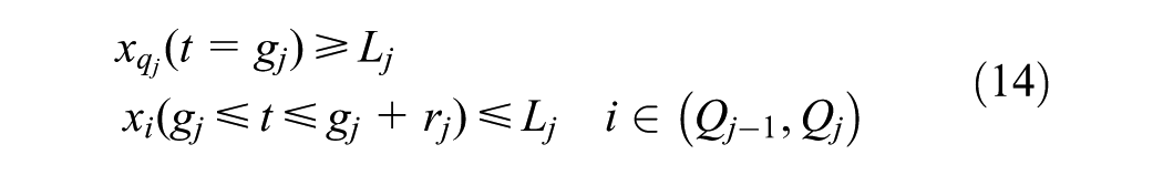
\begin{matrix} x_{q} (t = g_{1}) ⩾ 0 \\ \begin{matrix} x_{i} (g_{1} ⩽ t ⩽ g_{1} + r) ⩽ 0 & Q_{2} + q + 1 \end{matrix} ⩽ i ⩽ N \end{matrix}

(13)

The position constraints can also be applied at multiple intersections along the corridor. Here, L_j is defined as the longitudinal position of the stop-line at the jth intersection. If q_j denotes the optimal number of passing vehicles at the jth intersection in the controlled platoon sequence, then the longitudinal position of q_j should be greater than or equal to L_j when the signal turns red at the jth intersection. In addition, the vehicle queue at the jth intersection, Q_j, should be restricted to stop behind the stop-line during the red phase at the jth intersection, as shown in Equation 14.

\begin{matrix} x_{q_{j}} (t = g_{j}) ⩾ L_{j} \\ \begin{matrix} x_{i} (g_{j} ⩽ t ⩽ g_{j} + r_{j}) ⩽ L_{j} & i \in (Q_{j - 1}, Q_{j}) \end{matrix} \end{matrix}

(14)

Solution Approach

The continuous-time optimal control problem is transformed into a nonlinear programming (NLP) problem by discretizing the control variable of accelerations within the prediction horizon. System dynamics are transcribed as linear equality constraints in the NLP problem. The linear inequality constraints on the control variable, that is, lower and upper bounds on acceleration, are set to limit the admissible control signals. Other linear inequality constraints regarding speed, safe gap, and longitudinal position during the red phase are described in the form of control variables using the system dynamic equation, as the solver required. Thus, every vehicle in the controlled platoon at every moment within the prediction horizon obeys all constraints in the controller. This optimal control problem is solved with the fmincon function in the MATLAB environment, using the SQP algorithm. The performance of the controller is discussed in the next section.

Simulation Results and Analysis

To verify the platoon performance under different objectives and scenarios, 10 to 15 vehicles are simulated in different experiments.

Experiment Design

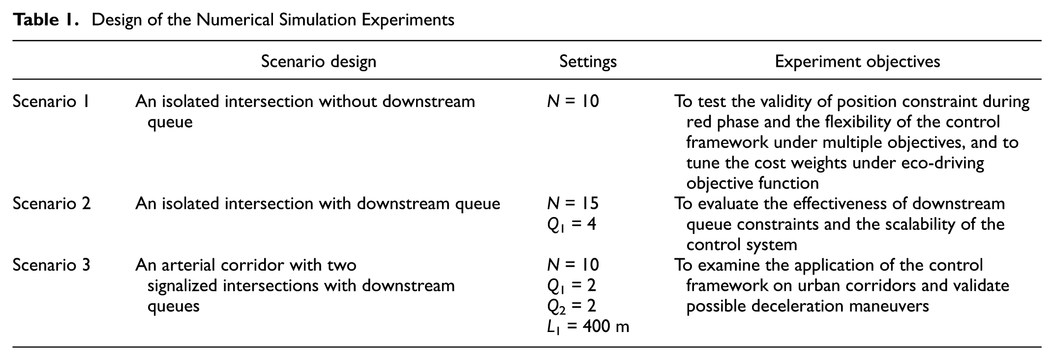
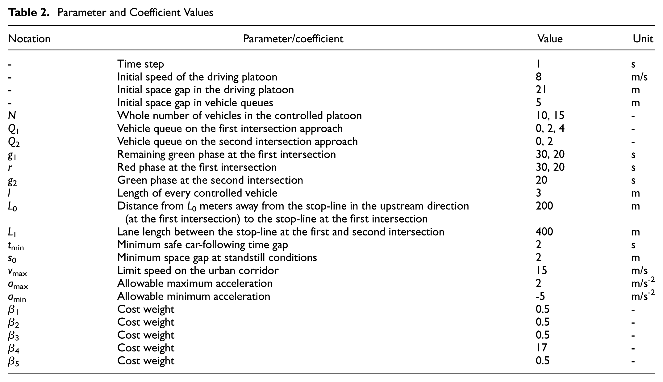
Three scenarios are designed to test the performance of the controlled CAV platoon for different experiment objectives. Table 1 describes the experiment design. The parameter values in the simulation are detailed in Table 2.

Table 1.

Design of the Numerical Simulation Experiments

	Scenario design	Settings	Experiment objectives
Scenario 1	An isolated intersection without downstream queue	N = 10	To test the validity of position constraint during red phase and the flexibility of the control framework under multiple objectives, and to tune the cost weights under eco-driving objective function
Scenario 2	An isolated intersection with downstream queue	N = 15 Q₁ = 4	To evaluate the effectiveness of downstream queue constraints and the scalability of the control system
Scenario 3	An arterial corridor with two signalized intersections with downstream queues	N = 10 Q₁ = 2 Q₂ = 2 L₁ = 400 m	To examine the application of the control framework on urban corridors and validate possible deceleration maneuvers

Table 2.

Parameter and Coefficient Values

Notation	Parameter/coefficient	Value	Unit
-	Time step	1	s
-	Initial speed of the driving platoon	8	m/s
-	Initial space gap in the driving platoon	21	m
-	Initial space gap in vehicle queues	5	m
N	Whole number of vehicles in the controlled platoon	10, 15	-
Q ₁	Vehicle queue on the first intersection approach	0, 2, 4	-
Q ₂	Vehicle queue on the second intersection approach	0, 2	-
g ₁	Remaining green phase at the first intersection	30, 20	s
r	Red phase at the first intersection	30, 20	s
g ₂	Green phase at the second intersection	20	s
l	Length of every controlled vehicle	3	m
L ₀	Distance from L₀ meters away from the stop-line in the upstream direction (at the first intersection) to the stop-line at the first intersection	200	m
L ₁	Lane length between the stop-line at the first and second intersection	400	m
t _min	Minimum safe car-following time gap	2	s
s ₀	Minimum space gap at standstill conditions	2	m
v _max	Limit speed on the urban corridor	15	m/s
a _max	Allowable maximum acceleration	2	m/s⁻²
a _min	Allowable minimum acceleration	−5	m/s⁻²
β ₁	Cost weight	0.5	-
β ₂	Cost weight	0.5	-
β ₃	Cost weight	0.5	-
β ₄	Cost weight	17	-
β ₅	Cost weight	0.5	-

Scenario 1 represents the situation where the controlled platoon splits into two at an isolated intersection without downstream queue on the approach in the prediction horizon (Q₁ = Q₂ = 0). The simplest Scenario 1 is simulated to verify if the optimal control framework works when the red phase is included as a position constraint. In Scenario 1, the first q vehicles of the driving platoon are expected to pass directly and the subsequent N−q vehicles cannot depart because of the red phase. The prediction horizon T is 60 s (T = g₁+r), including remaining green phase and red phase at the most upstream (first) intersection. To magnify the control effects of all cost terms and then obtain insights into tuning cost weights, the fuel consumption rates and speeds of all these N vehicles are optimized within the prediction horizon. The updated objective function is described in Equation 15. Performances in Scenario 1 could help understand how the control framework works under multiple objectives and prove the flexibility of the control approach, because of the changeable criteria in the objective function.

\min_{u, q} J = \min_{u, q} \int_{0}^{T} (β_{1} \sum_{i = 1}^{N} a_{i}^{2} (t) - β_{2} \sum_{i = 1}^{N} v_{i} (t) - β_{3} q + β_{4} \sum_{i = 1}^{N} f_{v} (v_{i} (t), a_{i} (t))) d t

(15)

Scenario 2 introduces a downstream vehicle queue at an isolated signalized intersection based on Scenario 1 (Q₁ = 4, Q₂ = 0), which provides insights into the effectiveness of the control approach regarding the downstream queue. Apart from the driving platoon, Q₁ vehicles are set to stop behind the stop-line waiting for the green phase at the start of the optimization. In Scenario 2, not only the split of the driving platoon but the merging of two platoons and the acceleration behavior of queuing vehicles at the start of green phase can be tested. In addition, an increase in the number of controlled vehicles (N = 15) could validate the scalability of the control system.

The forthcoming Scenario 3 is designed along a corridor of two signalized intersections, considering not only platoon splitting and merging again, but also downstream queues on two intersection approaches. Here the position constraints and initial information of position and speed are different from the previous scenarios. The remaining green phase g₁ is from t = 0 s to t = 20 s, the red phase r at the first intersection is between t = 21 s and t = 40 s, and the green phase at the downstream (second) intersection g₂ is set from t = 41 s to t = 60 s. Thus the prediction horizon T is 60 s, including not only the remaining green phase and red phase at the first intersection, but also the green phase at the second intersection. These controlled N (=10) vehicles include Q₁ (=2) and Q₂ (=2) vehicles waiting for the green phase behind the stop-line at the first and the second intersection separately, and N−Q₁₋Q₂ (=6) vehicles driving from L₀ meters away from the stop-line in the upstream direction at the first intersection. Given a short lane length (L₁ = 400 m) between two intersections, q passing vehicles at the first intersection may experience deceleration maneuvers between the stop-line at the first and second intersection. These q vehicles are expected to pass the first and second intersections as soon as possible but decelerate to keep safe gaps between two intersections. It should be noted that Q₂ vehicles on the second intersection approach are optimized only during the green phase at the second intersection g₂ to simplify computational complexity, which means these Q₂ vehicles remain stationary behind the stop-line during tε[0, g₁+r]. Scenario 3 could help validate the flexible characteristic of the control framework regarding the application on an arterial corridor of multiple signalized intersections with queues.

The three scenarios are appropriate to verify the platoon trajectory control approach. Owing to the characteristics of the control approach that every constraint and every criterion in the objective function could be exerted on any controlled vehicle over the prediction horizon, similar settings (e.g., the number of controlled vehicles, vehicle queues behind the stop-line at intersections, and the number of multiple intersections along a corridor) could be implemented in the same way. In addition, the communication ranges of V2I, I2V, and V2V are limited to about 200 meters in reality, thus the control approach starts from L₀ (200) meters away from the stop-line in the upstream direction at the first intersection. The distance between the upstream intersection and the downstream intersection L₁ is set to be 400 m to verify the possible deceleration maneuvers.

Platoon Performance

The three scenarios described above are simulated to evaluate control effects based on trajectory analysis, as depicted in Figures 2 to 4. The horizontal red lines in these figures show the red signal indication on the approach. It seems clear that all trajectories are able to satisfy the controller constraints, including the safe gap, allowable acceleration, and limited speed constraints. The remainder of this section analyzes the controlled platoon performances in different scenarios. Finally, three comparison baseline scenarios are implemented using the intelligent driver model under the same settings as the three scenarios. The simulation results should reveal the differences between CAV traffic control and intelligent driver model, and the potential of the proposed control approach in comparison with human drivers.

Figure 2.

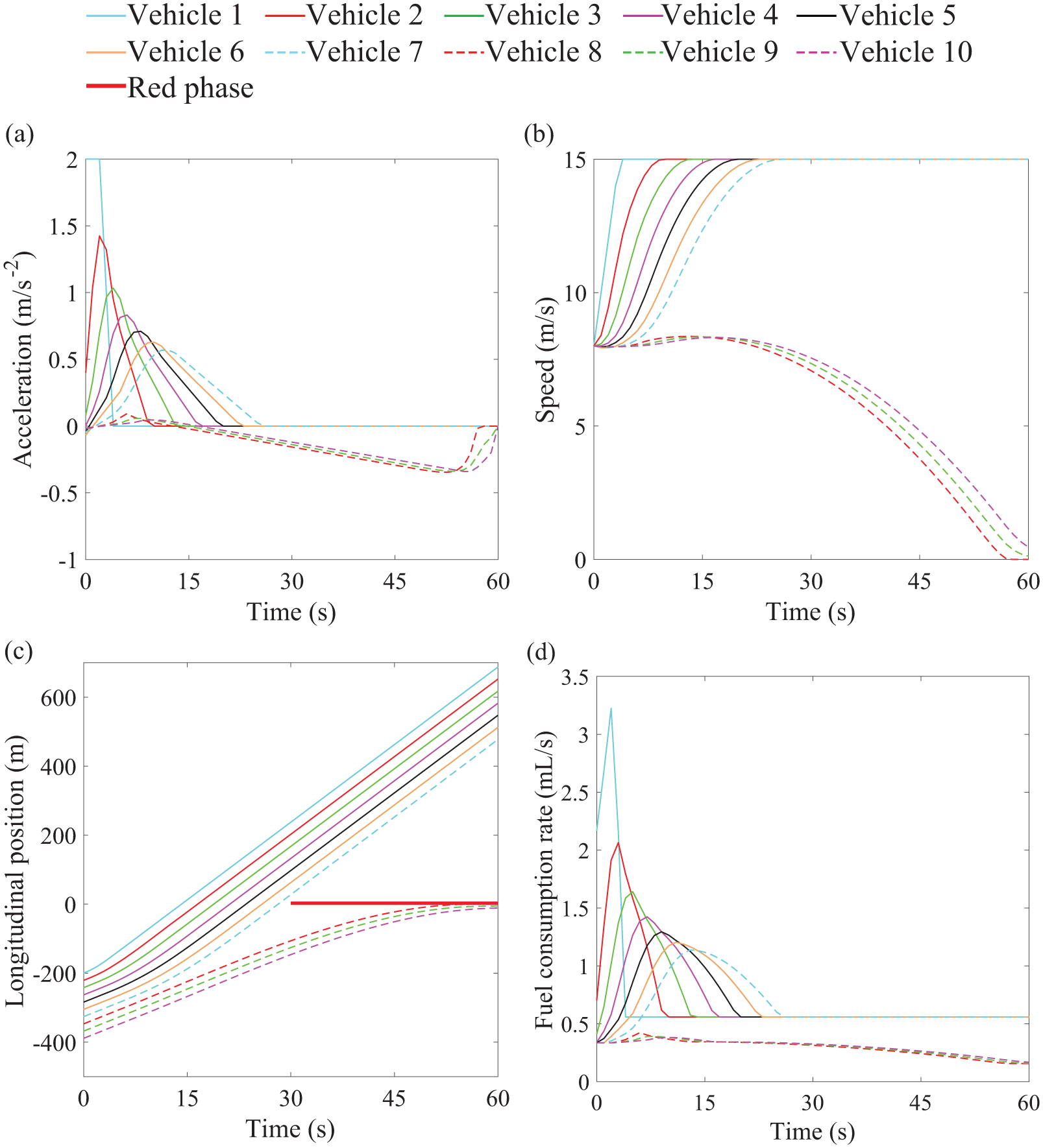
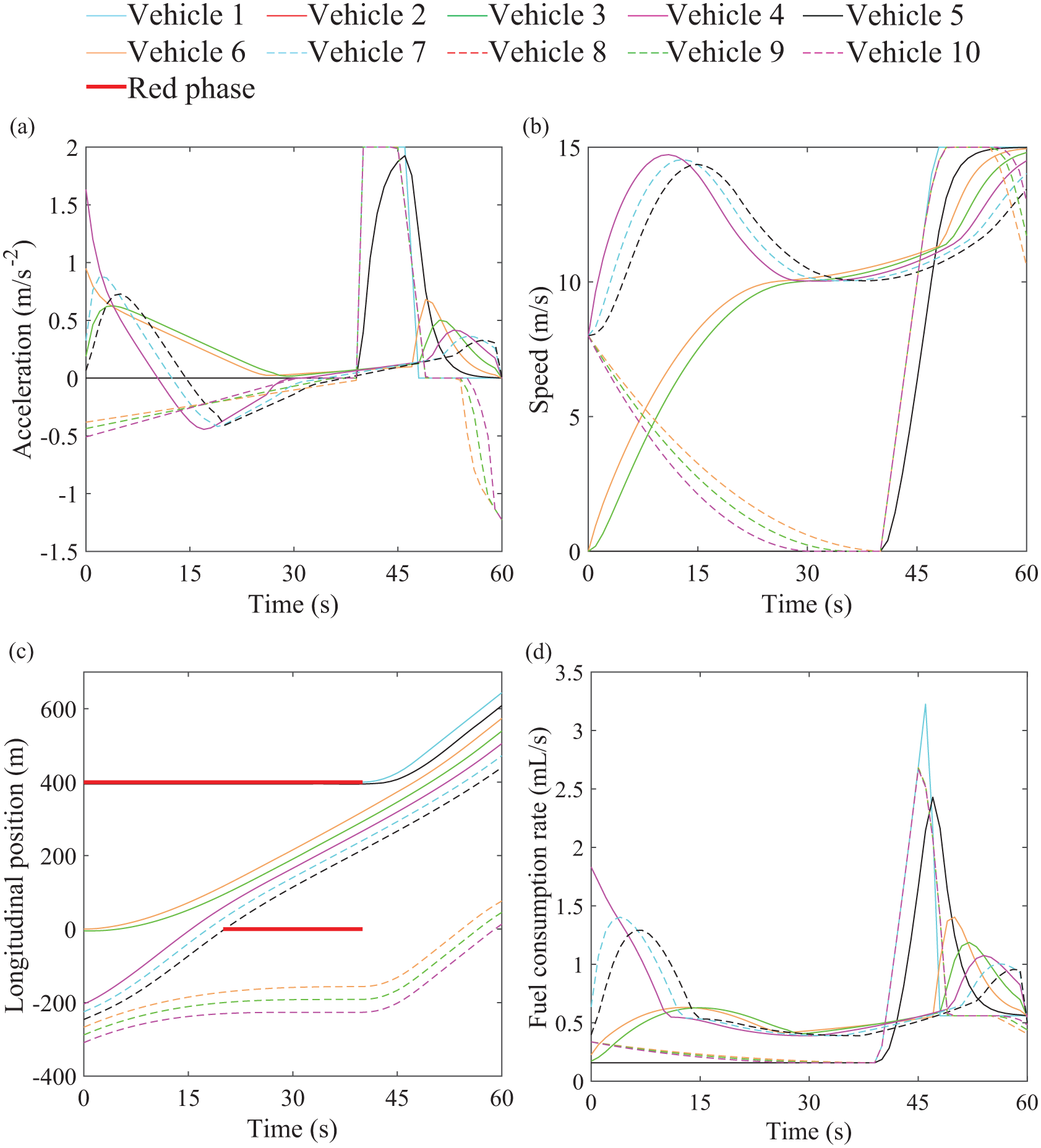
Optimized trajectories in Scenario 1: (a) acceleration; (b) speed; (c) longitudinal position; and (d) fuel consumption rate.

Figure 3.

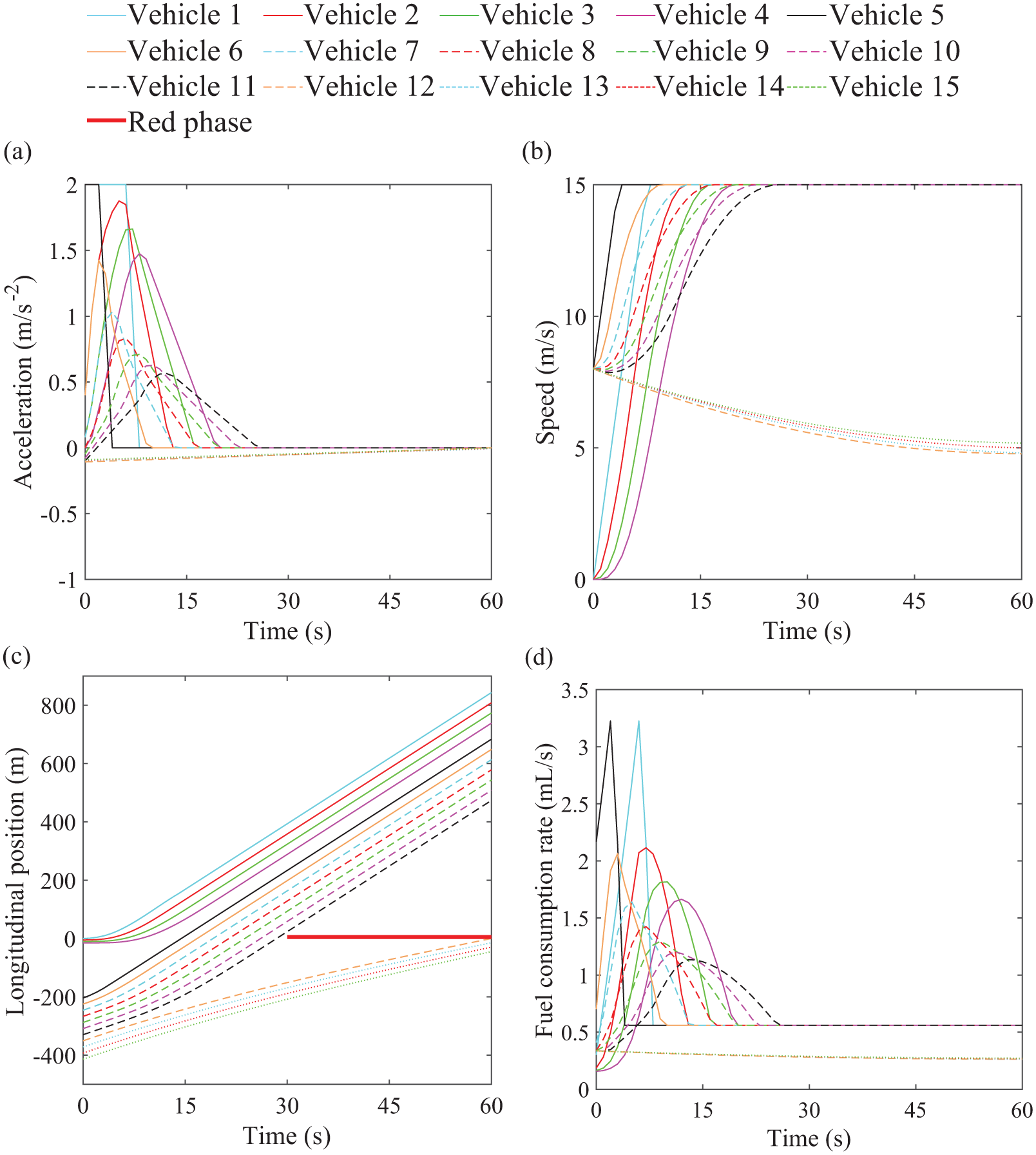
Optimal trajectories in Scenario 2: (a) acceleration; (b) speed; (c) longitudinal position; and (d) fuel consumption rate.

Figure 4.

Optimal trajectories in Scenario 3: (a) acceleration; (b) speed; (c) longitudinal position; and (d) fuel consumption rate.

Analysis of Scenario 1

In Scenario 1, the cost terms of minimizing the travel delay (maximizing vehicle speeds) and minimizing fuel consumption are implemented in all controlled vehicles within the prediction horizon, to magnify the effects of all criteria in the objective function. First, β₁ = 0.5 is regarded as a baseline. The choice of β₃ (= 0.5) does not influence the optimal solution because q is a constant in the objective function. The cost weight of speed, β₂, is supposed to keep the same order as the cost weight of acceleration β₁, thus β₂ = β₁ = 0.5. As to the fuel consumption cost weight β₄, it is found that bigger values of β₄ (>17) will overweight the fuel consumption cost term, causing lower speeds with respect to the first q vehicles when passing through the intersection. The objective function is to maximize the speeds of all vehicles, thus an overweighted fuel consumption cost weight β₄ has a negative influence on trajectory performances, especially speeds. To achieve the maximum speed with respect to the first q vehicles, the cost weight should not be overweight to be bigger than 17. Therefore, 17 is the maximum value of β₄ whereby the first q vehicles can achieve the maximum speed and all vehicles can achieve their optimal operations. As to Scenario 3, with two intersections, the same value is chosen as β₂ for the cost weight β₅ because of the same criteria.

Scenario 1 simulates the simplest experiment with only one intersection approach, and it seems clear that the control works well subject to all constraints and system dynamics. Vehicle 1 to 10 represents vehicle sequence number of the driving platoon on the lane, where the value of M₁ equals 9 and q is optimized to be 7. In Figure 2, only the first q (= 7) vehicles are leaving the intersection, while the subsequent N−q (= 3) vehicles cannot catch the green phase. It is shown that the first q vehicles accelerate quickly until the limit speed v_max and then keep a constant speed. Only Vehicle 1 reaches the maximum acceleration at the beginning, because it does not have to satisfy the safety constraint as the followers do. Vehicles that cannot pass the intersection decelerate and slowly approach the stop-line, because of an explicit optimization function of fuel consumption rate. Performances in Scenario 1 prove the flexibility of the control approach in that multiple criteria in the objective function could be applied, not limited to linear and quadratic objectives. In addition, criteria could be applied to arbitrary vehicles in the controlled platoon.

Analysis of Scenario 2

In Figure 3, platoon performances at an isolated intersection with downstream queue are depicted. The first Q₁(= 4) vehicles in the legend present the vehicle queue Q₁ on the signalized intersection approach. The maximum number of vehicles that could depart at the first intersection, q, is optimized to be 11. It is shown that the last N−q (= 4) vehicles cannot catch the green phase and stop behind the stop-line. Similar trajectories appear as for Scenario 1 in Figure 2 in relation to the split of the driving platoon. Using a position constraint to express the red phase, it is clear that the implementation of the downstream queue works in the optimal control approach.

Analysis of Scenario 3

In Scenario 3, the maximum number of vehicles passing in the remaining green time at the first intersection M equals 6. The value of q is optimized to be 5. It is clear that the driving platoon from L₀ meters away from the stop-line in the upstream direction at the first intersection splits into two parts and merges with the preceding platoon (Q₁ and Q₂) when the signal status changes (t = 20 s and t = 40 s). Acceleration and deceleration trajectories of all controlled vehicles are operated considerably smoothly because of the control objective of maximizing driving comfort.

The trajectories of the driving platoon in Figure 4 seem reasonable. The first q (= 5) vehicles (Vehicle 3 to 7) accelerate from the start, departing the first intersection directly. The leader in the driving platoon (Vehicle 5) begins with acceleration of 1.6 m/s², and the following two vehicles speed up with smaller accelerations. The first q (= 5) vehicles in the driving platoon are expected to accelerate to the maximum speed and then keep the limit speed v_max, but they cannot because of the short lane length (L₁ = 400 m) and constraint on safe gap. The last three vehicles in the driving platoon (Vehicle 8 to 10) are instructed to pass the stop-line at the first intersection by using a position constraint at the end of the second green phase (t = 60 s). Vehicles 8 to 10 decelerate first, approaching the stop-line slowly owing to the red phase (as a position constraint), and then accelerate at the beginning of the next green phase (t = 40 s) at the first intersection. After passing the stop-line at the first intersection, that is, satisfying the position constraint at the end of the second green phase, these last three vehicles (Vehicle 8 to 10) perform to decelerate because of the fuel consumption criteria in the objective function.

The trajectories of vehicle queues on the intersection approaches are explained as follows. The vehicle queue Q₁ (Vehicle 3 and 4) starts acceleration from stationary condition at the beginning of the green phase at the first intersection and moves to the second intersection with gradually increasing speeds but declining accelerations. The vehicle queue Q₂ (Vehicle 1 and 2) accelerates suddenly when the signal status turns green at the second intersection (t = 40 s), but vehicles in Q₁ at the first intersection accelerate at a smaller rate compared with Q₂ at the second intersection. This is because Q₁ vehicles are operated to maintain a safe gap with Q₂ vehicles with minimum acceleration fluctuations in the objective function. Q₁ vehicles therefore approach the vehicle queue Q₂ at the second intersection with a relatively slow increase in speed.

Instantaneous fuel consumption rates are calculated based on acceleration and speed. Speed trajectories are developed from the optimized accelerations, thus fluctuations in instantaneous fuel consumption rate are closely related to variations in acceleration, as shown in Figure 4d. The fuel consumption rates of vehicle queue Q₂ (Vehicle 1 and 2) maintain 0.16 ml/s in front of the stop-line at the second intersection when idling.

To show the behavioral differences and potential of the controlled platoon, three comparison baseline scenarios are designed with same settings as in Scenario 1, 2, and 3 based on the intelligent driver model. The simulation results are shown in Figure 5. The maximum number of vehicles that could pass the intersection is evaluated first when implementing the intelligent driver model on a corridor during the green phase. Later, a virtual stationary vehicle is inserted at the stop-line between the last passing vehicle and the first vehicle that has to stop at the red phase. After adding the virtual vehicle(s), the intelligent driver model is implemented again to simulate the trajectories under fixed-timing signal control. The virtual vehicle is removed after the green phase starts.

Figure 5.

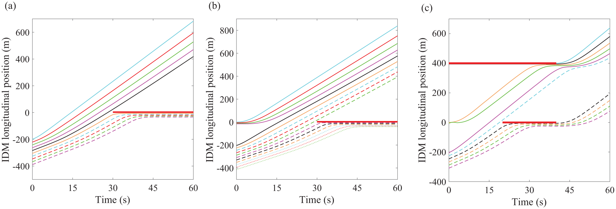
Longitudinal trajectories of intelligent driver model in (a) Scenario 1; (b) Scenario 2; and (c) Scenario 3.

Figure 5 shows the results of the simulation with the intelligent driver model. It is obvious that the optimal throughputs in this model are worse than their counterparts in the control approach. In Scenario 1, seven vehicles are able to leave while the control approach leads to two more vehicles passing the intersection, and the same finding holds for Scenario 2. In Scenario 3, one more vehicle leaves under the control approach compared with the intelligent driver model. In addition, the total fuel consumption of all controlled vehicles, by integrating the instantaneous fuel consumption rate in time, is also an advantage of the control approach. For instance, the fuel saving of the control approach in Scenario 3 is 18.4509 ml.

Conclusions and Future Work

This study proposed a flexible CAV acceleration control approach on urban roads that optimizes traffic operations with multiple criteria of throughput, driving comfort, travel delay, and fuel consumption, subject to safety and physical constraints. The control approach takes downstream vehicle queues into account and can be applied not only at an isolated signalized intersection but on urban arterials as well. The proposed control approach is applied to design the controller, the performance of which is verified by simulation with multiple intersections and downstream vehicle queues. In addition, changes in the criteria that constitute the objective function can be achieved straightforwardly in this framework, which also reveals the flexible characteristics of the control approach. Simulation results show that the proposed control system is able to achieve the control objectives and to satisfy the constraints. Further research is directed to the inclusion of multi-lane scenarios and real-time signal controls based on V2I information. Furthermore, research on relaxing the assumption of 100% penetration rate will be conducted in the future, including the consideration of system errors using robust or stochastic control, the queue estimation (of human drivers) using CAV information, and the control design in a mixed traffic flow of human drivers and CAVs.

Footnotes

Acknowledgements

The research presented in this paper is funded by the Chinese Scholarship Council (CSC).

Author Contributions

The authors confirm contribution to the paper as follows: study conception and design: ML, MW, SH; analysis and interpretation of results: ML, MW; draft manuscript preparation: ML, MW, SH. All authors reviewed the results and approved the final version of the manuscript.

The Standing Committee on Intelligent Transportation Systems (AHB15) peer-reviewed this paper (19-05632).

References

Guler

S. I.

Menendez

Meier

Using Connected Vehicle Technology to Improve the Efficiency of Intersections. Transportation Research Part C: Emerging Technologies, Vol. 46, 2014, pp. 121–131.

Yang

Rakha

Ala

M. V.

Eco-Cooperative Adaptive Cruise Control at Signalized Intersections Considering Queue Effects. IEEE Transactions on Intelligent Transportation Systems, Vol. 18, 2017, pp. 1575–1585.

Wang

Daamen

Hoogendoorn

S. P.

Van Arem

Connected Variable Speed Limits Control and Car-Following Control with Vehicle-Infrastructure Communication to Resolve Stop-and-Go Waves. Journal of Intelligent Transportation Systems, Vol. 20, 2016, pp. 559–572.

Wang

Daamen

Hoogendoorn

S. P.

van Arem

Rolling Horizon Control Framework for Driver Assistance Systems. Part I: Mathematical Formulation and Non-Cooperative Systems. Transportation Research Part C: Emerging Technologies, Vol. 40, 2014, pp. 271–289.

Wang

Daamen

Hoogendoorn

S. P.

van Arem

Rolling Horizon Control Framework for Driver Assistance Systems. Part II: Cooperative Sensing and Cooperative Control. Transportation Research Part C: Emerging Technologies, Vol. 40, 2014, pp. 290–311.

Han

Chen

Ahn

Variable Speed Limit Control at Fixed Freeway Bottlenecks using Connected Vehicles. Transportation Research Part B: Methodological, Vol. 98, 2017, pp. 113–134.

Fountoulakis

Bekiaris-Liberis

Roncoli

Papamichail

Papageorgiou

Highway Traffic State Estimation with Mixed Connected and Conventional Vehicles: Microscopic Simulation-based Testing. Transportation Research Part C: Emerging Technologies, Vol. 78, 2017, pp. 13–33.

J. Q.

Zou

Investigation of the Impacts of Signal Timing on Vehicle Emissions at an Isolated Intersection. Transportation Research Part D: Transport and Environment, Vol. 16, 2011, pp. 409–414.

Akcelik

Efficiency and Drag in the Power-Based Model of Fuel Consumption. Transportation Research Part B: Methodological, Vol. 23, 1989, pp. 376–385.

10.

Ahn

Rakha

Trani

Van Aerde

Estimating Vehicle Fuel Consumption and Emissions Based on Instantaneous Speed and Acceleration Levels. Journal of Transportation Engineering, Vol. 128, 2002, pp. 182–190.

11.

Rakha

Ahn

Trani

Development of VT-Micro Model for Estimating Hot Stabilized Light Duty Vehicle and Truck Emissions. Transportation Research Part D: Transport and Environment, Vol. 9, 2004, pp. 49–74.

12.

Kamal

M. A. S.

Mukai

Murata

Kawabe

Ecological Vehicle Control on Roads with Up–Down Slopes. IEEE Transactions on Intelligent Transportation Systems, Vol. 12, 2011, pp. 783–794.

13.

Shao

Sun

Wang

Bared

Huang

Integrated Optimal Eco-Driving on Rolling Terrain for Hybrid Electric Vehicle with Vehicle–Infrastructure Communication. Transportation Research Part C: Emerging Technologies, Vol. 68, 2016, pp. 228–244.

14.

Rakha

Kamalanathsharma

R. K.

Eco-Driving at Signalized Intersections using V2I Communication. Proc., 14th International IEEE Conference on Intelligent Transportation Systems (ITSC), Washington, D.C., 2011, pp. 341–346.

15.

Kamalanathsharma

R. K.

Rakha

H. A.

Multi-Stage Dynamic Programming Algorithm for Eco-Speed Control at Traffic Signalized Intersections. Proc., 16th International IEEE Conference on Intelligent Transportation Systems (ITSC), The Hague, Netherlands, 2013, pp. 2094–2099.

16.

Kamalanathsharma

R. K.

Rakha

H. A.

Yang

Networkwide Impacts of Vehicle Ecospeed Control in the Vicinity of Traffic Signalized Intersections. Transportation Research Record: Journal of the Transportation Research Board, 2015. 2503: 91–99.

17.

Lee

Park

Development and Evaluation of a Cooperative Vehicle Intersection Control Algorithm under the Connected Vehicles Environment. IEEE Transactions on Intelligent Transportation Systems, Vol. 13, 2012, pp. 81–90.

18.

Lee

Park

B. B.

Malakorn

J. J.

Sustainability Assessments of Cooperative Vehicle Intersection Control at an Urban Corridor. Transportation Research Part C: Emerging Technologies, Vol. 32, 2013, pp. 193–206.

19.

Zohdy

I. H.

Rakha

H. A.

Intersection Management via Vehicle Connectivity: The Intersection Cooperative Adaptive Cruise Control System Concept. Journal of Intelligent Transportation Systems, Vol. 20, 2016, pp. 17–32.

20.

Krajewski

Themann

Eckstein

Decoupled Cooperative Trajectory Optimization for Connected Highly Automated Vehicles at Urban Intersections. Intelligent Vehicles Symposium (IV), IEEE, Gothenburg, Sweden, 2016, pp. 741–746.

21.

Mandava

Boriboonsomsin

Barth

Arterial Velocity Planning Based on Traffic Signal Information under Light Traffic Conditions. Proc., 12th International IEEE Conference on Intelligent Transportation Systems (ITSC), St. Louis, MO, 2009, pp. 1–6.

22.

Asadi

Vahidi

Predictive Cruise Control: Utilizing Upcoming Traffic Signal Information for Improving Fuel Economy and Reducing Trip Time. IEEE Transactions on Control Systems Technology, Vol. 19, 2011, pp. 707–714.

23.

Xia

Boriboonsomsin

Barth

Dynamic Eco-Driving for Signalized Arterial Corridors and Its Indirect Network-Wide Energy/Emissions Benefits. Journal of Intelligent Transportation Systems, Vol. 17, 2013, pp. 31–41.

24.

Katsaros

Kernchen

Dianati

Rieck

Zinoviou

Application of Vehicular Communications for Improving the Efficiency of Traffic in Urban Areas. Wireless Communications and Mobile Computing, Vol. 11, 2011, pp. 1657–1667.

25.

Katsaros

Kernchen

Dianati

Rieck

Performance Study of a Green Light Optimized Speed Advisory (GLOSA) Application using an Integrated Cooperative ITS Simulation Platform. Wireless Communications and Mobile Computing Conference (IWCMC), Istanbul, Turkey, July 4–8, 2011.

26.

Stevanovic

Kergaye

Green Light Optimized Speed Advisory Systems: Impact of Signal Phasing Information Accuracy. Transportation Research Record: Journal of the Transportation Research Board, 2013. 2390: 53–59.

27.

Dridi

El-Moudni

Multi-Vehicles Green Light Optimal Speed Advisory Based on the Augmented Lagrangian Genetic Algorithm. In 2014 IEEE 17th International Conference on Intelligent Transportation Systems (ITSC), Qingdao, China, 2014, pp. 2434–2439.

28.

Stebbins

Hickman

Kim

H. L.

Characterising Green Light Optimal Speed Advisory Trajectories for Platoon-Based Optimisation. Transportation Research Part C: Emerging Technologies, Vol. 82, 2017, pp. 43–62.

29.

Seredynski

Dorronsoro

Khadraoui

Comparison of Green Light Optimal Speed Advisory Approaches. Proc., 16th International IEEE Conference on Intelligent Transportation Systems (ITSC), The Hague, Netherlands, 2013, pp. 2187–2192.

30.

Altan

O. D.

Barth

M. J.

Boriboonsomsin

Stark

J. A.

Glidepath: Eco-Friendly Automated Approach and Departure at Signalized Intersections. IEEE Transactions on Intelligent Vehicles, Vol. 2, 2017, pp. 266–277.

31.

Hao

Boriboonsomsin

Barth

M. J.

Eco-Approach and Departure (EAD) Application for Actuated Signals in Real-World Traffic. IEEE Transactions on Intelligent Transportation Systems, Vol. 99, 2018, pp. 1–11.

32.

Liu

H. X.

Liu

Optimal Vehicle Speed Trajectory on a Signalized Arterial with Consideration of Queue. Transportation Research Part C: Emerging Technologies, Vol. 61, 2015, pp. 106–120.

33.

Feng

Liu

H. X.

Spatiotemporal Intersection Control in a Connected and Automated Vehicle Environment. Transportation Research Part C: Emerging Technologies, Vol. 89, 2018, pp. 364–383.

34.

Feng

Liu

H. X.

Yang

Integrated Optimization of Traffic Signals and Vehicle Trajectories at Isolated Urban Intersections. Transportation Research Part B: Methodological, Vol. 112, 2018, pp. 89–112.

Optimal Platoon Trajectory Planning Approach at Arterials

Abstract

Control Formulation

Design Assumptions and Description of the Control Problem

Control Objectives

System Dynamics Model

Optimal Control Problem Formulation

Controller Constraints

Solution Approach

Simulation Results and Analysis

Experiment Design

Platoon Performance

Analysis of Scenario 1

Analysis of Scenario 2

Analysis of Scenario 3

Conclusions and Future Work

Footnotes

Acknowledgements

Author Contributions

References