Capacity,Capacity Drop,and Relation of Capacity to the Path Width in Bicycle Traffic

Abstract

Bicycle usage is encouraged in many cities because of its health and environmental benefits. As a result, bicycle traffic increases which leads to questions on the requirements of bicycle infrastructure. Design guidelines are available but the scientific substantiation is limited. This research contributes to understanding bicycle traffic flow by studying the aggregated movements of cyclists before and after the onset of congestion within the setting of a controlled bottleneck flow experiment. The paper quantitatively describes the relation between capacity and path width, provides a qualitative explanation of this relation by analyzing the cyclist configuration for different path widths, and studies the existence of a capacity drop in bicycle flow. Using slanted cumulative curves and regression analysis, the capacity of a bicycle path is found to increase linearly with increasing path width. A steady drop in flow rate is observed after the onset of congestion, indicating that the capacity drop phenomenon is observed in bicycle traffic. The results presented in this paper can help city planners to create bicycle infrastructure that can handle high cyclist demand.

The worldwide trend of urbanization leads to an increasing demand of people traveling from A to B within the city bounds. To handle this growing stream of travelers and prevent overloading of the road network, there is a need to transport people in a sustainable manner ( 1 ). Using the bicycle is a good option as long as the infrastructure allows a safe and quick journey. However, the current understanding of bicycle traffic is rather limited, leaving municipalities and practitioners with questions on how to create a cycling network that can handle a high cyclist demand.

Before looking at the network level, the traffic dynamics on a single bicycle path must be better understood. More specifically, the capacity of a bicycle path is of interest as well as how capacity relates to the path width. If the cyclist demand exceeds the capacity, congestion will occur which might impact the maximum flow along the bicycle path. This phenomenon, called the capacity drop, is observed in motorized traffic but has not been reported yet for bicycles. Insight into this phenomenon for cyclists will contribute to the overall understanding of bicycle flow and help practitioners to design cycling infrastructure that is sustainable in a future with increased bicycle demand.

This research contributes to understanding bicycle traffic by analyzing the aggregated movements of cyclists before and after the onset of congestion. The work is done within the setting of a controlled bottleneck experiment to minimize the influence of other traffic modes.

In the remainder of this paper, an overview of the literature is given first, followed by an explanation of the setup of the experiment. The resulting dataset is then described and the methodology to analyze the data is presented. Finally, the results are presented and discussed.

Background

Bicycle traffic has been the subject of research for more than three decades but the understanding of bicycle flow dynamics has progressed only little. In earlier years, Botma and Papendrecht ( 2 ) and Navin ( 3 ) have studied bicycle flow and have estimated the capacity of bicycle paths, which have motivated a range of similar studies ( 4 – 6 ). The reported capacity values show a large range between 2,600 and 8,100 bicycles per hour (cyc/hr). These differences, linked to the underlying cycling behavior, are not yet fully understood. Differences may occur because of the large variation in infrastructure such as the path width but this has not been tested yet. To better compare the reported capacity values, the relation between capacity and path width should be better comprehended.

To better grasp the dynamics of bicycle flow, Chen et al. ( 7 ) and Zhang et al. ( 8 ) have looked into finding similarities to the dynamics of motorized traffic and pedestrian flow. The comparisons show similar flow characteristics such as the occurrence of stop-and-go waves. Also, after scaling the speed and density with the mode-specific free-flow speed and length, a similar shape of the fundamental relation between density, speed, and flow has been retrieved. Jiang et al. ( 9 ) have looked specifically into bicycle flow and have found no evidence for a capacity drop. The capacity drop is a phenomenon that is frequently observed in car traffic flow after congestion occurs at a bottleneck. Because of the increased distance between drivers induced by acceleration, the discharge rate of the traffic jam can be lower than the free-flow capacity before the onset of congestion ( 10 ). The magnitude of the drop is determined by the intra-driver differences in preferred acceleration ( 11 ) and for vehicular traffic, capacity drops ranging from 3% to 30% are reported. The earlier mentioned study by Jiang et al. ( 9 ) is based on single-file movement of cyclists, which restricts the normal cycling behavior. Whether the capacity drop exists when cyclists are allowed to overtake is still an open question.

In pedestrian research, the relation between capacity and bottleneck width is described by Hoogendoorn and Daamen ( 12 ). They have found that pedestrians moving uni-directionally through a narrowing organize themselves in dynamic layers and move in a staggered fashion. This zipping behavior leads to a step-wise relation between capacity and bottleneck width; depending on the number of effective lanes that fit on the path, capacity increases in discrete steps. Similar behavior could be present in bicycle flow but this has not been studied so far.

In this work, we investigate the relation between capacity and path width. To this end, we carry out a cycling experiment with a realistic one-directional bicycle flow in which overtaking is explicitly allowed to occur. This allows for observing the free-flow capacity as well as the queue discharge rate. In this setting, the capacity drop phenomenon might be observed in the same way as in vehicular traffic. More details of the experiment are given in the following section.

Experiment

The experiment is held on a closed terrain to exclude the disturbance of other traffic participants such as cars or pedestrians. The cycling movements are recorded on a straight stretch so that cyclists can move at their free speed without being restricted by the road curvature. The experiment has been approved by the Ethics Committee of the Delft University of Technology. Further details of the track layout and camera placement are described later in this section but before elaborating on that, the paper continues with explaining the experimental design.

Design

The experiment consists of a group of cyclists that move along a uni-directional bicycle path. An obstacle is placed on the path that creates a bottleneck by narrowing the path and enables the occurrence of congestion (see Figure 1). The obstacle limits the flow since fewer cyclists fit on the path. However, the bottleneck is only activated when the cyclist demand exceeds the capacity, leading to congestion at the upstream side of the obstacle. To ensure the activation, participants should arrive at the bottleneck cycling at their desired speed with a sufficient rate.

Figure 1.

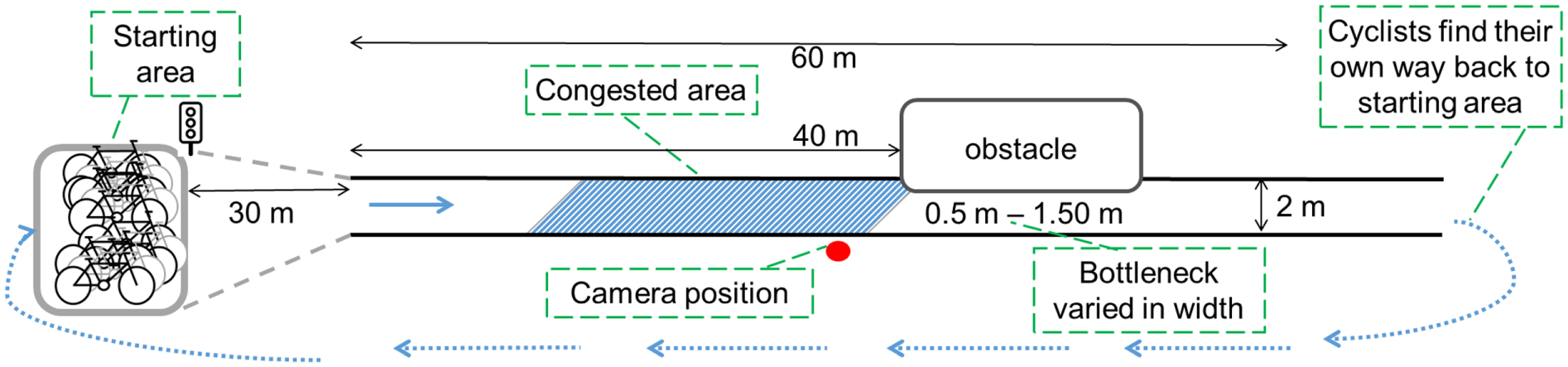
Sketch of the track design.

The capacity for different path widths can be determined before congestion sets in by varying the bottleneck width and ensuring a sufficient demand on the 2-m-wide path approaching the obstacle. If the capacity drop phenomenon occurs in bicycle traffic, the observed flow through the bottleneck will drop to the queue outflow rate after the onset of congestion.

Setup and Execution

The experiment was held in March 2018 on the Green Village terrain of Delft University of Technology in The Netherlands. The surface consists of 2 × 2 m concrete slabs over a total length of 60 m, creating a clear cycle path of width 2 m which is further indicated by orange cones (see Figure 2a). The participants, gathered in a starting area before the entrance of the track, start cycling after a start sign is given. The space between the starting area and the entrance of the cone-marked path is approximately 30 m, as illustrated in Figure 1. Multiple test runs confirmed that a length of 25 m is sufficient for individual cyclists to reach their desired speed from standstill. However, the start-up process of a group of 34 cyclists might take longer. Although we have not tested this hypothesis, we deem a total length of 70 m sufficient for the group to reach the bottleneck location at the desired speed. To ensure a high arrival rate at the bottleneck location, which is needed to find capacity, the cyclists start from a waiting area much wider than the 2-m path and they are vocally encouraged to start cycling simultaneously. This is to prevent the process of acceleration to the desired speed leading to stretching of the group configuration. Furthermore, the cyclists are instructed to cycle as they would normally do when leaving from a controlled intersection. After reaching the end of the 60-m stretch, the participants are asked to gather again at the starting point to prepare for the next run.

Figure 2.

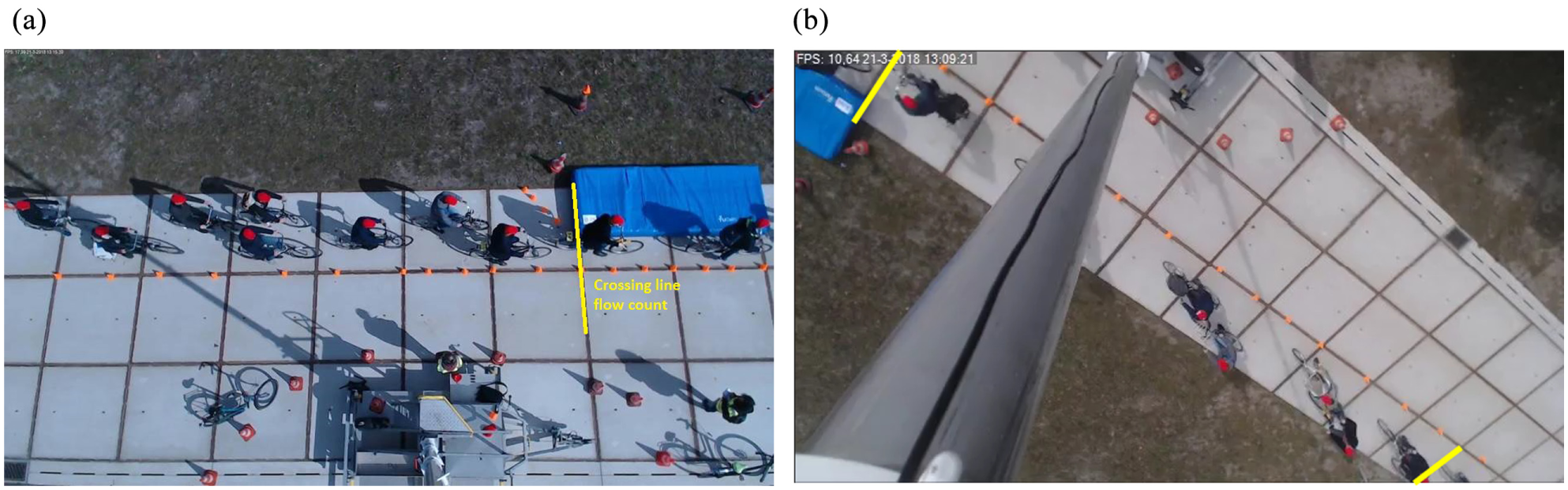
(a) View of camera 1 taken from a run with a 0.75-m-wide bottleneck and (b) camera 2 showing a situation with a 1.50-m-wide bottleneck. The crossing lines in yellow are used for the flow counts.

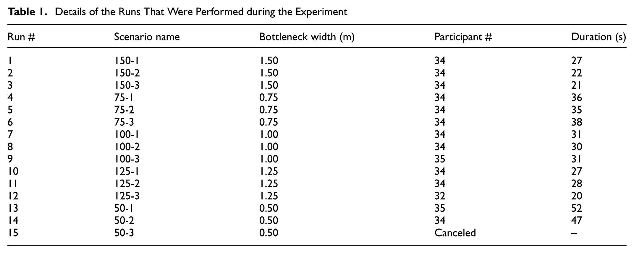
The obstacle, consisting of two inflatable air mattresses wrapped in a blue cover, is placed at approximately 2/3 of the straight stretch. The height of the obstacle is 33 cm which will block the pedaling over it but does not hinder steering which could be unsafe. Five scenarios are tested involving different bottleneck widths, varying between 0.50 and 1.50 m in steps of 25 cm. The order in which the scenarios are executed is randomized to reduce the behavioral adaptation. This results in the following order in which the scenarios are tested: 1.50, 0.75, 1.00, 1.25, and 0.50 m. Each scenario is repeated three times in a row to check for consistency.

Observations

In total, two cameras are placed on either side of an 11-m-high pole, which is positioned next to the track at the upstream side of the bottleneck. Camera 1 is the main camera and captures all bicycle movements from a near top-down angle on the stretch between 10 m upstream and 2 m downstream of the bottleneck entrance (Figure 2a). Camera 2 is placed as backup and records the cyclists over a stretch of 18 m with an angle towards the upstream side. The placement position at the other side of the pole creates a gap in the track recording because of occlusion by the pole (Figure 2b).

The recruitment of participants was done primarily via a master course at the university, resulting in a group of 34 people. A short questionnaire was handed out before starting the experiment to collect socio-demographic data on age, gender, nationality, bike type, and cycling experience. For privacy reasons, the survey data was anonymized and participants were asked to wear a red cap during the experiment to minimize face-recognition.

Dataset Description

A total of 34 people participated in the experiment and based on the survey result we know that the group consists mainly of students who use the bike on a daily basis. One participant stated that his/her cycling frequency is once per month; all others cycle on a daily basis. The percentages of male and female participants are 76% and 24% respectively and every participant joined with a bike that they are familiar with. Most of these bikes are classified as a regular bike which includes a wide range of bikes with different braking systems (hand-brake or back-pedal brake) and one or multiple gears. Three exceptions are mentioned explicitly because they might lead to different behavior: 1) a foldable bike, which has a different physical shape, 2) a fixed gear bike, which has a different acceleration pattern, and 3) a racing bike, which has a different pose and desired speed. The details on age and nationality of the participants are presented in Figure 3. These descriptive data might be useful when comparing our results to future studies.

Figure 3.

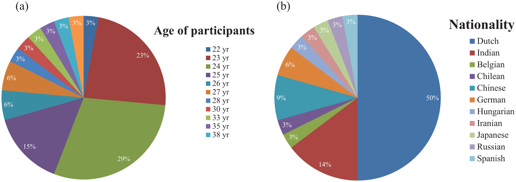
Socio-demographic data of the 34 participants.

A total of 14 runs are recorded and in most runs 34 participants joined. Some runs have 32 or 35 people because participants dropped out or one of the organizers joined in as well. An overview of the runs is presented in Table 1. The third run of the scenario with a bottleneck width of 0.50 m (run 50-3) was canceled for safety reasons. The path was so narrow that some cyclists were touching the obstacle with their pedal or moving the cones, creating a potentially unsafe situation for the following cyclists.

Table 1.

Details of the Runs That Were Performed during the Experiment

Run #	Scenario name	Bottleneck width (m)	Participant #	Duration (s)
1	150-1	1.50	34	27
2	150-2	1.50	34	22
3	150-3	1.50	34	21
4	75-1	0.75	34	36
5	75-2	0.75	34	35
6	75-3	0.75	34	38
7	100-1	1.00	34	31
8	100-2	1.00	34	30
9	100-3	1.00	35	31
10	125-1	1.25	34	27
11	125-2	1.25	34	28
12	125-3	1.25	32	20
13	50-1	0.50	35	52
14	50-2	0.50	34	47
15	50-3	0.50	Canceled	–

The next section describes the process and choices that are made to extract the data from the video recording.

Data Extraction

All cycling movements are captured by the main camera 1 and the backup camera 2 (see Figure 2). The recording frequency of camera 1 fluctuates around 15 frames per second because of frame skipping, whereas backup camera 2 operates with a lower frequency of around 10 frames per second. The frame rate fluctuation results in irregular position shifts of cyclists between frames, making a frame-by-frame analysis of bicycle displacements difficult. To minimize this error, only the first frame of every second is used for further analysis.

The camera recordings were programmed to save every 15 min while maintaining a continuous data stream. However, this process did not function properly, resulting in gaps of two to three minutes between recordings in which data was lost. As a result, the scenarios 50-1 and 50-2 were not fully captured by main camera 1, and backup camera 2 was used for the data extraction instead.

The data extraction of the flow rate is done manually by counting the number of cyclists that have passed the bottleneck entrance in each second as indicated by the yellow lines in Figure 2. If a cyclist is situated across a boundary, the center of a bicycle, in between the two wheels, is used to determine its position. As pointed out by Steffen and Seyfried ( 13 ), there are downsides to using this definition. The continuous nature of the cycling movement is lost because of the discretization of space and time. The space discretization leads to a volatility in the dataset since the cyclists who are moving across a boundary are either in or out based on the bike’s center point, while in truth they are spread across the crossing line. Furthermore, the resulting data depends on the chosen aggregation time. This error can be reduced by averaging over time but at the cost of the data resolution. In our case, we base the further analysis on the moving mean of 3 s and leave a more detailed analysis for future research.

Data Analysis Plan

The objectives of the paper are to quantitatively describe the relation between capacity and path width, and to check the existence of a capacity drop in bicycle flow. To meet the objectives, both free-flow capacity and queue discharge rate for the different bottleneck widths need to be estimated. First, we will present the method we use to find the individual capacities; then we describe the process to determine the path width dependency of capacity.

Estimating Capacity

A first indication for capacity is obtained by visualizing the time it takes for all cyclists to pass the bottleneck. This is done by constructing a cumulative flow curve for each run. This curve indicates how many cyclists have passed a particular location as function to time. Hence, the cumulative flow number $N$ is constructed by adding up all the flow counts of the previous time steps. The slope represents the number of cyclists that pass the bottleneck per time step, which equals the flow $q=\frac{\mathrm{dN}}{\mathrm{dt}}$ . The steeper the curve the higher the flow, so capacity coincides with the steepest curve. The cumulative flow curves for the different runs are presented in Figure 4. The moment that the first cyclist enters the narrow section is chosen as the starting time (t = 0). The first 10 s are chaotic and the lines are difficult to distinguish. This part can be ignored since the main message of the figure relates to the range between 10 and 50 s. It illustrates that for narrower bottlenecks (gray and purple colors) the time needed to let all cyclists pass increases compared with the wide bottleneck widths (black and red colors). In the widest bottleneck (150 cm) it takes at least 21 s, whereas the passing time in the narrowest bottleneck (50 cm) is at most 52 s.

Figure 4.

Cumulative curves of the runs with bottleneck widths between 0.50 and 1.50 m. The legend refers to the scenario names as given in Table 1.

To obtain the capacity value, a so-called slanted cumulative flow curve is used, indicated by $\tilde{N}$ . This means that a constant reference flow ( $q_0$ ) is subtracted from the cumulative flow count ( $N$ ) resulting in the expression:

$$\tilde{N}=N-\int q_0\mathrm{dt}$$

(1)

By changing the reference flow, one can slant the curves in such a way that the $\tilde{N}$ is constant. This is done manually by choosing different values for $q_0$ . The advantage of this is that the capacity value can be determined accurately and there is no influence of aggregation time. To remove noise, we use a 3-s moving average.

Capacity values are determined for each run separately. We find a value for both the free-flow capacity as well as the queue discharge rate. Hence, we find two values for which there is a constant value of the slanted cumulative flow curve. If a capacity drop exists, two steady plateaus should be identified in the slanted curve. The highest value coincides with the free capacity and should occur before congestion occurs, whereas the lower value is the outflow capacity which would occur after the onset of congestion. The difference between the two capacity values is the capacity drop.

Figure 5 shows graphically the working of the methodology for the run 75-1, resulting in a capacity value of 1.45 cyc/s and queue outflow rate of 0.83 cyc/s. Other determined capacity values are presented in Section 6.

Figure 5.

Example of slanted cumulative curves to determine (a) capacity and (b) queue outflow rate (run 75-1). The blue line is based on the 1-s data and the red line is the 3-s moving average. The black lines are added to illustrate the horizontal plateau.

Quantifying the Path Width–Capacity Relation

When the capacity and outflow rates are determined for all bottleneck widths, the dependency to path width can be quantified using linear regression analysis. This will result in the capacity equation:

$$C=C_0+\beta d.$$

(2)

where $C$ is the capacity in cyc/s of a $d$ -meter wide path. Furthermore, $\beta$ is the regression coefficient which coincides with the slope of the regression line when the equation is plotted. The physical interpretation of this coefficient is that an additional meter of path width coincides with an increase in capacity by $\beta$ cyc/s. The regression constant $C_0$ is the y-intercept of the capacity equation. Hypothetically, this gives the capacity of a path of 0-m width, which is an unrealistic situation. Therefore, $C_0$ does not have a physical interpretation.

Qualitative Description of the Width–Capacity Relation

The dependency of capacity to path width is expected to stem from the underlying cycling behavior. This can be assessed by providing a qualitative description of the cyclists’ configuration while passing the bottleneck.

To describe the position of cyclists, the path is divided into lanes and sub-lanes using the description of Botma and Papendrecht ( 2 ) to determine the cyclist headway. A cyclist occupies a lane which is approximately as wide as its steer. These individual lanes are not fixed to the path but have a dynamic position on the path based on the cyclist wheels. The path itself is divided into fixed sub-lanes of width 15.6 cm. These sub-lanes are used to describe the lateral position of the cyclists. If the wheels of following cyclists have a displacement of 15.6 cm or more, the cyclists are assigned to a different sub-lane. Since the individual lanes at the path edges cannot be shifted, the total number of sub-lanes on a path is equal to the path width divided by 15.6 minus two. A lane is assigned “effective” when it is used by the cyclists.

Results

In this section we present the results. We first report on the quantitative analyses of the capacity before discussing qualitatively the relation between path width and the observed flow configurations.

Capacity and Capacity Drop

For all runs, both a capacity value as well as a queue outflow rate are obtained using slanted cumulative curves. All estimated flow rates are combined into one graph, (see Figure 6). The line is a visualization of the regression fit and the measurements are indicated by points. It shows a positive trend of flow rates with increasing bottleneck width. The smallest capacity value of 0.90 cyc/s is obtained in the 0.50-m scenario, whereas the largest value of 2.4 cyc/s coincides with a run in the 1.50-m scenario. A similar trend is found for the outflow rate with the smallest value of 0.56 cyc/s and largest value of 1.99 cyc/s in respectively a 0.50-m and 1.50-m run.

Figure 6.

Estimated capacity values for each of the 14 runs. The black dots are the bottleneck capacities observed before congestion, whereas the red dots represent the queue outflow capacities that are observed after the onset of congestion. The two lines visualize the regression fits.

Fitting the relationship as mentioned in the earlier section results in Equation 3 for capacity $C_{\mathrm{cap}}$ and Equation 4 for the outflow rate $C_{\mathrm{out}}$ :

$$C_{\mathrm{cap}}=0.475+0.0111d$$

(3)

$$C_{\mathrm{out}}=0.042+0.0118d$$

(4)

The models have an R²-value of 0.896 for capacity and 0.949 for the outflow rate, which is a strong result. It means that the obtained equations can explain 89.6% and 94.9% respectively of the observed variance in estimated capacity and outflow rate.

The slope of the equations presented in Figure 6 quantifies the dependency of capacity to path width, which is what we set out to find. For an additional meter of path width in the range of 0.50 to 1.50 m, the capacity increases by 1.11 cyc/s and the queue outflow rate increases by 1.18 cyc/s. These slopes are remarkably similar and the difference is only 0.07 cyc/s, indicating that a constant drop in flow rate occurs after activation of the bottleneck. In the range of 0.50 to 1.50-m path width, the flow rate drops 0.45 cyc/s when the cycling conditions change from free flow to congested. These results provide evidence that the capacity drop phenomenon exists in bicycle traffic.

Cyclist Configuration and Its Connection to Capacity

If cyclists would behave like vehicles, the capacity would be dependent on their following distance and the number of lanes. For our bottleneck widths there are either one or two lanes since the standard lane width is between 0.75 and 1.00 m. This lane number is insufficient to explain the variation in capacity. The positive dependency of capacity to path width can be explained by qualitatively analyzing the cyclist configuration while passing the bottleneck, using sub-lanes and effective sub-lanes as introduced previously. This leads to the observations described in writing below, followed by an interpretation. A visualization of the different configurations is presented in Figure 7, illustrating examples of observed patterns:

• 2.00 m: Four effective sub-lanes are observed on the main path while approaching the bottleneck location. A maximum of two sub-lanes are occupied simultaneously, leading to a staggered formation in the lateral direction. Cyclists are not completely positioned side-by-side, but show a slight displacement in the longitudinal direction as well.

• 1.50 m: While passing the widest bottleneck, sufficient space is available to continue cycling side-by-side but the number of effective lanes reduces to about three, of which two can be occupied simultaneously. People on the right side occupy the same lane, while the ones on the left side can still vary their position in the lateral direction, occupying different sub-lanes.

• 1.25 m: Enough space remains available to cycle side-by-side but the choice in lateral position is limited. The cyclists on the left and right path are now using the same lane as their predecessor. Most people place themselves such that the saddles are not located side-by-side but the front and rear wheel can be completely overlapping when looking at a cross section.

• 1.00 m: The width is reduced such that cycling side-by-side is impossible and only one effective lane is occupied at the same time. In lateral direction, the placement is such that the rear and front wheel can be side-by-side, meaning that two effective lanes are used simultaneously. This enables cyclists to maintain a small distance to each other in longitudinal direction.

• 0.75 m: Only single-file movement is observed with only a small variation in lateral placement. Whether this displacement exceeds 15.6 cm and therefore uses one or two effective lanes cannot be judged based on the video images at this stage. It can be observed that the distance between cyclists increases compared with the 1.25-m path.

• 0.50 m: Again, only single-file movement is observed but now cyclists have an identical placement on the path, using the same effective lane. The longitudinal placement of cyclists increases even further compared with the previous bottleneck size.

Figure 7.

Sketch of cyclist configuration while moving from left to right along a path of different widths.

When visualizing the qualitative description of cyclist configuration for different bottleneck width, the sequence in Figure 7 shows resemblance to a merging process. The lateral distance between effective lanes gradually decreases until the path width does not allow cyclists to use multiple sub-lanes simultaneously, and the longitudinal distance between cyclists increases. Since merging is a gradual process, it can explain the linear expression of the relation between path width and capacity.

Discussion

The mentioned capacity values and queue discharge rates for the different bottleneck widths are obtained by conducting a bottleneck experiment with 34 cyclists. The group composition and socio-demographic characteristics of its participants, such as age or cycling experience, as well as the experimental setting, that is, the artificial bicycle path and bottleneck situation, may influence the capacity values. The results reported in this paper are therefore preliminary and should be validated in future research. This has not been done at this stage since the existing empirical data for bicycle flow is limited and no similar experiment has been conducted so far. In the future, it would be interesting to compare the findings with observations in real-world situations and to check the sensitivity to different types of bike paths and different group characteristics such as age or cycling experience.

The obtained linear expression of the capacity equation is explained in this paper by the resemblance to a merging process based solely on configuration of the cyclist while passing the bottleneck. Besides positioning, the average speed is also expected to influence the capacity. Although the speed is not quantified, the behavior observed in the video images provides indications that the average speed upstream of the bottleneck decreases with decreasing path width, that is, cyclists “anticipate” the approaching bottleneck and therefore reduce their speeds. This is reflected by an increase in observed swaying movements to prevent falling over and, as speed reduces further, people placing a foot on the ground for extra stability, resulting in stepping rather than cycling behavior. The bicycle itself remains in motion but the individual’s speed reduces close to zero when a foot is placed temporarily on the ground.

The cyclists anticipate their turn to pass the bottleneck entrance and accelerate before actually passing it. Therefore, the speed through the bottleneck is already higher than in the queue, and the flow observed at the bottleneck entrance is the queue discharge rate. The change from capacity to queue discharge rate is best visualized in the curves of the runs with 0.75-m bottleneck width in Figure 4. The flow is highest in the first 10 to 15 s (steep slope) and reduces to a steady flow (steady slope) afterwards.

A learning effect for the various bottleneck widths can be considered by looking into the duration of the consecutive runs (see Figure 8). Remarkably, the second run is typically shorter than the first run of each experiment, which might indicate a learning effect as cyclists become more familiar with the track. This trend however is less clear when comparing the third to the second run. Furthermore, it is not resembled in the obtained capacity values.

Figure 8.

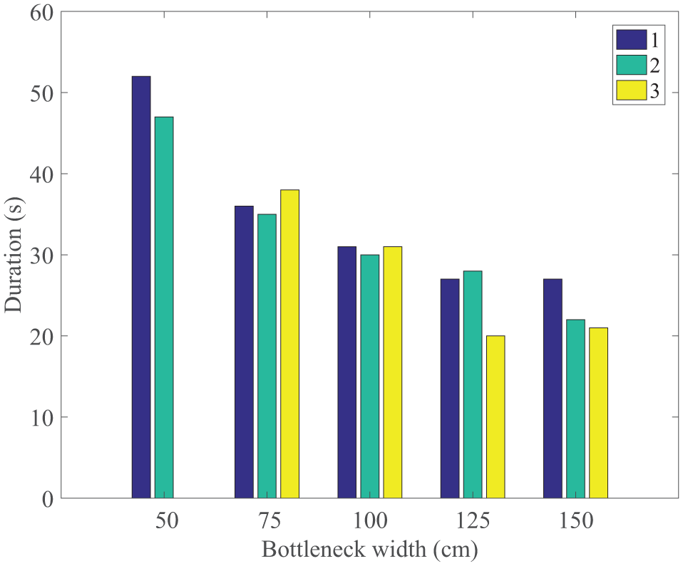
Total duration of the three consecutive runs within each bottleneck scenario.

The highest values for free-flow capacity however are observed in the 3rd, 1st, 2nd, 2nd, and 1st run of the different scenarios, while the highest outflow rates are observed four times in the 2nd run and once in the 3rd. This indicates that the learning effect is not consistently present.

Another explanation of the different run duration is the arrival pattern of the cyclists at the bottleneck location. Because of stretching of the group caused by speed differences or delays in the start-up process, the first cyclists arrived a few seconds before the rest of the group and thereby lengthened the total duration time. The effect of this stretched arrival pattern is illustrated by a flatter slope in the first 5 s of the cumulative curve in Figure 4.

The estimated relation between path width and capacity value can be used to find maximum flow values outside the range of 0.50–1.50 m. However, the bottleneck width of 0.50 m was difficult for the cyclists to pass and the third iteration of this scenario was canceled for this reason. A path width smaller than 0.50 m would be even more challenging and unrealistic in daily practice. Therefore, a 0.50-m path width is considered to be the minimum and as a consequence, the regression model should not be used to find capacity values for paths smaller than 0.50 m. This restriction does not apply to extrapolation for larger path widths when assuming that the usage of the path does not change. However, future research is advised to confirm that extrapolation is indeed allowed.

The non-zero y-intercept of the capacity equation indicates that observed capacity values on a certain path width, cannot be standardized to a capacity per meter by simply dividing it by the total path width. Instead, the result obtained in this study of 1.11 cyc/s per meter width can be used. By doing so, the wide range of capacity values reported in literature might be narrowed down, leading to a clearer advice for road planners.

Conclusion

A cycling bottleneck experiment was set up to study bicycle path capacity. The experiment involved a group of cyclists moving along a 2-m wide path which included an obstacle to create a bottleneck by narrowing the path. The size of the bottleneck was varied between scenarios ranging between 0.50 and 1.50-m width and each scenario was repeated three times. The flow rate before activation of the bottleneck (free-flow capacity) and the flow rate after the onset of congestion (queue discharge rate) were analyzed.

An important finding of this paper is that the capacity was found to be linearly dependent on the cycle path width. In fact, the capacity increases by 1.11 cyc/s for every additional meter path width in the range of 0.50–1.50 m. The queue outflow rate was also found to be linearly dependent on path width with an increase of 1.18 cyc/s/m. Both values can be used as reference value to compare capacities of cycling paths of various width. The queue discharge rate was found to be consistently lower than the free-flow capacity and the drop magnitude was 0.45 cyc/s for cycle path widths between 0.50 and 1.50 m. This confirms the existence of the capacity drop phenomenon in bicycle traffic.

The linear relationships for both the free-flow capacity and the queue discharge rate have yielded a non-zero constant. Therefore, the capacity values found for a certain path width cannot be standardized to a capacity per meter by simply dividing it by the total path width. This complicates the comparison of capacity values reported in literature, which typically focus on a single bottleneck width each. The result obtained in this study, which provides both the slope and the axis intercept, can be used to correct and compare capacities across different path widths. By doing so, the wide range of capacity values reported in literature might be narrowed down.

A qualitative analysis of the cyclist configuration has shown that the bicycle path capacity does not work with lanes as in car traffic, but sub-lanes can be formed. Hence, the capacity does not increase in large steps for one or two lanes only but smaller increases in cycle path width already lead to an increase in number of sub-lanes and the capacity therefore gradually increases.

Next steps in the research involve the retrieval of individual trajectories to enable the analysis of the density-flow relation based on individual localized densities. Furthermore, the obtained insights into bicycle flow dynamics will be used in the development and calibration of a macroscopic bicycle flow model. The development of such a model will enable the estimation of city-wide cyclist demand and, in the long term, help mitigate bicycle congestion.