Sage Journals: Discover world-class research

Abstract

Free-flow movement of vehicles in microsimulation software is usually defined by a set of equations with no explicit link to the instantaneous dynamics of the vehicles. In some cases, the car and the driver are modeled in a deterministic way, producing a driving behavior, which does not resemble real measurements of car dynamics or driving style. Depending on the research topic, the interest in microsimulation is to capture traffic dynamics phenomena, such as shockwave propagation or hysterisis. Existing car-following models are designed to simulate more the traffic evolution, rather than the vehicle motion, and consequently, minimal computational complexity is a strong requirement. However, traffic-related phenomena, such as the capacity drop are influenced by the free-flow acceleration regime. Furthermore, the acceleration pattern of a vehicle plays an essential role in the estimation of the energy required during its motion, and therefore in the fuel consumption and the CO₂ emissions. The present work proposes a lightweight microsimulation free-flow acceleration model (MFC) that is able to capture the vehicle acceleration dynamics accurately and consistently, it provides a link between the model and the driver and can be easily implemented and tested without raising the computational complexity. The proposed model is calibrated, validated, and compared with known car-following models on road data on a fixed route inside the Joint Research Centre of the European Commission. Finally, the MFC is assessed based on 0–100 km/h acceleration specifications of vehicles available in the market. The results prove the robustness and flexibility of the model.

Transportation systems comprise many complex elements (vehicle, infrastructure, driver, control systems, etc.) that might interact with each other at some point in time/space and they are often studied as a whole. The interactions within such systems introduce high stochasticity which, in some cases, makes the production of quantifiable results difficult or even impossible. As the studies go into greater depth of detail, the uncertainty increases. However, in some studies, the immersion in greater detail is not only essential but mandatory for the provision of reliable and robust conclusions. An example of such a case is the simulation of longitudinal vehicle free-flow movement, which is the topic of this paper. The observation of the traffic flow in a sophisticated transportation network, at a micro level, with various scenarios and different model parametrizations relies on the initial specifications, which profoundly affect the way the vehicles move and thus the final results of the study.

Car-following models explicitly reproduce the complex dynamics governing the actions of the driver-vehicle system, while the driver is following another vehicle. New car-following models are regularly proposed, and several studies provide reviews on the topic ( 1 – 3 ). A recent interesting review proposed by Zheng et al. ( 4 ) evaluates various typical car-following models such as the Gazis et al. ( 5 ) stimulus-response model, the Gipps model ( 6 ), the Newell model ( 7 ), the Optimal Velocity model ( 8 ), and the Cellular Automata model ( 9 ). One of the key conclusions is that there are noticeable differences between them and that those models with complex structures are more computationally expensive, while those with simpler structures do not offer good simulation performances. Furthermore, models with more parameters face over-fitting problems in validation, although they mimic real traffic accurately during the calibration process.

Traditionally, the deceleration pattern of the vehicle is considered as primarily responsible for the instability of the traffic flow. However, a free-flow acceleration regime is known to affect capacity drop ( 10 ) and possibly other traffic-related phenomena. Even though available traffic models are not able to capture such aspects without significant fine-tuning of their parameters, research on the reliability of the free-flow acceleration regime has been very limited ( 11 ).

Also, the acceleration pattern of a vehicle plays a vital role in the estimation of the energy required by a vehicle during its motion and, therefore, of the fuel consumption and the CO₂ emissions ( 12 – 14 ). During acceleration, vehicles tend to generate far more emissions than during cruising, idling, and deceleration ( 15 ). Furthermore, while traffic simulation models are used to perform environmental or energy-related impact assessment studies of various types of technology and traffic management solutions, little or no discussion is usually made on the robustness of such estimations (see for example [ 16 – 18 ]). In the literature, detailed and well-calibrated emissions estimation models are directly integrated with traffic models under the false assumption that the car-following models, which are used to simulate the power required by the vehicle to move in the integrated framework, were able to accurately reproduce the actual vehicle dynamics (see for example [ 19 – 21 ]).

The driver model can be an essential component in microsimulation. Unlike car-following models, driver models have the role of explicitly representing activities such as steering, gear-changing, or break- and accelerator-pedal control. All these actions have a powerful impact on the fuel consumption and emissions and, without considering—at least to the extent possible—these aspects, the entire effort of integrating the different models loses part of its meaning ( 22 ). In the literature the approaches that attempt to incorporate traffic, driver, and vehicle models are very few ( 23 – 26 ). A notable one, was carried out in the framework of the ICT-Emission project funded by the European Union ( 23 , 27 ). Another interesting approach is the Rakha and Lucic Vehicle Dynamics Model ( 24 ) proposed by Rakha et al. which is used to predict maximum light-duty vehicle accelerations for use within a microscopic traffic simulation environment. It uses readily available input parameters to estimate acceleration rates of small and large vehicles. However, one of the main drawbacks of this approach is the absence of the gear-shifting behavior and the assumption that the driver has the same acceleration behavior across the whole acceleration profile. The work proposed by Fadhloun et al. ( 25 ) extends and improves the Rakha and Lucic model by incorporating the driver behavior in the mathematical expression of the dynamics-based acceleration model. This model allows the simulation of different driver variations and it is validated on field data and its main differences with the proposed paper lie in the absence of a gear-shifting functionality and the fact that results refer only to vehicles with an automatic gearbox. Finally, another interesting work is a vehicle powertrain model proposed by Rakha et al. ( 26 ).

This work proposes the microsimulation a free-flow acceleration model (MFC) that is based on two calibratable parameters, gear-shifting style and driver style, as well as the vehicle specifications, which are used to compute the maximum acceleration that the vehicle can have at a given speed. The basis of the MFC is the vehicle acceleration curve, which represents the maximum acceleration that the car can achieve for a given speed which, in this work, is often noted as acceleration potential. On the top of the vehicle-specific curve, MFC is parametrized by the gear-shifting style and the driving style. Both elements are important mainly for the assessment and accurate estimation of the energy demand and efficiency of a transport system, comprised by a fleet of vehicles that can be diverse both in relation to size (small, medium, and large light-duty vehicles) and characteristics (hatchbacks, station wagons, pick-ups), but also propulsion and driving technology (hybrids, electric, automated vehicles etc.). MFC is simple to implement, it has low computational cost and, by comparison with both the Gipps ( 6 ) and the Intelligent Driver Model (IDM) ( 28 ), it proves its robustness for various vehicles, drivers, and driving styles. The rest of the paper describes the proposed model, the experimental set-up, and the experimental results The final section discusses the conclusions and future work.

MFC Free-Flow Model Description

The proposed methodology proposes the implementation of a lightweight microsimulation free-flow acceleration model (MFC) and proposes its implementation within the well-known Gipps car-following model by substituting the free-flow part. MFC can be calibrated based on two parameters to simulate different drivers. The acceleration of the vehicle at a given speed derives from the vehicle’s acceleration-speed curve and the profile of the vehicle’s driver. More specifically, the acceleration-speed curve defines the acceleration-speed space for the specific vehicle, as this is mathematically described by the interaction of the tractive forces and the resistances that apply at a given speed. In the present work, this is also called the acceleration potential of the vehicle. The driver’s profile is described by two parameters, the driver’s gear-shifting strategy and the driving style. The gear-shifting strategy correlates the shifting points when the driver changes gear with the power curve of the vehicle and thus the operating speed of the vehicle’s powertrain. The driving style defines the amount of the acceleration potential that a driver wants to use. The components mentioned above are sufficient to describe the vehicle and the human parts as well as their interaction during a vehicle’s acceleration. The MFC has been implemented and tested successfully both as a standalone free-flow model and inside a Gipps framework, with substitution of the corresponding free-flow part, in the Python-based custom simulator and in the SDK Application Programming Interface (API) of Aimsun.

The Acceleration-Speed Curve of the Vehicle

The acceleration-speed curve of the vehicle corresponds to the computed maximum acceleration achievable by the vehicle across the vehicle’s entire speed range (acceleration potential). The acceleration potential is thus a function of the current vehicle’s speed and the gear applied. To estimate the acceleration potential of a car, a simple vehicle longitudinal dynamics model and the full load curve of the vehicle’s powertrain are used as described below.

a_{c p} (v) = \frac{F_{m a x w h} (v, g e a r_{i}) - F_{r e s i s t a n c e s} (v)}{m_{c .}}

(1)

where

$a_{cp}$ is the acceleration potential,

$F_{maxwh}$ is the maximum tractive force that can be supplied to the vehicle’s wheels by the engine,

$v$ is the instantaneous vehicle velocity,

$gea r_{i}$ is the gear used,

$F_{resistances}$ is the sum of the forces resisting the vehicle motion in steady speed conditions, and

$m_{c}$ is the corrected inertia of the vehicle which accounts for the vehicle mass and the inertia of its rotating components.

In this study $m_{c} = 1.03 m$ where $m$ is the vehicle’s mass.

The $F_{maxwh}$ is calculated using the full load curve $T_{maxpt} (Spee d_{pt})$ of the vehicle’s powertrain and an efficiency factor ( $η_{dt}$ ) to account for the losses in the vehicle’s drivetrain system (gearbox, final drive). The full load curve expresses the maximum torque provided by the vehicle’s powertrain system as a function of powertrain speed ( $spee d_{pt}$ ).

F_{maxwh} (v, gea r_{i}) = T_{maxwheels} (v, gea r_{i}) / r_{dyn}

(2)

At this point, it should be added that an additional control is introduced in the model so that the maximum traction force delivered at the powered wheels cannot exceed the expected traction achievable by the vehicle’s tires in certain conditions. The latter is calculated based on the equation:

F_{maxlim} = g^{*} m^{*} {k_{frac}}^{*} μ

(3)

So, at any point in time $F_{maxwh} (v) \leq F_{maxlim}$ . In Equation 3, $g$ is the acceleration of gravity, $m$ is the vehicle mass, $k_{frac}$ is the fraction of the weight imposed on the powered wheels (typically 0.55, 0.45 and 1 for front-wheel driven, rear-wheel driven, and all-wheel driven vehicles, respectively), $μ$ is the friction coefficient which for normal conditions is considered as 1, for wet conditions 0.75 and snowy conditions 0.25

T_{maxwheels} (v) = T_{maxpt} (spee d_{pt}) \cdot n_{tot} / η_{dt}

(4)

where

$T$ stands for torque,

$spee d_{pt}$ is the output rotational speed of the powertrain,

$n_{tot}$ is the total transmission ratio of the drivetrain (gear ratio x final drive ratio),

$η_{dt}$ is an average efficiency factor considered for the losses in the drivetrain (in this study considered 0.92 for manual transmission vehicles and 0.9 for automatic transmission vehicles), and

$r_{dyn}$ is the dynamic rolling radius of the wheels.

The powertrain speed is calculated as

spee d_{pt} = v / (2 \cdot pi \cdot r_{dyn} \cdot n_{tot})

(5)

Several vehicle Original Equipment Manufacturers (OEMs) publish information on the full load curve of their vehicles’ powertrains which can be retrieved for various vehicles. In cases where the full load curve is not available a second option is used. The model contains a normalized generic full load curve. To de-normalize and obtain a realistic estimate of the full load curve for a specific engine, the maximum torque and power for the particular vehicle are used.

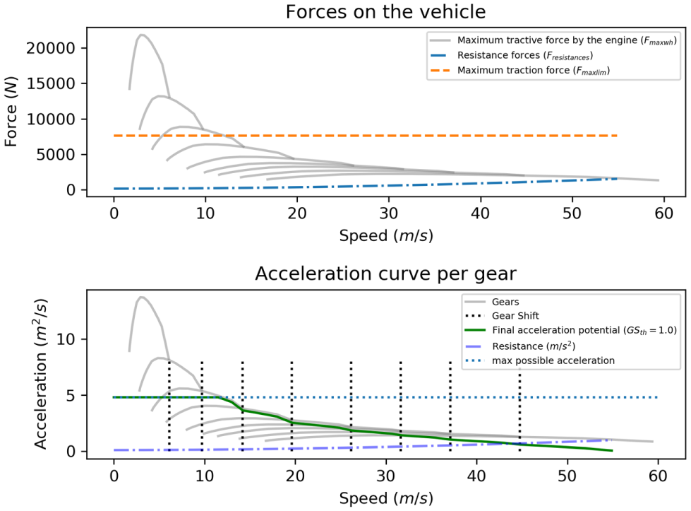
At this point, it should be noted that each gear results in different $F_{maxwh}$ curve. To obtain the overall $F_{maxwh}$ curve across the vehicle speed operation range, for the intervals where the curves of two gears overlap, the maximum force value is considered (see Figure 1).

Figure 1.

(top) Illustration of the various forces that apply on the vehicle across its speed range; and (bottom) Illustration of the resulting acceleration per gear, the gear-shifting points, and the final acceleration potential of the vehicle.

To calculate the maximum achievable acceleration, the resistance forces being applied at steady speed conditions on the vehicle are calculated based on the following equation and then subtracted from $F_{maxwh}$ .

F_{resistances} = (F_{0} \cdot \sin (φ) + F_{1} \cdot v + F_{2} \cdot v^{2} + m \cdot a + m \cdot g \cdot \cos (φ)

(6)

Variables $m$ and $g$ are the mass and acceleration of gravity respectively, while $φ$ is the road gradient. Factors $F_{0}$ , $F_{1}$ , $F_{2}$ are commonly used to characterize the road loads of vehicles; they express the constant part of a vehicle’s resistances (tire rolling resistances), the part that is proportional to velocity (partly tire rolling resistance, partly drivetrain losses), and the part that is proportional to the square of the vehicle’s velocity (aerodynamic component). A dedicated module for the calculation of the vehicle’s road loads was developed by Tsiakmakis et al. ( 29 ) and was adopted for the needs of this study. Figure 1 illustrates the forces that apply on the vehicle over the entire vehicle speed range. The MFC derives the acceleration potential based on the net result of the forces acting on it.

Gear-Shifting Strategy

Gear shifting is a complicated functionality that is not usually modeled explicitly in existing driver models applied in traffic simulation. Because of the stochasticity in the simulation of such an approach, the common logic in many models is to aggregate this error in a final error term over the final acceleration. The MFC proposes a gear-shifting strategy that correlates the shifting points with the power curve of the vehicle and thus the operating speed of the vehicle’s powertrain. More specifically, the force for each gear is described by the function $F_{maxwh, g_{i}} (v)$ , where $g_{i}$ is the gear and $v$ the speed in m/s. The the derivative of this funtion is computed as follows:

Ta n_{g_{i}} (v) = \frac{ϑ F_{maxwh, g_{i}}}{ϑ v}, \forall g_{i}

(7)

The value ranges of the $Ta n_{g_{i}}$ functions are normalized using unity-based normalization:

G S_{g_{i}} (v) = 1 - \frac{Ta n_{g_{i}} (v) - min (Ta n_{g_{i}} (v))}{(max (Ta n_{g_{i}} (v)) - min (Ta n_{g_{i}} (v)))}, \forall g_{i}

(8)

The range of possible values is $G S_{g_{i}} \in [0, 1]$ . A threshold value, here called $G S_{th},$ defines the gear-shifting point per gear. $G S_{th}$ can take any value between 0 (timid driver) and 1 (aggressive driver).

From the MFC implementation point of view, the driver upshifts on any speed $v_{k}$ when the $G S_{g_{i}} (v_{k}) \geq G S_{th} and G S_{g_{i}} (v_{k - 1}) < G S_{th}$ , $v_{k - 1}$ is the speed in the previous time instance. Correspondingly, the downshifting occurs when $G S_{g_{i}} (v_{k}) < (G S_{th} + c) and G S_{g_{i}} (v_{k - 1}) \geq (G S_{th} + c)$ , where $c$ is a relaxing constant parameter for downshifting (here set to 0.1), to prevent continuous gear shifting when a vehicle moves at a speeds around gear shifting points.

By choosing different $G S_{th}$ we manage to define different gear-shifting strategies. It is interesting to note that although there is a unique threshold for gear shifting, the shifting point at each gear and in each vehicle varies, as it depends on the gear curvature. The single threshold value keeps the number of a model’s parameters low and thus its complexity.

Furthermore, the vehicle’s acceleration potential for a given speed depends on the gear that is in the gearbox at that given speed. During the acceleration, shifting to a higher gear, the available power by the vehicle reduces. Therefore, early gear-shifting can lead to mild acceleration, while late gear-shifting leads to sharper acceleration. Figure 4 provides an illustrative representation.

Additionally, the implementation of the power loss of the vehicle during gear shifting for a fixed delay equal to $G S_{del}$ , is simulated in two ways depending on whether the vehicle has an automatic or manual transmission. In the first case, the power of the vehicle drops to $G S_{g_{i}} (v) / 2$ for time duration equal to $G S_{del}$ , while in the second case the power of the vehicle drops to zero for the same time. Empirically, for the moment, the $G S_{del}$ has been set to 0.5 seconds but this is something that needs to be calibrated in our future work.

Although the effect of gear shifting on the overall trajectory profile of a single vehicle might seem small, the authors believe that it can play an important role in instantaneous fuel consumption estimation for a vehicle or a vehicle fleet and furthermore on the traffic flow, especially on fleets with many vehicles having manual gear boxes. Two main parameters that affect both fuel consumption and traffic dynamics are the instantaneous speed and acceleration. Figure 2 illustrates two indicative acceleration-over-speed diagrams highlighting the measured and the simulated data using MFC after calibration with the method described in the section below on results.

Figure 2.

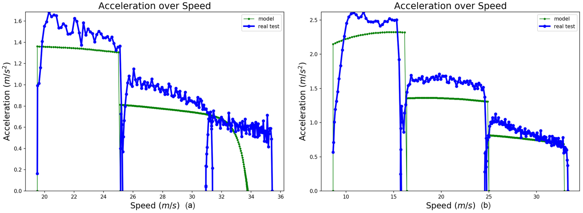
Acceleration over speed diagrams for indicative acceleration experiments and the corresponding fitted MFC model with gear shifting.

Driving Style

Supposing a driver wants to accelerate from a starting speed to a desired one, at each speed the acceleration value in the MFC depends on the capabilities of the vehicle, that is, how fast the vehicle can accelerate, bounded by the style of the driver—in other words, whether she drives aggressively or mildly—and on the difference between the current speed and the desired one. Consequently, in the present work, driving style is described by: a) the driver’s will to exploit the entire vehicle’s acceleration potential; and b) a function that dictates how the driver utilizes the selected potential, while approaching the desired speed.

Parameter $DS \in (0, 1]$ of the MFC is related to the willingness of the driver to exploit the vehicle’s full potential, as aggressive drivers tend to push the vehicle’s engine to the limits, while timid drivers do not. Consequently, $DS$ represents the ratio between the driver’s real acceleration over the vehicle’s theoretical capability and therefore $DS$ should take values closer to zero when we want to simulate a timid driver and closer to one for a more aggressive one.

The driver’s acceleration behavior as approaching the desired speed is simulated by a function $a_{w}$ , and it is defined as follows:

a_{w} (v_{i}) = {\begin{matrix} DS \cdot (1 - {(\frac{v_{i}}{V_{D}})}^{a}), when 0.5 < \frac{v_{i}}{V_{D}} \leq 1 \\ DS \cdot (1 - b \cdot {(1 - \frac{v_{i}}{V_{D}})}^{a}), when 0 \leq \frac{v_{i}}{V_{D}} \leq 0.5 \\ c^{*} (1 - (\frac{v_{i}}{V_{D}})), when \frac{v_{i}}{V_{D}} > 1 \end{matrix}

(9)

where $a$ and $b$ are constant values of the $a_{w} (v_{i})$ function and parameter $c$ (here set to 10) is a simplistic dumping coefficient to dictate the vehicle deceleration when a new desired speed, lower than the current one, is imposed on free flow. Parameters $a, b$ have been experimentally fit over acceleration data and optimal values have been set to 60 and 0.8 respectively.

The above formula is derived from a set of acceleration experiments performed at the JRC laboratories of the European Commission similar to the ones illustrated in Figure 3(top). More specifically, the tests involved 104 targeted acceleration tests in the Vehicle Emissions Laboratories (VELA) of the JRC with three passenger vehicles having different power characteristics, driven by five drivers instructed to accelerate normally. The measurements referred to 10 Hz. The starting and desired speeds were selected to correspond to a representative part of the speed range of the vehicle. 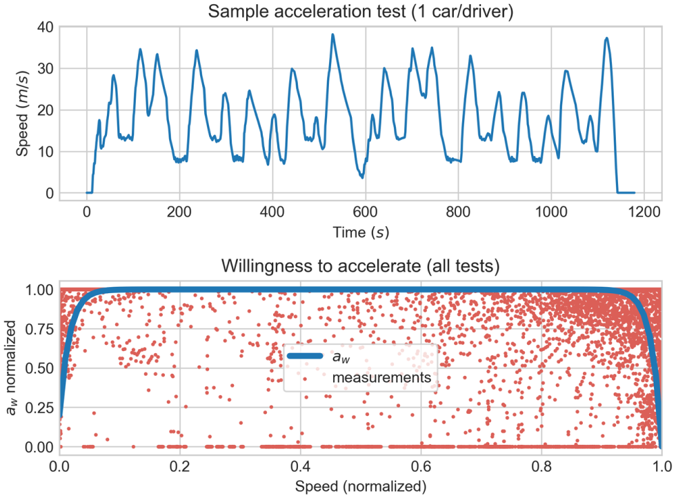Knowing a priori the road loads used in the chassis dynamometer and the vehicle characteristics, the acceleration potential of the vehicle was subtracted from the driver’s accelerations in the tests and the resulted measurements were further normalized according to the $DS$ of each acceleration test. The aim was to reveal the $a_{w}$ function.

Figure 3.

(top) A sample accelerations test cycle in the JRC VELA labs; and (bottom) scatter plot of the measured willingness of the driver to accelerate, as it is defined in this work, and the corresponding function $a_{w} (v_{i})$ to approximate it.

The result is shown in Figure 3(bottom). It is evident that in the biggest part of each acceleration test all drivers reached their individual $DS$ , but in the beginning of their acceleration exercise, and before reaching their desired speed, they performed lower acceleration values. In the same picture the $a_{w}$ seems to cover adequately this behavior.

Driver’s Acceleration-Speed Profile

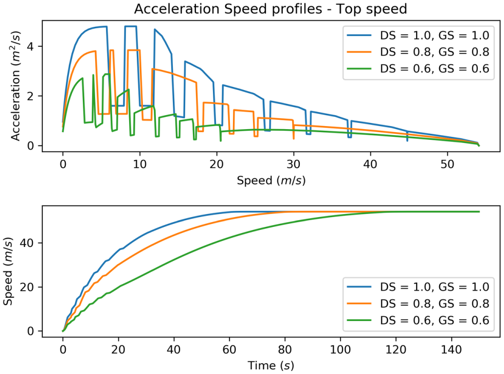
The sections above defined both MFC parameters, the driver’s will, $DS$ , and the gear-shifting strategy, based on the threshold $G S_{th}$ . Figure 4 depicts the profiles of three indicative drivers for the same vehicle. The first driver, $(DS, G S_{th}) = (1, 1)$ , is the most aggressive, as she exploits all of the vehicle’s acceleration potential, the second driver, $(DS, G S_{th}) = (0.8, 0.8)$ , is more timid and the third, $(DS, G S_{th}) = (0.6, 0.6)$ , is the most conservative. The third driver, changes gears too early and she reaches the last gear sooner, at around 22 m/s, thus losing the power to accelerate sharply. In the speed profiles shown in Figure 4(bottom), the different levels of aggressiveness are translated into time delays and it is interesting to observe the gear shifts.

Figure 4.

(top) Acceleration-speed profiles for three different drivers with different driving styles; and (bottom) the simulated speed profiles for the same drivers.

The calibration and validation in the experimental results section was performed with speed over distance profiles. The desired speed during such tests is a variable over distance, like the speed limit. In such tests, MFC should also be able to reduce speed when the updated speed limit is lower than the previous one. The third condition in Equation 11 ensures the model’s stable behavior. An example of the model’s response in such cases is given in Figure 5, where a fictional distance-based speed cycle is illustrated. The figure on the top shows the cycle and the simulation by the MFC, while the figure on the bottom shows the speed over time profile of the model for the same cycle.

Figure 5.

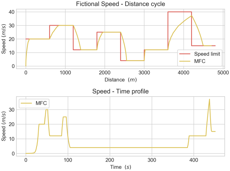
(top) Artificial speed-distance cycle with the response of the MFC; and (bottom) the speed-time profile of the MFC.

Implementation of the MFC in Microsimulation

The proposed work is focused on the design and development of a robust and lightweight free-flow model that can be used in microsimulation software. Consequently, as a first implementation version of the MFC, the authors substituted the free-flow part of the Gipps model with the MFC implementation described above. The hybrid version of the Gipps works easily without an increase in the complexity, apart from the introduction of the two MFC parameters $G S_{th}$ and $DS$ . In practice, the acceleration potential for the vehicle fleet can be computed offline once, and the MFC parameters can define a distribution of driver profiles without additional complexity. For the needs of the proposed paper, the MFC was implemented inside the Gipps framework in both python (toy networks) and C++ code (SDK API of Aimsun), without creating apparent/prohibitive delays (e.g., over real-time), even when used in complex scenarios with additional tasks such as the real-time estimation of the instantaneous fuel consumption for each vehicle in the network.

Experimental Set-Up

For the model development and validation, a series of tests took place to collect measured GroundTruth data. The experimental campaign was run in the fully-fenced Ispra site of the JRC, to avoid the interactions with other vehicles on the road, under free-flow conditions. A vehicle was equipped with a commercial multi-constellation Global Navigation Satellite System (GNSS) receiver able to collect GNSS data with a 10 Hz measurement rate. The receiver was configured to collect signals from both GPS and Galileo, the European GNSS. The average horizontal accuracy reported by the receiver was less than 50 cm. A GNSS active antenna was mounted on the roof of the car to ensure maximum satellite visibility and avoid signal attenuations from the body of the vehicle. Figure 6(left) depicts the set-up of the antenna on the vehicle. During the experiments conducted, the vehicle was moving on the predefined route shown in Figure 6(right), which is about 1.15 km long. The results presented in this work refer to 28 laps inside JRC on free-flow and position measurements every 0.1 seconds. The engine specifications for the vehicle are an engine capacity of 2000cc and 101kW power.

Figure 6.

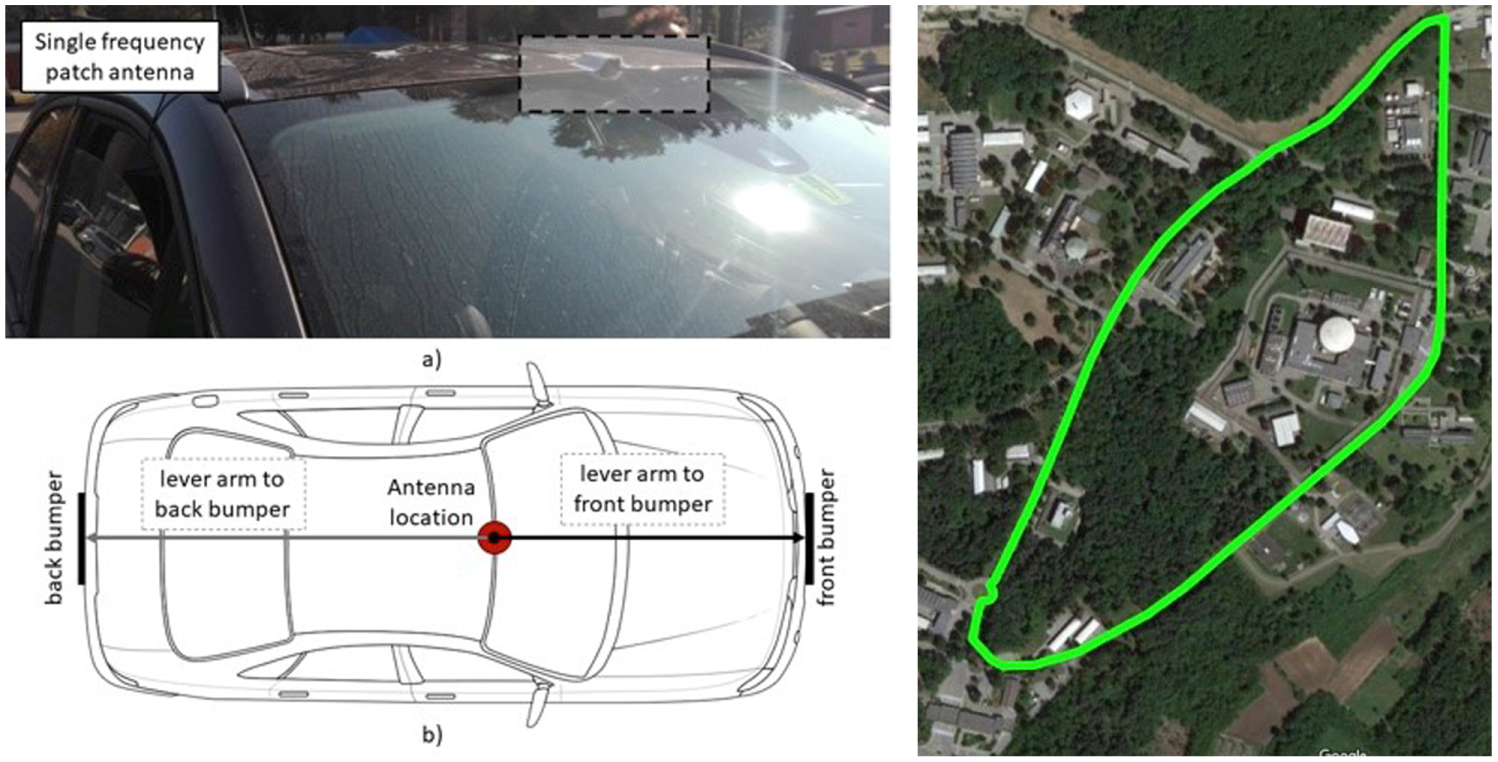
(left) Experimental set-up with the location of the GNSS antenna; and (right) the path used for the experiments inside the JRC Ispra site.

The measured trajectory profile (distance-over-time) per lap of the test vehicle was transformed to a distance-over-speed profile. The latter was used as a GroundTruth basis for the comparison of the three free-flow models under test. The challenge for the models is to replicate accurately the GroundTruth vehicle’s dynamics (speed and acceleration) for each given point in space. On the constructed cycle, we compare the MFC model with two well-known free-flow models, Gipps and IDM. We assess the models on the basis of the GroudTruth data. Figure 7 depicts an indicative distance-based cycle on the predefined route showing on top the time-based profile and on the bottom the distance-based profile.

Figure 7.

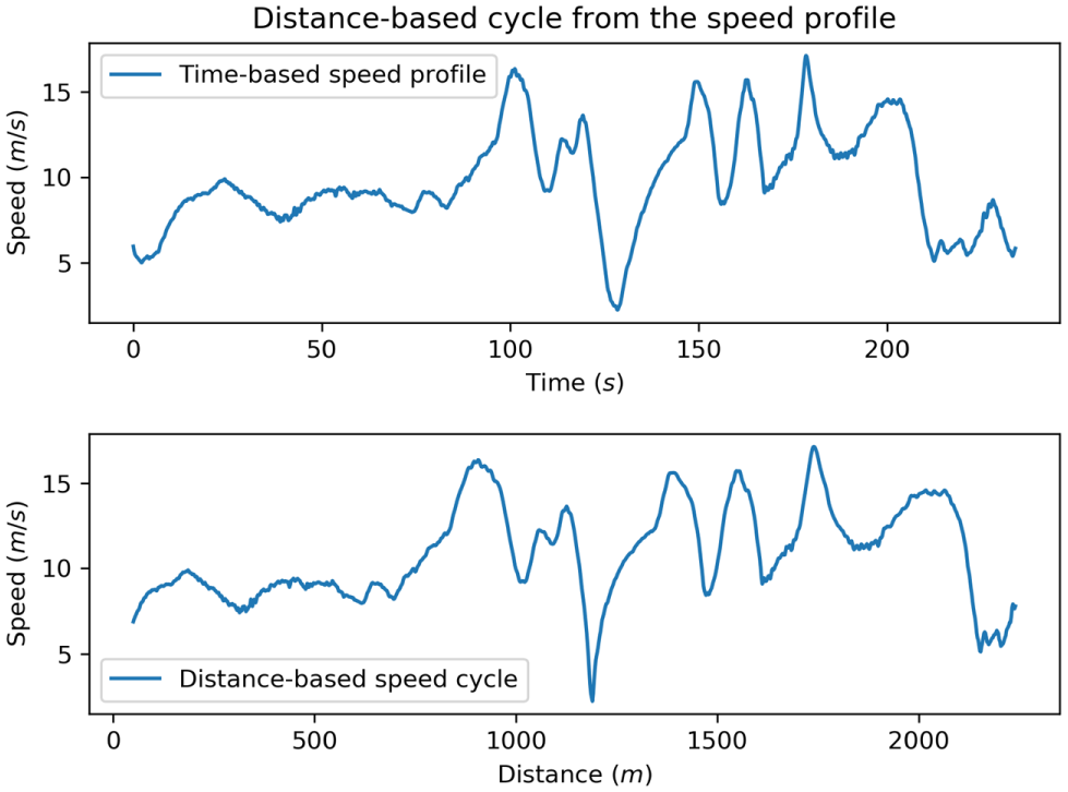
(top) Measured speed-time profile; and (bottom) the corresponding speed-distance cycle.

Gipps Free-Flow Model

Gipps’ model is widely used. In free-flow conditions it assumes that drivers do not exceed their desired speed and that their acceleration decreases with increasing speed:

a_{f} (t) = alpha \cdot a_{n} \cdot (1 - \frac{v_{f} (t)}{V_{f}}) \cdot {(beta + \frac{v_{f} (t)}{V_{f}})}^{gamma}

(10)

where: subscripts f indicates the follower vehicle;

$v (t)$ , and $a (t)$ are the state variables: the vehicle’s speed and acceleration at time t respectively;

$V_{f}$ is the desired speed and $a_{n}$ is the desired acceleration;

Based on the work of Ciuffo et al. ( 30 ), parameter $alpha$ derives automatically from parameters $beta$ and $gamma$ according to the following formula:

alpha = \frac{{(1 + gamma)}^{1 + gamma}}{gamm a^{gamma} \cdot {(1 + beta)}^{1 + gamma}}

(11)

For implementing the free-flow Gipps model, in the case that the desired speed changes and the new value is lower than the current one (and thus the model needs to decelerate) the deceleration of the model is set to the most severe braking equal to $b_{n} = \max (- 2, a_{f} (t))$ .

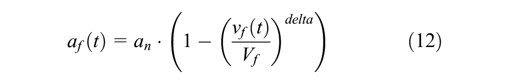
IDM Acceleration Model

IDM is another widely-used model. The free-flow model is computed similarly to the proposed work by Schakel et al. ( 31 ) using the following formula:

a_{f} (t) = a_{n} \cdot (1 - {(\frac{v_{f} (t)}{V_{f}})}^{delta})

(12)

where: subscripts f indicates the follower vehicle;

$v (t)$ , and $a (t)$ are the state variables: the vehicle’s speed and acceleration at time t respectively;

$V_{f}$ is the desired speed and $a_{n}$ is the desired acceleration;

$delta$ is a constant parameter;

For implementing the free-flow model of IDM, similar to the Gipps implementation, the deceleration of the model is set to the most severe braking equal to $b_{n} = \max (- 2, a_{f} (t))$

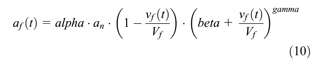
MFC Acceleration Model

MFC is implemented as described in the section above. The free-flow model is computed using the following formula:

a_{f} (t) = a_{w} (v (t)) \cdot a_{cp} (v (t))

(13)

where: subscripts f indicates the follower vehicle;

$v (t)$ , and $a (t)$ are the state variables: the vehicle’s speed and acceleration at time t respectively;

$a_{cp} (v)$ is the acceleration potential of the vehicle, $a_{w}$ is the function that describes the driving style.

As in the other models, the deceleration of the model is set to the most severe braking equal to $b_{n} = \max (- 2, a_{f} (t))$ .

Experimental Results

This section presents the results of this work for the above-mentioned experimental set-up and the three models under test. The assessment of each model refers to its capability to reproduce the measured vehicle dynamics on the road, that is, the vehicle speed and acceleration, at the same point in space (speed over distance cycles). Additional results demonstrate the acceleration capability of each model against official from 0 to 100 km/h acceleration times from a database of over 6,400 vehicles with publicly available technical specifications.

To sum up, the models’ assessment is performed on the following levels:

calibration of the models’ parameters for each experimental lap and validation per lap;

calibration of the models’ parameters on a representative lap and validation on the rest;

validation of the models on official [0–100 km/h] acceleration times; and

discussion around the sensitivity of the models’ parameters.

Calibration on Free-Flow

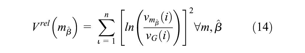
Calibrating a simulation model consists of finding the values of its parameters, allowing the model itself to reproduce in the best possible way the behavior of the real system being simulated. It is equivalent to the solution of a constrained minimization problem in which the objective function expresses the deviation of the simulated measurements from those observed. The calibration in this work is performed based on the global least-squared errors calibration on the sums of squared errors (SSE) discussed in the work of Treiber and Kesting ( 32 ). Similarly, we define the following objective function:

V^{rel} (m_{\hat{β}}) = \sum_{ι = 1}^{n} {[\ln (\frac{v_{m_{\hat{β}}} (i)}{v_{G} (i)})]}^{2} \forall m, \hat{β}

(14)

where

$m$ is a model with its set of parameters $\hat{β}$ ,

$i$ is a distance instance,

$v_{G}$ is the measured speed for the instance $i$ , and

$v_{m_{\hat{β}}}$ is the simulated speed by the model $m$ with parameter vector $\hat{β}$ .

The maximum vehicle speed was under 20 m/s and the simulation step used is 10 Hz, thus, the distance instance was set to 2 m. All comparisons and results refer to every 2-m processing along the predefined path. Since, this work refers to free-flow models there is no interaction with the leader and, consequently, the calibration is performed on the car’s speed. The calibration is performed for each lap and the parameters calibrated per model are shown in the following Table 1.

Table 1.

Parameters Used in Calibration per Model

Model	Parameters
Gipps	$a_{n} \in [0.5, 4], beta \in [0.001, 5], gamma \in [0.5, 4]$
IDM	$a_{n} \in [0.5, 4], delta \in [0.1, 4]$
MFC	$G S_{th} \in [0.1, 1], DS \in [0.1, 1]$

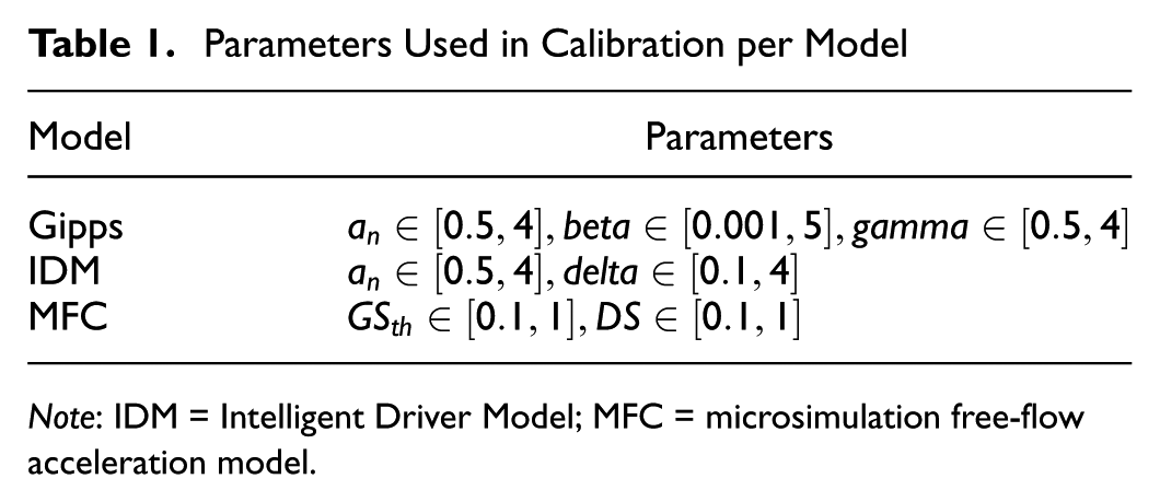
Note: IDM = Intelligent Driver Model; MFC = microsimulation free-flow acceleration model.

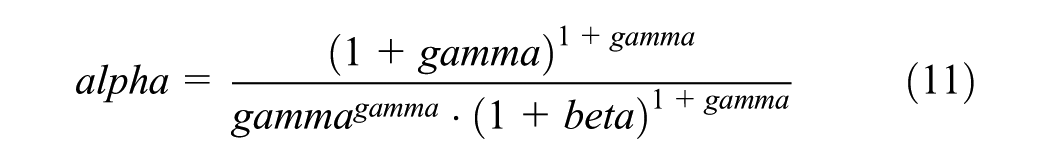
We calibrate beta and gamma, and we compute parameter alpha based on following formulas as stated in the work of Ciuffo et al. ( 30 ):

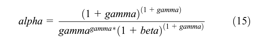
alpha = \frac{{(1 + gamma)}^{(1 + gamma)}}{gamm {a^{gamma}}^{*} {(1 + beta)}^{(1 + gamma)}}

(15)

Figure 8 illustrates the calibrated models and the reference vehicle (GroundTruth) for a part of a lap. The two figures represent the acceleration-distance and speed-distance diagrams of each model, and the final the acceleration-speed diagram for each model. In relation to speed, in general, all three models behave well; Gipps and IDM have very similar behavior making it difficult to spot differences in the figure and both seem to introduce a delay. MFC behaves better staying very close to the reference distance cycle. The most interesting finding is in Figure 8b, where it is obvious that MFC can capture much better the acceleration dynamics of the test vehicle. Gipps and IDM have a much smoother acceleration rate.

Figure 8.

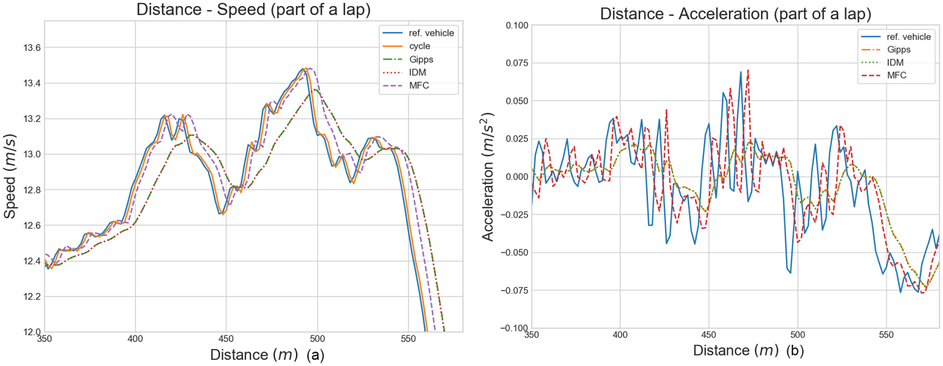
(a) Distance-speed profile, part of a test lap for three models and the test vehicle; (b) the corresponding distance-acceleration profile.

The metrics used for the quantitative results apart from the objective fit function are the following:

Micro Metrics

Root mean square error (RMSE) of the speed.

RMSE of the acceleration.

Macro Metrics

Average speed (and standard deviation) on the total 28 tests.

Average acceleration (and standard deviation) on the total 28 tests.

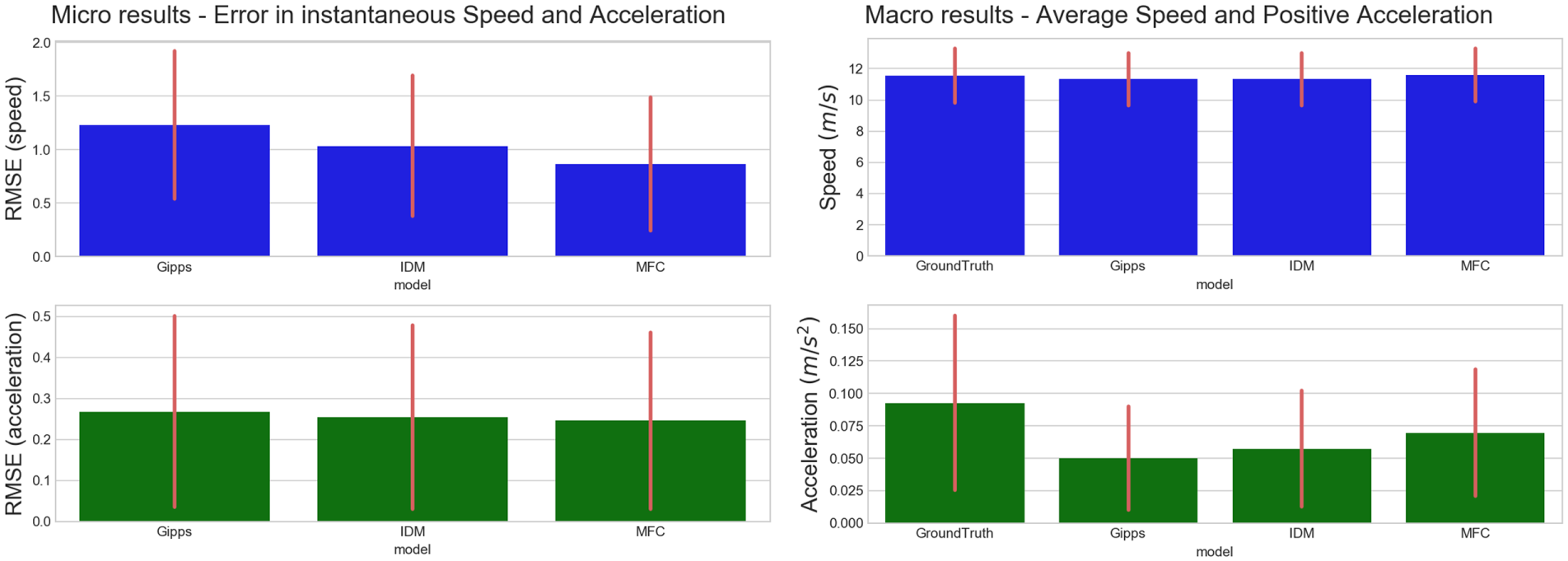
The aggregated results are shown in Figure 9. On a micro level, in average terms over 28 laps, MFC has a much better average fit (Equation 15) with 5.2772, while Gipps and IDM perform similarly with fit values equal to 9.4759 and 9.3573 respectively. The average RMSE of the speed for all laps is around 0.6 m/s for the Gipps and IDM models, while it is almost half for the MFC. The corresponding error for the acceleration is again lower for the MFC, although the difference here is small. In both cases, the standard deviation (red bars) is smaller for MFC than for the other two.

Figure 9.

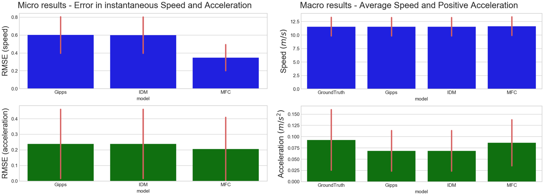
Calibration results: (left) Micro results show the average RMSE for the instantaneous speed and acceleration; and (right) Macro results show the average speed and positive acceleration. The standard deviations for the 28 tests are illustrated by the red bars.

On a macro level, the results presented in Figure 9b refer to the average speed and positive acceleration per lap. Here, the picture is very similar for the speed, with all models being on average very close to the GroundTruth value. However, the average acceleration values for IDM and Gipps are low, while MFC is much closer to the GroundTruth value. This can be explained by the fact that MFC simulates more accurately the vehicle dynamics. It is interesting to see the standard deviation (red bars) in the acceleration of the models, as Gipps and IDM have low values in comparison with the GroundTruth. On the contrary, the standard deviation of the MFC is much closer to the measured one, which means that MFC has a much broader coverage of the acceleration space. Finally, the overall good performance of all three models at the macro level is an indicator that inconsistencies on the instantaneous level are not always visible in the average values.

It is worth mentioning that, initially in the calibration process, the range of values for the parameters, maximum acceleration, alpha, beta, gamma, and delta were much more relaxed. On calibration, it was observed that some parameters tend to fit near the boundaries of the parameters’ value ranges. Maximum acceleration takes very high values (even 10 or 12 m/s² if it is relaxed) for IDM and Gipps that are unrealistic in relation to real vehicle dynamics and, therefore, the parameter loses its physical interpretation. Furthermore, in the case of Gipps, gamma reaches very high values and overfits the model to the calibrated dataset, while beta goes near zero. Per lap test, such extreme values might result in a better fit, but the acceleration-speed diagrams of the model are unrealistic with low generalization power. For example, Figure 10 illustrates the calibrated acceleration-speed diagrams for the three models. The high gamma value in Gipps reduces the acceleration near to zero. This means practically that if the vehicle stops, it cannot start accelerating again. On the other hand, the IDM delta value in some tests reaches very low values close to zero. This reduces the ability of the model to accelerate at high speeds.

Figure 10.

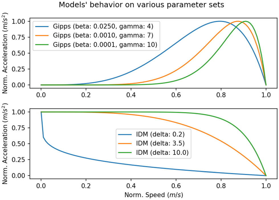
The normalized acceleration-speed curves for the three models.

Validation on Free-Flow

To assess the ability of the models to generalize on calibration, the validation is performed on the basis of the most representative lap. Among the fits of all 28 laps, the one with the median fit values was selected as a representative lap test. The calibrated values of the models for this test were then used for validation in the rest of the 27 laps. The results show that all models perform without increasing their average errors in speed and acceleration. This can be explained from the nature of the experiment, as all tests were performed under very similar conditions. MFC has again a much better average fit (Equation 14), that is 5.7015, while for Gipps and IDM the fit values are 9.6821 and 9.5544 respectively. The conclusions discussed in the calibration section above still hold. Consequently, we can assume that given the same specification of vehicle, driver, weather, and track, all models need few data for calibration.

Validation on Official Vehicle Acceleration Specifications

In addition to the comparison presented above on measured data, this work validates the models on official vehicle specification, in relation to acceleration time from 0 to 100 km/h. A database of around 6,500 commercial cars with their corresponding technical specifications was used to validate all three models. The database refers to vehicles registered after 2012. The vehicles were split into four categories according to their fuel (petrol, diesel) and type of gearbox (automatic, manual).

The scope of the comparison was to validate the models against official specifications and to understand the performance of each model in relation to the vehicle’s power. Table 2 describes the clustering of the vehicles. With reference to the calibration of the models, the parameters alpha, beta, gamma, and delta were set to the default values proposed by the authors (i.e., 2.5, 0.025, 0.5, and 4), the maximum acceleration was set for IDM with the vehicle’s acceleration at 0 km/h, for Gipps the vehicle’s acceleration was set at 32% of the vehicle’s max speed (max acceleration for default parameters) and for MFC the parameters $G S_{th}$ and $DS$ were set to 1 (max value).

Table 2.

Vehicles Clustered in Four Categories Based on their Fuel and Gearbox

Fuel/Gearbox	Manual	Automatic
Petrol	2119	1193
Diesel	1900	1227

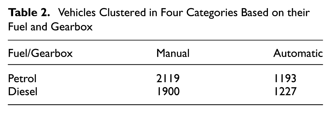
Figure 11 shows the time performance of each model in comparison with the GroundTruth times. The simulated acceleration times of the proposed MFC model are distributed around the diagonal. Furthermore, MFC performs well for all acceleration specs as the error is similar for both lower and higher acceleration times. Gipps and IDM have an overall offset and their error does not seem consistent for all time values. The time deviation seems to grow as the time increases, meaning that both models perform better for faster cars, while for more conservative cars they are very aggressive.

Figure 11.

Comparison of 0–100 km/h acceleration time per model against the official acceleration time.

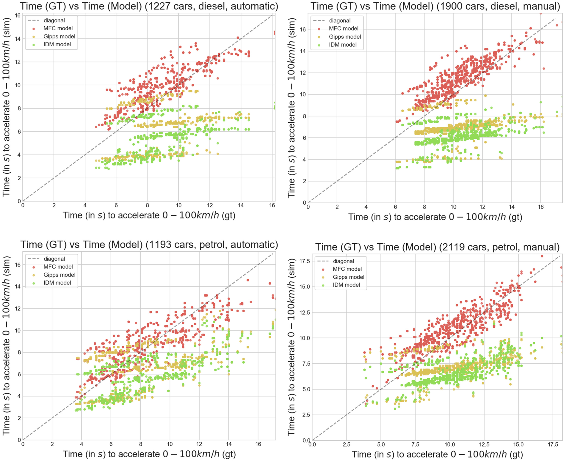
Figure 12 shows the performance of each model across the engine power range. Once more, the MFC times are much closer to the GroundTruth distribution, while Gipps and IDM face a growing, non-consistent error. Gipps and IDM models perform better for vehicles with higher engine power.

Figure 12.

0–100 km/h acceleration time per model over the vehicle’s engine power for the four vehicle categories.

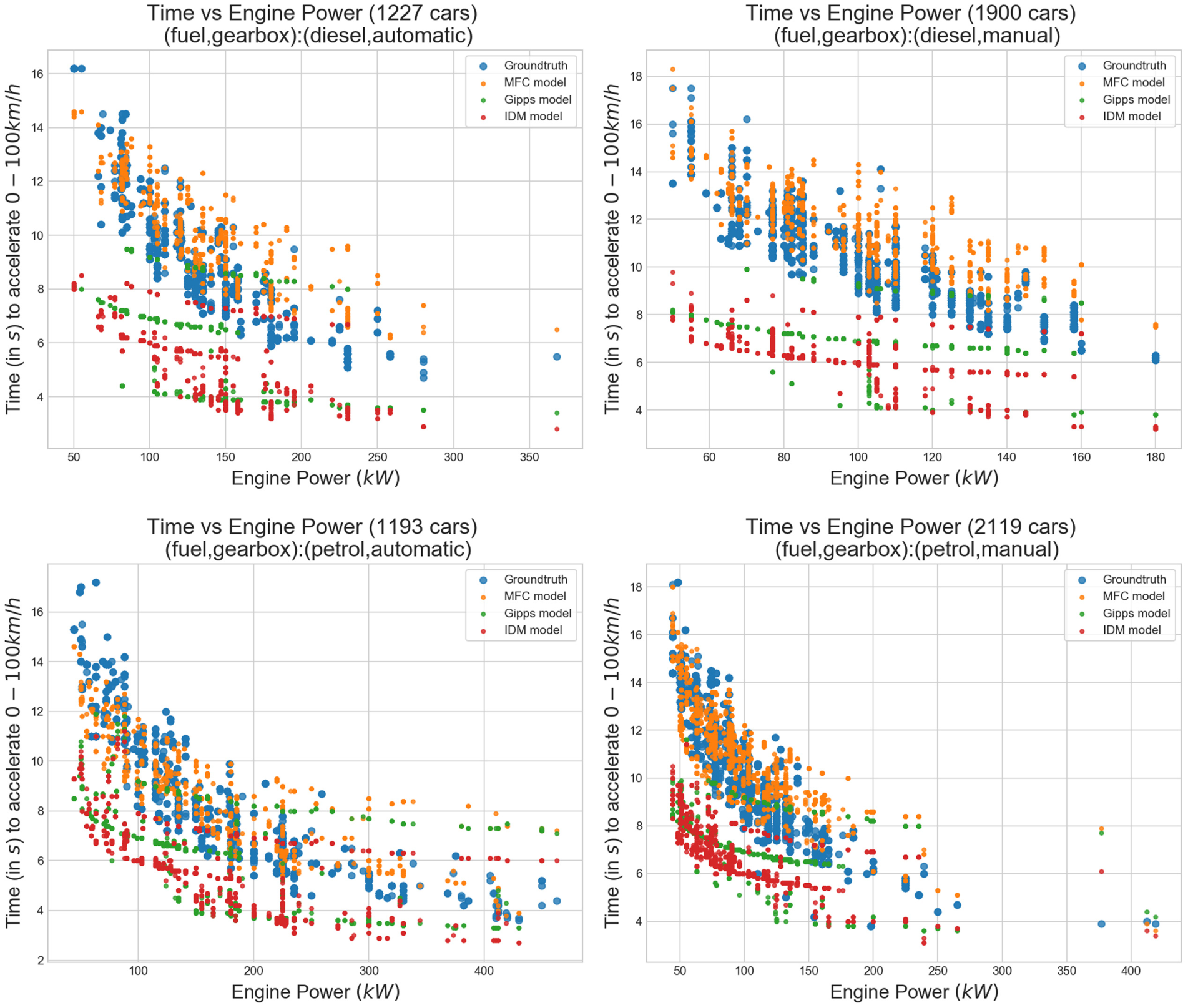
Finally, Figure 13 shows the distribution of time errors. The results confirm once more, the observations from the previous figures. The peak in the MFC distribution is higher, and the accuracy/precision values better than the other two models.

Figure 13.

Distribution of time error per model per vehicle category.

Sensitivity of the Model Parameters

This last section aims to test the sensitivity of the maximum acceleration parameter for each model, to see if the error of each model is consistent across different acceleration values.

We perform for each model, for each lap, three simulations with different maximum acceleration values, ${\max (a_{i, lap}) - 2, \max (a_{i, lap}), \max (a_{i, lap}) + 2}$ , where $\max (a_{i, lap})$ is the maximum acceleration observed at instance $i$ for the specific test lap. We fix alpha, bets, gamma, and delta parameters to the values proposed in the original works, that is, 2.5, 0.025, 0.5, and 4. Since MFC does not have a maximum acceleration parameter, to create a fair comparison, we introduce the following relationship between the maximum acceleration parameter in Gipps and IDM and the $DS$ parameter in the MFC.

More specifically:

DS = \frac{\max (a_{i, lap})}{\max (a_{cp})}

(16)

The $G S_{th}$ parameter is set equal to $DS$ .

The results in Figure 14 show the robustness of the MFC in variations of the maximum acceleration parameter. The fit error values are much higher as expected, yet MFC has a better average fit value with 17.5941 over the ones from Gipps and IDM (28.9059 and 21.7766 respectively). MFC performs better on the RMSE in speed and acceleration; Gipps seems to have the biggest error of the three models.

Figure 14.

Sensitivity results: (left) micro results show the average RMSE for the instantaneous speed and acceleration; and (right) macro results show the average speed and positive acceleration. The standard deviations for the 28 tests are illustrated by the red bars.

Conclusions

The present work proposes the MFC vehicle free-flow model, that is able to capture the vehicle acceleration dynamics in an accurate and consistent way, provides a link between the model and the driver, and can be easily implemented and tested in microsimulation software without raising the computational complexity. The MFC free-flow part can be also used in an existing model by substituting their corresponding part. The model is calibrated, validated, and compared with known car-following models on road data on a fixed route inside the Joint Research Centre of the European Commission. Finally, MFC is assessed on 0–100 km/h acceleration specifications of vehicles available in the market. The results prove the robustness and flexibility of the model.

Some advantages of the MFC are that it:

captures with improved accuracy and precision the vehicle acceleration dynamics;

creates links between car-following behavior, the vehicle, and the driver;

ensures minimal additional complexity;

provides additional instantaneous info such as gear and engine rpm;

facilitates the use of instantaneous emissions models;

characterizes the driver style offering the potential for driver-related studies;

offers the possibility of building a realistic fleet composition of passenger vehicles;

offers a more accurate representation of human driving which is necessary for mixed scenarios with human-driver and autonomous vehicles.

MFC can be further extended and improved in various ways, but it is considered that this work opens the way to using vehicle dynamics in extended microsimulation studies. For future work and improvement, some of the possible steps could be: (1) assessment of the model with regard to instantaneous emissions calculation; (2) impact assessment of vehicle dynamics over a complex network in relation to both flow and emissions; (3) the design of a more refined and realistic gear-shifting logic; (4) the design and implementation of a realistic car-following and deceleration logic toward a complete vehicle dynamics-based driver model; and (5) expansion of the model for hybrids and electric cars.

Footnotes

Acknowledgements

The authors acknowledge the JRC Vehicle Emissions Laboratory (VELA) team for their support during the whole experimental activity described in the present study.

Author Contributions

The authors confirm contribution to the paper as follows: study conception and design: all authors; data collection: all authors; analysis and interpretation of results: all authors; draft manuscript preparation: all authors. All authors reviewed the results and approved the final version of the manuscript.

The Standing Committee on Traffic Flow Theory and Characteristics (AHB45) peer-reviewed this paper (19-04093).

The views expressed here are purely those of the authors and may not, under any circumstances, be regarded as an official position of the European Commission.

References

Brackstone

McDonald

Car-Following: A Historical Review. Transportation Research Part F: Traffic Psychology and Behaviour, Vol. 2, No. 4, 1999, pp. 181–196. https://doi.org/10.1016/S1369-8478(00)00005-X.

Helbing

Traffic and Related Self-Driven Many-Particle Systems. Reviews of Modern Physics, Vol. 73, No. 4, 2001, pp. 1067–1141. https://doi.org/10.1103/RevModPhys.73.1067.

Cao

Yang

Car-Following Models Study Progress. IEEE Computer Society, Washington, D.C., 2009.

Zheng

Suzuki

Fujita

Evaluation of Car-Following Models Using Trajectory Data from Real Traffic. Procedia - Social and Behavioral Sciences, Vol. 43, 2012, pp. 356–366. https://doi.org/10.1016/j.sbspro.2012.04.109.

Gazis

D. C.

Herman

Rothery

R. W.

Nonlinear Follow-the-Leader Models of Traffic Flow. Operations Research, Vol. 9, No. 4, 1961, pp. 545–567.

Gipps

P. G.

A Behavioural Car-Following Model for Computer Simulation. Transportation Research Part B: Methodological, Vol. 15, No. 2, 1981, pp. 105–111. https://doi.org/10.1016/0191-2615(81)90037-0.

Newell

G. F.

A Simplified Car-Following Theory: A Lower Order Model. Transportation Research Part B: Methodological, Vol. 36, No. 3, 2002, pp. 195–205. https://doi.org/10.1016/S0191-2615(00)00044-8.

Bando

Hasebe

Nakayama

Shibata

Sugiyama

Dynamical Model of Traffic Congestion and Numerical Simulation. Physical Review E, Vol. 51, No. 2, 1995, pp. 1035–1042. https://doi.org/10.1103/PhysRevE.51.1035.

Nagel

Schreckenberg

A Cellular Automaton Model for Freeway Traffic. Journal de Physique I, Vol. 2, No. 12, 1992, pp. 2221–2229. https://doi.org/10.1051/jp1:1992277.

10.

Marczak

Leclercq

Buisson

A Macroscopic Model for Freeway Weaving Sections. Computer-Aided Civil and Infrastructure Engineering, Vol. 30, No. 6, 2015.

11.

Ciuffo

Makridis

Toledo

Fontaras

Capability of Current Car-Following Models to Reproduce Vehicle Free-Flow Acceleration Dynamics. IEEE Transactions on Intelligent Transportation Systems, 2018, pp. 1–10. https://doi.org/10.1109/TITS.2018.2866271.

12.

Lejri

Can

Schiper

Leclercq

Accounting for Traffic Speed Dynamics When Calculating COPERT and PHEM Pollutant Emissions at the Urban Scale. Transportation Research Part D: Transport and Environment, Vol. 63, 2018, pp. 588–603. https://doi.org/10.1016/j.trd.2018.06.023.

13.

Galvin

Energy Consumption Effects of Speed and Acceleration in Electric Vehicles: Laboratory Case Studies and Implications for Drivers and Policymakers. Transportation Research Part D: Transport and Environment, Vol. 53, 2017, pp. 234–248. https://doi.org/10.1016/j.trd.2017.04.020.

14.

Ahn

Rakha

Trani

Van Aerde

Estimating Vehicle Fuel Consumption and Emissions Based on Instantaneous Speed and Acceleration Levels. Journal of Transportation Engineering, Vol. 128, No. 2, 2002, pp. 182–190. https://doi.org/10.1061/(ASCE)0733-947X(2002)128:2(182).

15.

Zhang

Wang

Evaluation of Vehicle Acceleration Models for Emission Estimation at an Intersection. Transportation Research Part D: Transport and Environment, Vol. 18, 2013, pp. 46–50. https://doi.org/10.1016/j.trd.2012.09.004.

16.

Jeong

Lee

Emission Evaluation of Inter-Vehicle Safety Warning Information Systems. Transportation Research Part D: Transport and Environment, Vol. 41, 2015, pp. 106–117. https://doi.org/10.1016/j.trd.2015.09.018.

17.

Madireddy

De Coensel

Can

Degraeuwe

Beusen

De Vlieger

Botteldooren

Assessment of the Impact of Speed Limit Reduction and Traffic Signal Coordination on Vehicle Emissions Using an Integrated Approach. Transportation Research Part D: Transport and Environment, Vol. 16, No. 7, 2011, pp. 504–508. https://doi.org/10.1016/j.trd.2011.06.001.

18.

Xie

Chowdhury

Bhavsar

Zhou

An Integrated Modeling Approach for Facilitating Emission Estimations of Alternative Fueled Vehicles. Transportation Research Part D: Transport and Environment, Vol. 17, No. 1, 2012, pp. 15–20. https://doi.org/10.1016/j.trd.2011.08.009.

19.

Stevanovic

Zhang

Batterman

Optimizing Traffic Control to Reduce Fuel Consumption and Vehicular Emissions. Transportation Research Record: Journal of the Transportation Research Board, 2009. 2128: 105–113.

20.

Boriboonsomsin

Barth

Impacts of Freeway High-Occupancy Vehicle Lane Configuration on Vehicle Emissions. Transportation Research Part D: Transport and Environment, Vol. 13, No. 2, 2008, pp. 112–125. https://doi.org/10.1016/j.trd.2008.01.001.

21.

Smit

Development and Performance of a New Vehicle Emissions and Fuel Consumption Software (PΔP) with a High Resolution in Time and Space. Atmospheric Pollution Research, Vol. 4, No. 3, 2013, pp. 336–345. https://doi.org/10.5094/APR.2013.038.

22.

Ericsson

Independent Driving Pattern Factors and Their Influence on Fuel-Use and Exhaust Emission Factors. Transportation Research Part D: Transport and Environment, Vol. 6, No. 5, 2001, pp. 325–345. https://doi.org/10.1016/S1361-9209(01)00003-7.

23.

Toffolo

Morello

Samaras

Ntziachristos

Vock

Maier

Garcia-Castro

ICT-Emissions Methodology for Assessing ITS and ICT Solutions. Proc., 5th Conference on the Transport Research Arena (TRA): Transport Solutions from Research to Deployment, Paris, 2014.

24.

Rakha

Snare

Dion

Vehicle Dynamics Model for Estimating Maximum Light-Duty Vehicle Acceleration Levels. Transportation Research Record: Journal of the Transportation Research Board, 2004. 1883: 40–49.

25.

Karim

Rakha

Loulizi

Abdelkefi

Vehicle Dynamics Model for Estimating Typical Vehicle Accelerations. Transportation Research Record: Journal of the Transportation Research Board, 2015. 2491: 61–71.

26.

Rakha

H. A.

Ahn

Faris

Moran

K. S.

Simple Vehicle Powertrain Model for Modeling Intelligent Vehicle Applications. IEEE Transactions on Intelligent Transportation Systems, Vol. 13, No. 2, 2012, pp. 770–780. https://doi.org/10.1109/TITS.2012.2188517.

27.

Aimsun Next. Transport Simulation Systems. https://www.aimsun.com. Accessed December 19, 2016.

28.

Treiber

Hennecke

Helbing

Congested Traffic States in Empirical Observations and Microscopic Simulations. Physical Review E, Vol. 62, No. 2, 2000, pp. 1805–1824. https://doi.org/10.1103/PhysRevE.62.1805.

29.

Tsiakmakis

Fontaras

Ciuffo

Samaras

A Simulation-Based Methodology for Quantifying European Passenger Car Fleet CO₂ Emissions. Applied Energy, Vol. 199, 2017, pp. 447–465. https://doi.org/10.1016/j.apenergy.2017.04.045.

30.

Ciuffo

Punzo

Montanino

Thirty Years of Gipps’ Car-Following Model: Applications, Developments, and New Features. Transportation Research Record: Journal of the Transportation Research Board, 2012. 2315: 89–99.

31.

Schakel

W. J.

van Arem

Netten

B. D.

Effects of Cooperative Adaptive Cruise Control on Traffic Flow Stability. Proc., 13th International IEEE Conference on Intelligent Transportation Systems, Madeira Island, Portugal, IEEE, 2010, pp. 759–764.

32.

Treiber

Kesting

Microscopic Calibration and Validation of Car-following Models – A Systematic Approach. Procedia - Social and Behavioral Sciences, Vol. 80, 2013, pp. 922–939. https://doi.org/10.1016/j.sbspro.2013.05.050.

MFC Free-Flow Model: Introducing Vehicle Dynamics in Microsimulation

Abstract

MFC Free-Flow Model Description

The Acceleration-Speed Curve of the Vehicle

Gear-Shifting Strategy

Driving Style

Driver’s Acceleration-Speed Profile

Implementation of the MFC in Microsimulation

Experimental Set-Up

Gipps Free-Flow Model

IDM Acceleration Model

MFC Acceleration Model

Experimental Results

Calibration on Free-Flow

Micro Metrics

Macro Metrics

Validation on Free-Flow

Validation on Official Vehicle Acceleration Specifications

Sensitivity of the Model Parameters

Conclusions

Footnotes

Acknowledgements

Author Contributions

References