
Abstract
This paper studies the activity profiles of truck drivers in urban areas. Finding repeating dynamical patterns is important in understanding freight behaviors, and aids freight-friendly planning. In the digital age, data on truck drivers is becoming more available with heterogeneous demographic and work profiles. By synthesizing such pervasive data and applying machine learning concepts, this paper proposes to identify signature travel activity patterns via dimensionality reduction. Based on driver survey data, truck drivers’ behaviors are represented as longitudinal activity sequences. Dimensionality reduction and activity reconstruction via principal components analysis (PCA), logistic PCA, and autoencoder were conducted to reveal fundamental activity features and approximate the underlying data-generating function. In the driver survey dataset, 243 truck drivers in Singapore reported their daily activities for 1,099 weekdays. This study found that PCA produced the most faithful reconstruction of drivers’ activities. When projecting the input data down from 2,592 to 82 dimensions, PCA explained 77% of variances with a reconstruction error of 0.99%. Logistic PCA is a useful extension of PCA to study the pattern of a single activity. It captures the variation of infrequent activities such as truck queuing, which PCA fails to reconstruct. Autoencoder was found to be more powerful than PCA in reconstructing activities – with 1% of original dimensions, it reconstructed the activities with an error rate of 1.24%. Moreover, when implemented as a variational autoencoder, autoencoder generated realistic-looking samples of driver activities. The top three most distinctive activity patterns of Singapore truck drivers are reported using PCA.
Passenger and freight transportation systems vary fundamentally, therefore, different types of models have been developed to study their respective travel behaviors. For passenger mobility, different modeling frameworks, such as the traditional four-step travel demand model, are readily available. Household travel surveys are used to collect data for these models. In recent years, pervasive sensing has provided a novel data source to study passenger travel behaviors. At the same time, advances in data mining have also inspired new analytical frameworks for studying the dynamics of passenger activities (1–4). Freight travel, however, is less well researched due to scarcity of freight data, the involvement of multiple decision makers and supply chain actors, and complexity in modeling. In modeling travel behaviors, freight agents are more heterogeneous and their behaviors vary more than passengers. For example, a typical passenger’s day may consist of a few key locations such as home, school, or work, whereas a truck driver can visit dozens of locations and perform different activities in a day. Consequently, characterizing activity patterns of freight travel is less intuitive and straightforward than doing so for passenger travel.
This study set out to explore the activity profiles of truck drivers in cities. To address the first issue of the lack of freight data, GPS tracking and a stop-based driver survey were conducted to capture the activities that truck drivers performed at each stop over several days. Because a truck driver typically visits many locations and engages in multiple activities daily, such as pickups or deliveries, the corresponding activity profile requires a high-dimensional representation. Therefore aggregation of information is needed to discover meaningful activity patterns while preserving critical details of the activity profiles. Tour-based models are important approaches in studying freight behaviors ( 5 , 6 ). To complement these models, this paper proposes a framework in which patterns are extracted automatically without a priori knowledge on how truck drivers should behave.
Inspired by Eagle and Pentland’s pioneering work in which principal components analysis (PCA) was first used to analyze human mobility patterns ( 2 ), this paper proposes a methodology framework where dimensionality reduction is used to identify activity patterns. The central idea of this approach is to represent the high-dimensional activity sequence in lower dimensions while retaining the essential information. By forcing a model to prioritize which aspects of the input activity data to keep in lower dimension, it often learns key features of the original activities ( 7 ). From the lower-dimension representation, travel activities can be reconstructed. The discrepancy between the reconstruction and the original activity sequences is used as the main metric for evaluating how well the lower-dimension representation preserves the inherent structure of the observed behavior. In the proposed framework, dimensionality reduction techniques of PCA, logistic PCA, and autoencoder are implemented independently. Using high-resolution real-life freight activity data, their performances on discovering underlying patterns in truck driver activities are evaluated.
In line with this objective, the contribution of this paper is twofold. First, in terms of methodology, it provides novel implementations of logistic PCA, autoencoder, and variational autoencoder (VAE) in uncovering the inherent travel activity patterns. Although PCA has been applied in human mobility research ( 2 , 4 , 8 ), other dimensionality reduction techniques such as autoencoder, which are widely used in image processing, natural language processing and representation learning are almost never implemented in detecting mobility patterns. This paper develops practical implementations of these four techniques in analyzing freight activity patterns, and compares their performance. Second, from an empirical perspective, this study exposes the fundamental heterogeneity in urban truck drivers’ activity sequences by applying dimensionality reduction to a large dataset collected from 243 truck drivers in Singapore. Due to scarcity of data, few studies have comprehensively described freight activities at an aggregate level. The patterns identified from this dataset provide evidence on the existence of distinct and repeating activity chains in urban freight transport.
The remainder of this paper is organized as follows. Section 2 describes the dataset used, and the data transformation methodology. In section 3, PCA, logistic PCA, autoencoder, and VAE are introduced. Section 4 presents the best model from each of the dimensionality reduction methods described in section 3 when applied to the input dataset. The validity of these four methods is discussed. Section 5 describes the Singapore truck drivers’ activity patterns discovered from the dataset. Finally, this paper concludes with comparisons on methods developed, their significance, and application for future work.
Data
Data Description
The sample data used in this study orginates from an ongoing freight vehicle survey in Singapore. Using a fully digital data collection platform – Future Mobility Sensing-Freight (FMS-Freight) – truck and driver activity data of high granularity was acquired ( 9 ). For each truck driver participating in the survey, a GPS logger was installed in the vehicle that continuously collected the vehicle’s location data. Based on the raw logger data, as well as other contextual information (e.g., land use, points of interest etc.), FMS-Freight inferred drivers’ stop times, locations, and activities. The driver is presented with the inferred timeline in a web interface, in which they can verify the details and answer additional questions such as stop location functions, commodity type, shipment volume, and so forth. Each driver was required to verify the activities performed for five consecutive weekdays. The data collection project started in February 2017 and aimed to track over 6,000 truck drivers.
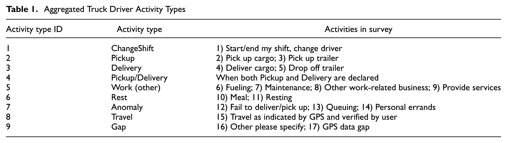
At the time this paper was produced, only data on heavy goods vehicles were available, which are trucks with a maximum laden weight of more than 3,500 metric tons. After removing activity data that was either incomplete or with missing GPS information, a dataset with a total of 1,099 weekdays of activities reported by 243 heavy goods vehicle drivers was used as the input. Among the 243 drivers, 62% worked in the construction industry, followed by 13% in manufacturing and 9% in transportation and storage. Among the 243 vehicles operated by drivers, 213 were heavy goods vehicles. In the remaining 30 non-goods vehicles, there were 24 prime movers, three cranes, two concrete mixers and a recovery vehicle. Activity options posed in the survey questionnaire are presented in Table 1.
Aggregated Truck Driver Activity Types
Data Transformation
In studying a truck driver’s activities, a suitable representation of an activity sequence from the raw survey data is needed. Two possible approaches have been reported in the literature: 1) represent an activity sequence as a vector
Using the same notation as in Jiang et al. ( 4 ), each day was divided into a total of 288 time intervals, each with a 5 min interval duration. For each individual driver, the activity occurring at the first second of a time interval would be noted as the activity for the entire time interval.
Let G be the total number of activity types. Jiang et al. propose the G activities satisfy the “compatibility condition” before applying PCA ( 4 ). This condition requires that at any given time interval, a driver should engage in one – and only one – activity. Jiang et al.’s rationale is mainly driven by the need for the multivariate Gaussian assumption of applying PCA. Their reconstruction method is also based on their formulation of an activity sequence in which each time interval corresponds to only one activity type ( 4 ). For logistic PCA, the compatibility condition can be relaxed due to its Bernoulli probability assumption; therefore, it allows multiple activities to happen within the same time interval. For autoencoder and VAE, although the compatibility condition is not required, the same input as with PCA is used for comparison.
Formally, an activity sequence
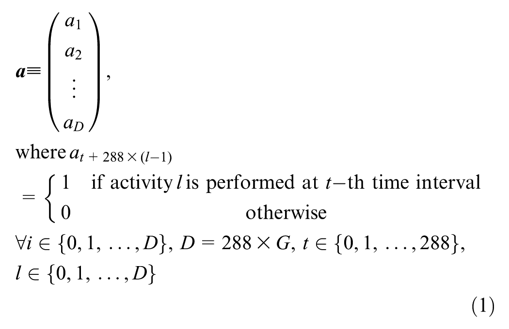
The space of individuals’ daily behaviors can thus be defined as the matrix space
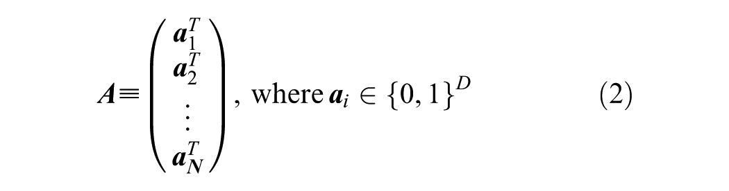
In the dataset, each driver could select multiple activities at the same stop. However, when the compatibility condition is binding, activities are aggregated into G = 9 types in Table 1. A main activity is assigned to each interval. The activity with a smaller ID would be used as the main one. Without the compatibility condition, each interval can have multiple activities. Activities are aggregated into G = 8 types, excluding “Pickup/Delivery” in Table 1.
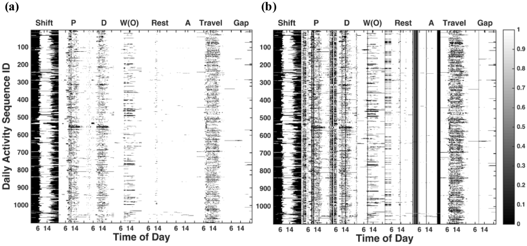
By counting the percentage of drivers performing each of the G activities in Table 1, the temporal rhythm of truck drivers’ activities can be revealed. Figure 1a depicts the variation in truck drivers’ activities on an average weekday. It describes the average percentage of drivers engaging in a specific activity at any given time in a weekday. Drivers begin their work shift around 6:00 a.m., and the number increases rapidly until 10:00 a.m. What accompanies this trend in the start of the shifts is traveling (driving). As expected, drivers start traveling around the same time when they start their shift. After 3:00 p.m., drivers begin to end their shift and this continues until 12:00 a.m., suggesting that the end-shift time varies greatly across drivers.
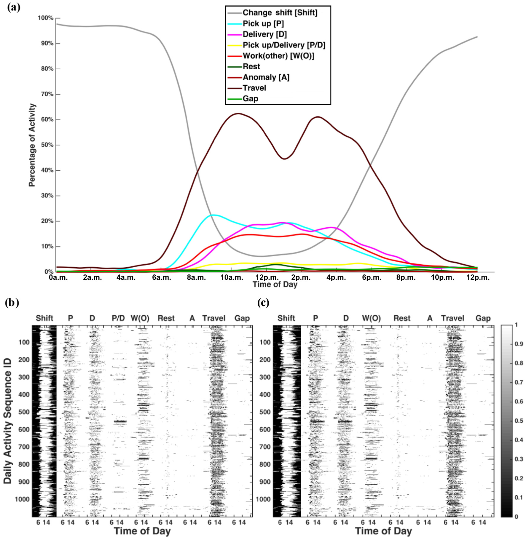
(a) aggregated temporal variation of 243 truck drivers’ activities on an average weekday; (b) activity matrix when G = 9; (c) activity matrix when G = 8.
Approximately 30 min after traveling, “Pickup” activity increases, followed by “Work(other)” and “Delivery.” As service trips are categorized under “Work(other),” it could be the case that service trucks start working later than cargo-carrying ones. Around 12:00 p.m., drivers reduce their traveling and the number of “Rest” entries start to peak. This implies that, although not many drivers rest during a shift, if they do it tends to be around noon. In the afternoon, “Pickup” declines before “Work(other)” and “Delivery,” which is consistent with the morning trend. Overall, “Pickup” activities have two peaks during the day, one around 9:00 a.m. and another at 1:00 p.m. Similar trends held for “Delivery,” but happened at later time intervals. “Anomaly” and “Gap” had a small presence in the dataset, and their occurrences were observed to be independent of the time of day.
Following the notation in Equation 1 and Equation 2, the input dataset for dimensionality reduction is visualized in Figure 1, b and
c
as black-and-white images. For
Methodology
Related Work
PCA was first used to extract mobility patterns from human activities (Eagle and Pentland [ 2 ]). Over 100 subjects’ daily activities were reconstructed using six primary characteristic vectors, termed “eigenbehaviors,” with an accuracy of 90%. Their method can be generalized into the framework described below:
Define the activity space of all sample subjects as a matrix
Represent the activity matrix in a lower-dimension matrix
Reconstruct the activity data as
Step 1 transforms the dataset into activity sequences as denoted in Equation 1 and Equation 2; whereas Step 2 performs dimensionality reduction on the transformed data obtained in Step 1. Depending on which dimensionality reduction method is used in Step 2, activity reconstruction in Step 3 will vary. Currently, PCA is the main technique used to analyze human mobility patterns ( 2 , 4 , 8 ). However, because of the fundamental differences between freight and passenger activities, PCA may not have been the most suitable for the truck driver activity dataset used in this paper. Logistic PCA, autoencoder, and VAE were therefore explored because they had more relaxed probabilistic assumptions on the input variables.
The idea behind the work of Eagle and Pentland is widely applied in fields such as image processing, bioinformatics, and natural language processing (2, 8–10). Pattern, or feature discovery via dimensionality reduction is an important problem in representation learning. Intuitively, what happens during dimensionality reduction is that more “noisy” data is thrown out so that what remains is more relevant in representing the key features. By assuming there exists some underlying structure in an activity sequence or behavior space, dimensionality reduction can uncover this structure by also removing the noise. Jiang et al. document a step-by-step implementation of PCA in revealing passenger activity patterns ( 4 ). This paper applied the same PCA method to examine truck driver activity patterns, and expanded the framework to incorporate other dimensionality reduction methods: logistic PCA, autoencoder, and VAE. As all three methods are well developed, the contribution of this paper in implementing them in activity pattern discovery mainly lies in activity reconstruction. The formulation of PCA follows the work of Pearson ( 11 ); whereas the formulation of logistic PCA used is from Landgraf and Lee ( 12 ). As Tensorflow is used to implement autoencoder and VAE, their formulation follows those incorporated in Tensorflow ( 13 ).
Logistic PCA and autoencoder were selected as comparisons to PCA mainly because these three methods were compared in performing similar tasks. Hinton and Salakhutdinov compared the performance of PCA, logistic PCA, and autoencoder in learning the lower-dimensional representation of high-dimensional data ( 10 ). The data used in their work was randomly chosen from the MNIST dataset ( 12 ) of handwritten digits. Using Hinton and Salakhutdinov’s method of training deep autoencoder networks, autoencoder produced a much clearer reduced image than PCA and logistic PCA ( 10 ). The standard autoencoder can be implemented as a variational autoencoder, which is a popular approach not only in dimensionality reduction, but also in generating new information ( 14 ).
In evaluating the performance of pattern discovery via different dimensionality reduction methods, one important diagnostic metric is reconstruction error. This is defined as the percentage of incorrectly reconstructed entries out of the total number of entries. Let

A low reconstruction error means the reconstruction is a truthful representation of the original activity data. However, a reconstruction error of zero is not desirable, because a model learns nothing useful about an input by copying it. To address this issue, another diagnostic metric in selecting the best method is the intermediate dimensions, that is, K (see next section). The goal is to maintain a relatively faithful reconstruction of the input data while minimizing the number of intermediate dimensions. Furthermore, in the context of freight behavior research, interpretability of the output is equally important.
PCA
PCA has been widely used as a dimensionality reduction technique ( 15 ). From its mathematical formulation, PCA finds the optimal representation of multivariate data in lower dimensions by minimizing the mean squared error (MSE). PCA thus possesses an appealing geometric property: it is a linear projection in which high-dimensional data is projected into a lower-dimensional space. Following Jiang et al. ( 4 ), applying PCA to reconstruct travel activity was formally formulated as below.
Let
Let
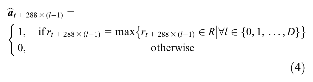
Compute
For any t∈{1, 2,…,288}, l∈{1, 2,…,G}.
Logistic PCA
Similar to PCA, the geometric interpretation of logistic PCA is also a projection, but nonlinear.
Dissimilar from PCA, logistic PCA assumes that each element

After obtaining principal components using logistic PCA, activities can be reconstructed as follows.
Let
Let
Compute
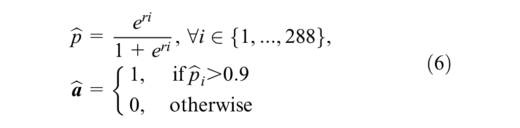
Select a probability threshold h = 0.9.
Autoencoder and Variational Autoencoder (VAE)
Autoencoder reduces dimensionality via stacked layers of feedforward networks. Conceptually, an autoencoder is an unsupervised representation of original data. It generally learns the identity function F(X) = X under the constraint on dimensionality ( 7 ). The advantage of autoencoder is that it can result in powerful outcomes because neural networks are universal function approximators (19–21). However, it also suffers from the typical problem of feedforward networks: results are not readily interpretable. Tensorflow was used to develop autoencoder models in this paper; Python codes, used to train the model, is available on GitHub at https://github.com/urbanfreight/Dimensionality-Reduction. The activity reconstruction was performed as below.
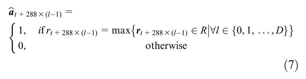
Let
VAE is one type of autoencoder that learns the latent variable space of its input data. Whereas autoencoder learns to approximate the input, VAE learns the parameters of the probability distribution that generates the input. VAE was defined in 2013 by Kingma and Welling ( 14 ) and has been widely applied in the top-performing models in image generation and reinforcement learning ( 18 ).
Implementation and Results
This section presents findings from employing the four machine learning methods introduced. For each method, the parameter selection process is described and the reconstruction yielded by the best model is presented. The validity of applying each method to analyze truck driver activities is discussed.
PCA
Due to the compatibility condition, the input dataset selected for PCA consisted of nine activity types, as shown in Figure 1a. At any given time in a day, a driver can engage in one of the nine activity types. PCA requires one parameter to reconstruct the input dataset: K, the number of eigenvectors. Geometrically, K also represents the number of dimensions the original input is projected to.
In selecting K, two measures were used: 1) the percentage of variance explained; 2) the reconstruction error. In Figure 2a, the left panel shows that the percentage of variance explained increases with K; the right panel indicates that the reconstruction error reduces when K increases.
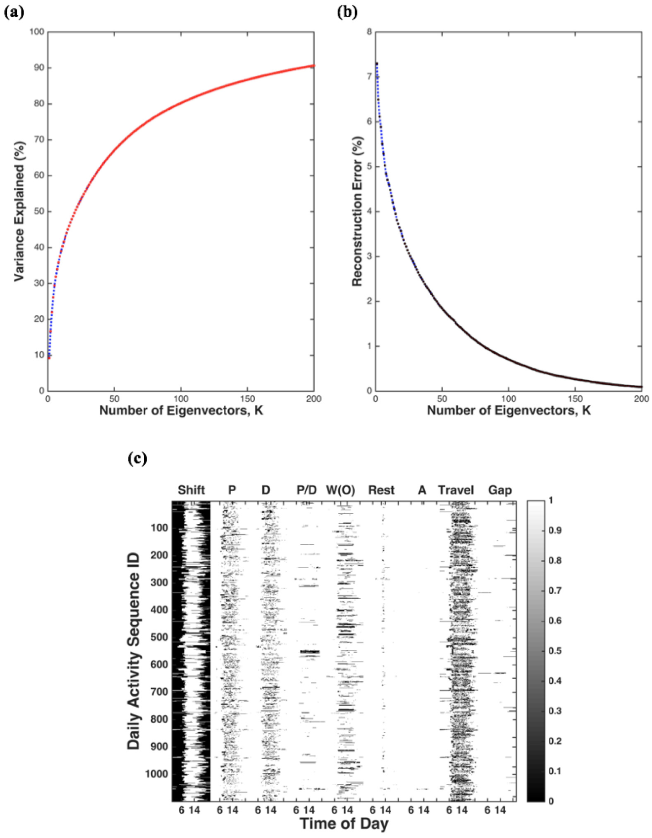
PCA: (a) percentage of variance explained; (b) reconstruction error; (c) the reconstruction matrix with K = 82.
At K = 82, the reconstruction error drops to 0.99%. The percentage of variance explained is 77%. Figure 2b shows the reconstruction matrix, which provides a faithful reconstruction of the input except for “Anomaly” activity type. When applying the same method to the Chicago Household Travel Survey, Jiang et al. used only 21 eigenvectors to reconstruct 99% of the original weekday activities ( 4 ). The different results the same method yields when applied on passenger and freight activity datasets suggests that freight activities are inherently less regular and thus less predictable than passenger activities.
Logistic PCA
Logistic PCA assumes that the input data is binary, and each element in the input activity matrix comes from a Bernoulli distribution. If all activities were used as input at the same time, then it assumes that these activities are independent events, which clearly is not the case. For example, if a driver declared “Pickup,”“Deliver” is expected at some later time interval. Therefore, when applying logistic PCA to reconstruct the input activities, the reconstruction is performed activity by activity. Specifically, the input activity matrix shown in Figure 1b is split into eight smaller activity matrices, with each representing one of the eight activity types. Logistic PCA is employed to reconstruct each of the smaller activity matrices.
Two parameters are required before reconstructing with logistic PCA: m and K. The first parameter m, whose true value is defined in Equation 5, is selected to maximize the log likelihood of generating the input matrix. The R-package “logisticPCA” developed by Landgraf and Lee is used to select m ( 16 ). After m is determined, K is selected to explain 90% of variances. With m and K, principal components and scores can be computed and reconstruction can then be performed. Combining the best models for each activity type, the total number of eigenvectors used in the reconstruction was 93. By setting the probability threshold, h = 0.9, the reconstruction error was 3.21%. When h = 0.5, the reconstruction error rose to 7.31%. Figure 3, a and b show the two reconstructed matrices with different probability threshold values. A threshold h of 0.5 means random reconstruction, or the generation of an input activity matrix based on the Bernoulli parameters estimated with logistic PCA.
Logistic PCA: (a) the reconstructed activity matrix with 93 eigenvectors, h = 0.9; (b) the reconstructed activity matrix with 93 eigenvectors, h = 0.5.
Autoencoder and VAE
Tensorflow was used to implement autoencoder and VAE. An autoencoder consists of one encoder and one decoder. Each encoder and decoder can consist of multiple feedforward networks. The encoding dimension refers to the reduced dimension from the original one. When a one-layer autoencoder has MSE loss function, linear activation function, K encoding dimensions, the output from its encoder spans the same subspace as the eigenspace spanned by K eigenvectors computed using PCA ( 7 ). Conceptually, PCA is nearly a special instance of autoencoder. Nonetheless, although almost any function can be approximated by feedforward networks, it is still worthwhile exploring PCA because it provides interpretability. And interpretability is critical in enabling researchers’ understanding of the travel behavior regularities behind the input data.
In training an autoencoder, the input data, as displayed in Figure 1a, is randomly split into 75% training and 25% testing. The training dataset has 824 activity sequences whereas the testing dataset has 275. There are three measures in selecting the best model. First, no overfitting. Overfitting describes the scenario where training loss is reducing but testing loss is increasing. The dropout technique and the L1 regularization term are adopted to prevent overfitting ( 7 , 20 ). Second, a low reconstruction error. Third, a small encoding dimension.
The best autoencoder model implemented achieved a reconstruction error of 1.15%, with an encoding dimension K = 25, which is 1% of the input dimensionality of 2,592. The loss function selected was cross-entropy (CE) loss, as the input data had binary values. Evidence from a parameter fine-tuning process also showed that by using CE loss, the reconstruction error dropped to below 10% compared with MSE. The model had LeakyRelu as the activation function for the encoding layer, and Sigmoid as the activation function for the decoding layer. The L1 regularization term of 10e-6 was added to the encoding layer. The dropout rate of 0.1 was also used. The optimization algorithm used was adam, with a learning rate of 0.001. The slow learning rate was selected deliberately because the training process suggested that a higher rate overfits very easily. The batch size was five and number of epochs equaled 20. Figure 4a shows how loss changes over different iterations. Figure 4b plots the original testing dataset, whereas Figure 4c indicates the reconstruction by the best performing autoencoder model.
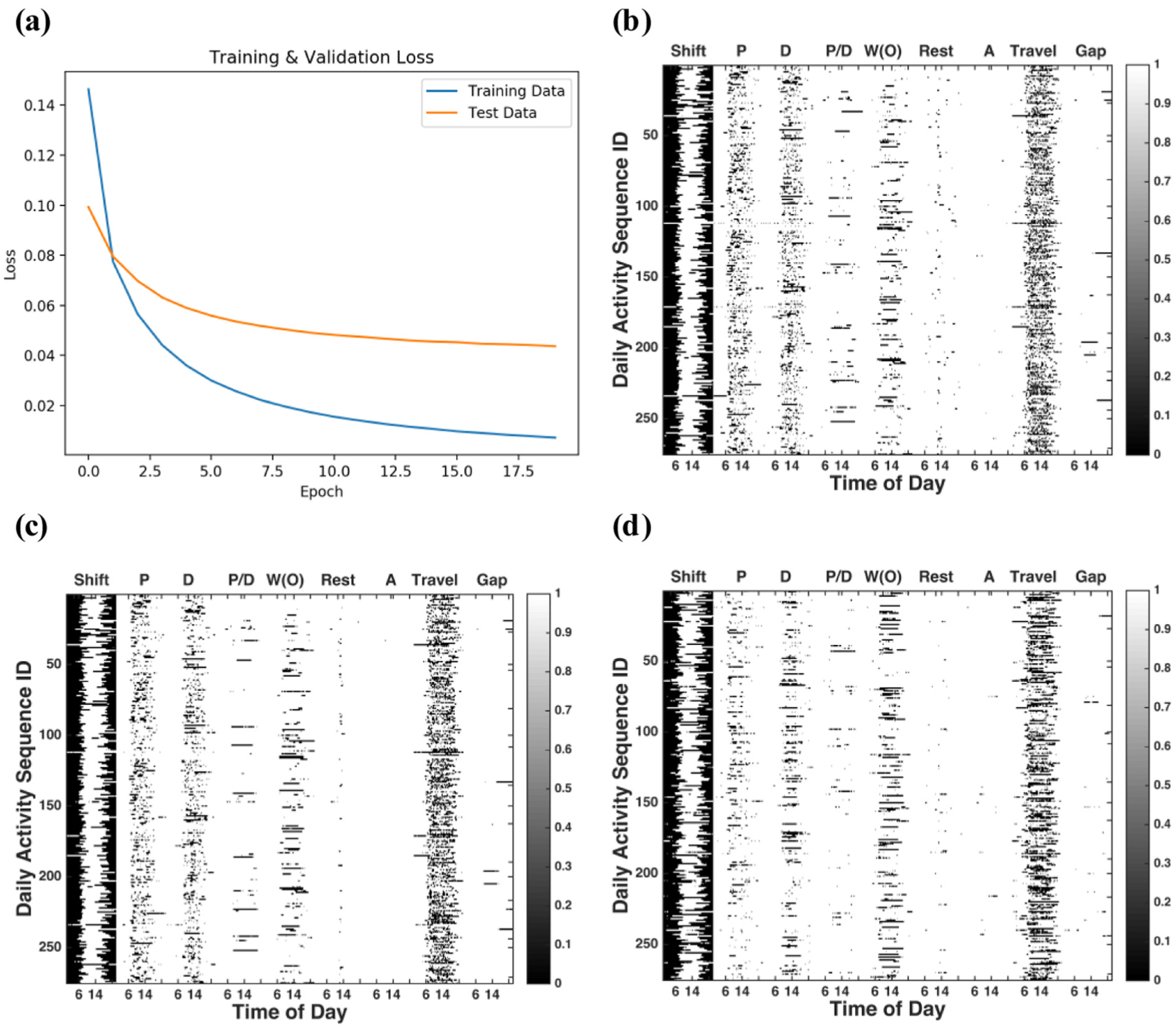
Autoencoder: (a) training and testing loss over epochs; (b) the test dataset; (c) the reconstruction with 25 encoding dimensions; (d) the simulated data with VAE.
This paper also experimented with implementing VAE to generate realistic-looking activity sequences. Kingma and Welling provide a reference on how VAE is implemented in Tensorflow ( 14 ). The major difference from autoencoder is that VAE learns the latent variable space instead of the original input and thus can generate outputs. Logistic PCA can be cast as a VAE with a latent dimension of one, as each Bernoulli distribution has only one parameter.
The best VAE model was formulated as follows. Encoder had two layers of LeakyRelu of dimensions 300 and 25; decoder had one layer of LeakyRelu and one layer of Sigmoid with dimensions of 300 and 2,592. The latent dimension was selected to be 8. Other settings follow from the autoencoder model described previously. Figure 4d presents one simulated activity matrix, based on the latent parameter space learned by the best VAE model. The error from the test dataset, 10.43%, was high, Nonetheless, it resembles Figure 4b, especially in capturing less major activities such as “Anomaly.” Further research is required to evaluate whether insights on freight behaviors derived based on the simulated activity sequences are the same as the real ones.
Validity of Applying PCA, Logistic PCA, Autoencoder and VAE
For PCA to apply, it is generally assumed that the input data follows a multivariate Gaussian distribution. When the input data is an activity matrix, as defined in Equation 2, it is non-Gaussian. Consequently, the derived principal components, that is, eigenbehaviors, are not strictly orthogonal, though, overlaps in the behaviors different principal components measure can exist. However, as commented by Jiang et al. PCA is still employed in a wide range of similar studies involving non-Gaussian data because orthogonality of principal components is not needed if the study purpose is not related to regression, or intended to reveal the probability distribution of input data ( 4 ). Logistic PCA only assumes each element in the input data to be a Bernoulli random variable. The binary nature of the activity matrix is more applicable to logistic PCA. However, logistic PCA requires estimating the natural parameters of Bernoulli distributions before computing principal components, which is a non-trivial task and usually only an approximated value is available. Autoencoder and VAE are built on feedforward networks, which do not have probabilistic assumptions, and thus remain valid for the task of reconstructing travel activity data.
Findings: Patterns of Truck Drivers’ Daily Activities
By employing the best PCA model to the dataset, the top three eigenbehaviors, which are eigenvectors computed by PCA, revealed interesting facts about truck drivers’ behaviors. In Figure 5, the color in each eigenbehavior represents the likelihood of one activity occurring across different times in a day: red at 0.1 denotes the highest probability of engaging in one activity; blue at −0.1 denotes the highest probability of the activity not happening; green at 0 denotes no inference.
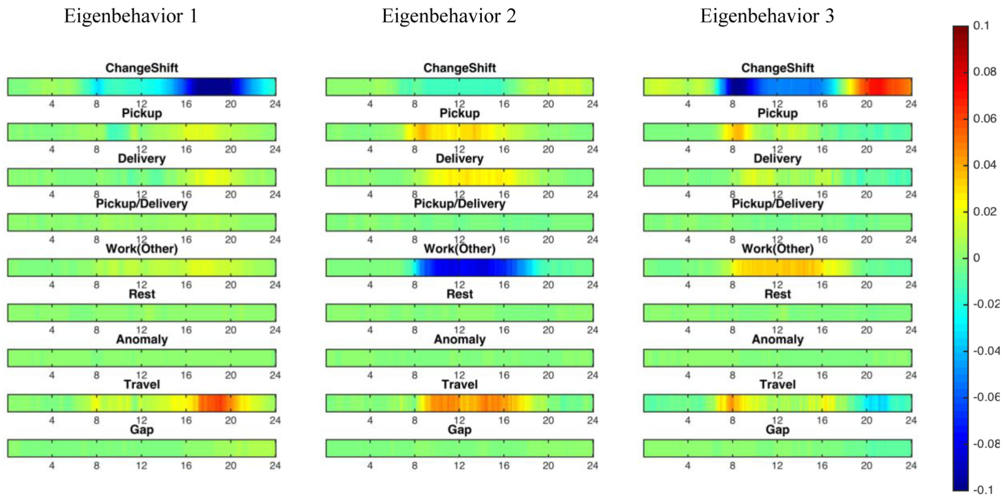
Top three activity patterns of urban truck drivers identified via PCA.
Eigenbehavior 1 revealed that the most distinguishing feature of a driver’s activity sequence was whether the driver was on shift from 4:00 to 8:00 p.m., and traveled extensively during this period. This may be because 4:00 to 8:00 p.m. is not a common work shift, so it captures the most variance in truck driver behaviors.
Eigenbehavior 2 explained the second largest behavior variance. It revealed a pattern in which drivers engage in “Pickup” and “Delivery” activities from 8:00 a.m. to 7:00 p.m., and were not likely to perform “Work (other)” during this period. As providing services is also categorized as “Work (other),” this pattern mainly describes the drivers who do not provide services but travel frequently during work hours to pick up and deliver goods. Delivery activity happened slightly after Pickup, but both had similar durations.
Eigenbehavior 3 described a pattern as follows: on shift from 7:00 a.m. to 4:00 p.m., traveled extensively around 8:00 a.m., performed the first “Pickup” around 8:00 a.m. and engaged in other work-related activities until going off shift. This might depict the daily routine of a road maintenance worker who picks up tools first and provides services afterwards.
Conclusion
This study explored different dimensionality reduction methods to reveal the activity patterns of truck drivers. Although PCA has been widely applied in uncovering patterns from passenger mobility ( 2 , 4 , 8 ), other dimensionality methods have not been developed in identifying activity patterns. As freight activity varies fundamentally from passenger activity, this paper set out to find a suitable method. Logistic PCA, autoencoder, and VAE techniques were investigated to reconstruct travel activity, to reveal the underlying behavior structure. In terms of reconstruction performance, all methods yielded less than 5% error. PCA gave the most truthful reconstruction, with an error of 0.99%, followed by autoencoder and logistic PCA. Nonetheless, autoencoder brought down the dimensions needed to 1% of the original dimensionality while sacrificing 0.5% in reconstruction error. When the dataset becomes too large for PCA to be applied efficiently, autoencoder is an ideal alternative. When assessing how interpretable the patterns discovered by each method were, PCA and logistic PCA were readily interpretable, whereas autoencoder was not. Finally, one critical advantage that autoencoder and VAE have is that they can easily incorporate the “space” dimension. PCA and logistic PCA take 2D matrices as input, whereas autoencoder and VAE can process multi-dimensional tensors. In studying freight behaviors, activity location has a direct impact on traffic modeling. Revealing patterns with time, location, and activity is an important aspect that autoencoder and VAE are able to address. In future work, identifying activity patterns with a location element will be explored with autoencoders.
Overall, PCA appeared to be most suitable for intuitively understanding the existing patterns in the dataset. Logistic PCA, as a variation of PCA, provided the flexibility to study a single activity such as “Anomaly” in the truck driver dataset used, which occurs much less frequently. VAE was most suitable for extrapolation, that is, synthesizing new realistic-looking datasets.
Dimensionality reduction is an important technique that reveals the underlying structure of data from vast amount of inputs. By imposing constraints on dimensionality, the most salient aspects of the input are preserved ( 7 ). The methods developed in this paper are not restricted to freight activity datasets, they could be generalized to any travel dataset for unsupervised pattern discovery. With dimensionality reduction, researchers are able to comprehend the “signature” of an individual’s mobility and even compare how similar one individual is to another based on this signature.
One acknowledged limitation in the Singapore case study was the sampling bias. A large portion of drivers came from the construction industry, so the patterns identified may not be representative of the population. As the survey dataset expands, the plan is to continue exploring activities.
Footnotes
Acknowledgements
This research was supported by the Singapore Ministry of National Development and the National Research Foundation under the Land and Liveability National Innovation Challenge (Award no. L2NICTDF1-2016-1). We thank the Urban Redevelopment Authority of Singapore, JTC Corporation, and Land Transport Authority of Singapore for their support.
Author Contributions
The authors confirm contribution to the paper as follows: study conception and design: Lu, Cheah; data collection: Lu, Zhao, Cheah; analysis and interpretation of results: Lu, Zhao, Cheah; draft manuscript preparation: Lu, Zhao, Cheah. All authors reviewed the results and approved the final version of the manuscript.
The Standing Committee on Freight Transportation Planning and Logistics (AT015) peer-reviewed this paper (18-03813).
The opinions, findings, and conclusions or recommendations expressed in this material are those of the authors only.