Sage Journals: Discover world-class research

Abstract

This paper proposes a method of assigning trips to automated taxis (ATs) and designing the routes of those vehicles in an urban road network, and also considering the traffic congestion caused by this dynamic responsive service. The system is envisioned to provide a seamless door-to-door service within a city area for all passenger origins and destinations. An integer programming model is proposed to define the routing of the vehicles according to a profit maximization function, depending on the dynamic travel times, which varies with the ATs’ flow. This will be especially important when the number of automated vehicles (AVs) circulating on the roads is high enough that their routing will cause delays. This system should be able to serve not only the reserved travel requests, but also some real-time requests. A rolling horizon scheme is used to divide one day into several periods in which both the real-time and the booked demand will be considered together. The model was applied to the real size case study city of Delft, the Netherlands. The results allow assessing of the impact of the ATs movements on traffic congestion and the profitability of the system. From this case-study, it is possible to conclude that taking into account the effect of the vehicle flows on travel time leads to changes in the system profit, the satisfied percentage and the driving distance of the vehicles, which highlights the importance of this type of model in the assessment of the operational effects of ATs in the future.

In recent years, technology development has accelerated the future roll-out of vehicle automation. This technology is expected to have a beneficial impact on travel efficiency, especially on interurban roads. Studies have mostly used micro-simulation tools or mathematical models to estimate the changes in road capacity and congestion under different levels of vehicle automation and cooperation (1 –3).

Regarding the use of automated vehicles (AVs) as transit systems, there are currently several projects which are testing the implementation automated pods or buses in pilot experiments. One of the most relevant examples being the CityMobil2 project ( 4 ) in which different field experiments are being run in several European cities. In 2015 the province of Gelderland in the Netherlands started developing a project named WEpods with two self-driving vehicles, which are being tested within the Wageningen University campus, and between the campus and Ede-Wageningen train station ( 5 ).

Several approaches have been proposed to test the effect of transit automation on mobility, especially looking at the combination between traditional taxis and shared use taxi fleets. The automated taxis (ATs) may provide a new type of door-to-door service competing with traditional taxis or even public transport because these new systems would be able to avoid extra manpower costs and make the ATs service cheaper. Two methods are widely used to test the impact of AVs as public transport, agent-based simulation and mathematical optimization. Martinez et al. used agent-based simulation to build a model to test the introduction of 100% autonomous fleets of taxis to satisfy transport demand in a city ( 6 ). Spieser et al. used an analytical mathematical formulation to estimate the number of shared AVs to replace all modes of personal transportation in the case-study city of Singapore ( 7 ). Liang et al. proposed two integer programming models to optimize the service area of ATs for the last mile of train trips. Applying the methods to the real case-study city of Delft, the Netherlands, they concluded that fleet size influences the profitability of the taxi system ( 8 ). Despite these models and their application, they all seem to be limited in having taken into account the effect that the taxis themselves can have on the traffic flow, and hence the delays in the network.

A recent study addressed the traffic assignment of privately owned AVs from the user optimum perspective with the objective of minimizing each family’s own transport costs ( 9 ). An equilibrium convergence was proposed in which households with similar trips should have similar transport costs. Since traffic assignment is a nonlinear problem, this was tackled by an iterative process in which travel times do not change during each assignment of vehicles to trips and to the network. Another study also considered the traffic congestion when studying the routing problem of a large number of shared AVs, in which the traffic flow is modeled through link-transmission model ( 10 ). Then the model is applied to a small network as the considerable computation time means this formulation is not ready to solve the AVs’ dynamic routing problems on a real size network.

In this paper, a model is proposed to address the problem of assigning the vehicles to clients and to paths on the urban road network. The model should consider dynamic travel times, which vary with the flow of the ATs. Moreover, it does not only serve reserved requests, but also some real-time requests. A rolling horizon scheme is proposed in which an optimization problem is solved over several horizons with updated demand. This approach advantage is two-fold: it helps reduce the problem size and it allows for adaption of the supply to the real-time demand.

Rolling horizon is a standard solution methodology for the dynamic vehicle routing problem ( 11 ). It is achieved by repeatedly solving a static problem over the events that have occurred from the current time $t$ , to $t + L$ , where $L$ is the length of a horizon. Double-horizon based heuristics were proposed by Mitrović-Minić et al., incorporating both the long-term and short-term horizons ( 12 ). Yang et al. presented a rolling horizon scheme for truck fleet assignment and scheduling, when dealing with the real-time information ( 13 ). Luo and Schonfeld compared the rolling horizon strategy with the immediate strategy when inserting requests implemented in dial-a-ride problem heuristics. They concluded from their computation results that when satisfying all of the demand, the rolling horizon strategy reduced the vehicles by up to 10%, compared with the immediate strategy. This is because the rolling horizon strategy benefits from the advance information available ( 14 ).

The paper is organized as follows. Firstly, it introduces the mathematical model for assigning the passengers’ requests to ATs and searching the optimal vehicle routing solutions. Secondly, the rolling horizon scheme is described to deal with the reserved and real-time requests. Then the application to the case-study city of Delft is presented, which is followed by the results of comparing the running of the model with and without congestion. The paper ends with the main conclusions that can be taken from the model application.

Integer Programming Model

This section describes a linear programming model for which the objective is to determine the optimal vehicle routing of the ATs system. A private taxi service can serve any pair of nodes within the city road network in which it is assumed that there is no background traffic flow, meaning the flow is generated only by the ATs themselves. Clients use an online app to book ATs providing travel information that includes the origin, the destination and the desired departure time. The model works on the assumption that the taxi company can achieve total control of the system by being free to accept or reject requests according to a profit maximization objective. It is assumed that the system accepts only individual trips for each vehicle. The model sets, data, parameters and mathematical formulation are shown below.

Sets

$N = {1, \dots, i, \dots N}$ : set of the nodes in the network, in which $N$ is the total number of nodes.

$T = {0, \dots, t, \dots, T}$ : set of time instants in the service period, in which $T$ is the total number of time steps in the operation time.

$T^{'} = {- T^{b}, \dots 0, \dots, t, \dots, T, \dots, T + T^{b}}$ : set of time instants in the operation time, including the service period ${0 \dots T}$ and the buffer period ${- T^{b} \dots 0}$ and ${T \dots T + T^{b}}$ , in which $T^{b}$ is the number of time steps in the buffer period.

$E = {1, \dots, e, \dots, E}$ : set of trips, in which $E$ is the total number of all the trips in the operation time.

$V = {1, \dots, v, \dots, V}$ : set of vehicles, in which $V$ is the total number of taxis in the system.

$K = {0, \dots, k, \dots, K}$ : set of break-points when calculating the travel time based on the traffic flow, in which $K$ is the total number of the break-points.

$A = {\dots, (i, j), \dots}$ : set of connected links of the road network, in which vehicles move, $i, j \in N$ , i ≠ j $i \neq j$

$B = {\dots, (i_{t_{1}}, j_{t_{2}}), \dots}$ : set of links in the time-space network, $\forall (i, j) \in A, \forall t_{1}, t_{2} \in T^{'}, t_{1} < t_{2}, δ_{i j}^{m i n} \leq t_{2} - t_{1} \leq δ_{i j}^{m a x}$

Data

$a^{e}$ : desired departure time for the $e$ ^th trip, $e \in E$

$b^{e}$ : latest arrival time for the $e$ ^th trip, $e \in E$

$c^{e}$ : earliest departure time for the $e$ ^th trip, $e \in E$

$w a i t^{e}$ : maximum waiting time for departing on the $e$ ^th trip, $e \in E$

$o r i^{e}$ : the origin node for the $e$ ^th trip, $e \in E$

$d e s^{e}$ : the destination node for the $e$ th trip, $e \in E$

$δ_{i j}^{m a x}$ : maximum travel time from node $i$ to node $j$ in time steps, $\forall (i, j) \in A$

$δ_{i j}^{m i n}$ : minimum travel time from node $i$ to node $j$ in time steps, $\forall (i, j) \in A$

$δ_{i j}^{k}$ : travel time from node $i$ to node $j$ in time steps at break-point $k$ , $\forall (i, j) \in A, k \in K$

$d_{i j}$ : length of the link $(i, j)$ in kilometers, $\forall (i, j) \in A$

$O p t_{i j}$ : shortest travel time from node $i$ to node $j$ in free-flow conditions, $\forall i, j \in N$

$C a p_{i j} :$ capacity of each link $(i, j)$ which is the number of vehicles that can go through the link at the highest travel time, $\forall (i, j) \in A$

Parameters

$P r$ : price rate of a taxi, € / time step

$C_{f u e l}$ : fuel cost, €/ km

$C_{p}$ : parking cost, € / time step

$C_{d}$ : vehicle depreciation cost, € / day

$ρ$ : penalty cost if a trip is rejected by the system, € / trip

$C_{w}$ : penalty for passengers’ waiting, € / time step

$C_{d e l}$ : penalty for delivery delay, where the delay is defined as the real travel time minus the shortest travel time for a request, € / time step

$μ$ µ: expansion coefficient, represents the number of taxis with the same characteristics in the population

Decision Variables

$x_{i_{t_{1},} j_{t_{2}}}^{v}$ : binary variable equal to 1 if vehicle $v$ drives from $i$ to $j$ from time instant $t_{1}$ to $t_{2}$ , $\forall (i_{t_{1}}, j_{t_{2}}) \in B, \forall v \in V$

$y_{i_{t}}^{v}$ : binary variable equal to 1 if vehicle $v$ parks at $i$ from time instant $t$ to $t + 1$ , $\forall i \in N$ , $\forall v \in V$ , $\forall t \in T^{'}, t < T$

$S_{i j}^{e v}$ : binary variable equal to 1 if trip $e$ from node $i = o r i^{e}$ to node $j = d e s^{e}$ is done using vehicle $v$ , $\forall e \in E$ , $\forall v \in V$

$P_{i j}^{e v t}$ : binary variable equal to 1 if trip $e$ from node $i = o r i^{e}$ to node $j = d e s^{e}$ done by vehicle $v$ starts at time instant $t$ , $\forall e \in E$ , $\forall v \in V$ , $\forall t \in T, c^{e} \leq t \leq a^{e} + w a i t^{e}$

$A_{i j}^{e v t}$ : binary variable equal to 1 if trip $e$ from node $i = o r i^{e}$ to node $j = d e s^{e}$ done by vehicle $v$ ends at time instant $t$ , $\forall e \in E$ , $\forall v \in V$ , $\forall t \in T^{'}, c^{e} + O p t_{i j} \leq t \leq b^{e}$

$ϕ_{i j}^{e v}$ : integer variable of the difference between the desired pick-up time and real pick-up time of trip $e$ from node $i = o r i^{e}$ to node $j = d e s^{e}$ done by vehicle $v$ , $\forall e \in E$ , $\forall v \in V$

$L o a d_{t}^{v}$ : binary variable equal to 1 if vehicle $v$ is transporting an individual passenger from time instant $t$ to $t + 1$ , $\forall v \in V$ , $\forall t \in T^{'}, t < T$

$F_{i j}^{t}$ : integer variable of the vehicle flow on link $(i j)$ starting from time instant $t$ , $\forall (i, j) \in A$ , $\forall t \in T^{'}, t < T^{'}$

$λ_{i j}^{t, k}$ : binary variable equal to 1 if travel time on link $(i j)$ starting from $t$ is at break-point $k$ , $\forall (i, j) \in A$ , $\forall t \in T^{'}, t < T^{'}$ , $\forall k \in K$

$δ_{i j}^{t}$ : integer variable of travel time when travelling on link $(i j)$ starting from time instant $t$ in time steps, $\forall (i, j) \in A$ , $\forall t \in T^{'}, t < T^{'}$

Objective Function

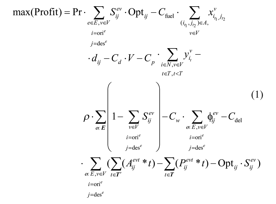
\begin{array}{l} \max (P r o f i t) = P r \cdot \sum_{\begin{matrix} e \in E, v \in V \\ i = o r i^{e} \\ j = d e s^{e} \end{matrix}} S_{i j}^{e v} \cdot O p t_{i j} - C_{f u e l} \cdot \sum_{\begin{matrix} (i_{t_{1}}, j_{t_{2}}) \in A, \\ v \in V \end{matrix}} x_{i_{t_{1},} j_{t_{2}}}^{v} \\ \cdot d_{i j} - C_{d} \cdot V - C_{p} \cdot \sum_{\begin{matrix} i \in N, v \in V \\ t \in T, t < T \end{matrix}} y_{i_{t}}^{v} - \\ ρ \cdot \sum_{e ϵ E} (1 - \sum_{\begin{matrix} v \in V \\ i = o r i^{e} \\ j = d e s^{e} \end{matrix}} S_{i j}^{e v}) - C_{w} \cdot \sum_{\begin{matrix} e ϵ E, v \in V \\ i = o r i^{e} \\ j = d e s^{e} \end{matrix}} ϕ_{i j}^{e v} - C_{d e l} \\ \cdot \sum_{\begin{matrix} e ϵ E, v \in V \\ i = o r i^{e} \\ j = d e s^{e} \end{matrix}} (\sum_{t \in T^{'}} (A_{i j}^{e v t} * t) - \sum_{t \in T} (P_{i j}^{e v t} * t) - O p t_{i j} \cdot S_{i j}^{e v}) \end{array}

The objective function is considered from the perspective of both the ATs company and the passenger. For the ATs company, it aims to maximize the total profit which includes the total revenue from the customers, the vehicle fuel costs, the vehicle depreciation costs and the parking costs. The revenue is only charged for the shortest travel time of each request to avoid extra detours to charge more to the client. Regarding the passengers, when a request is rejected, passengers are assumed to use public transport as an alternative to finish their trip and the ATs system should pay a fixed charge for the users as a penalty. Late arrival and delivery delay are also penalized to consider the level of service offered to the clients.

Subject to the Following Constraints

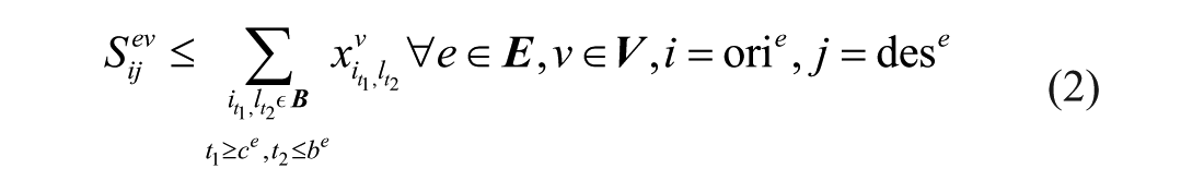
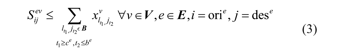
The constraints given in Equation 2 describe that trip $e$ from node $i$ to node $j$ can only be satisfied by vehicle $v$ if that vehicle has passed through node $i$ between the earliest departure time $c^{e}$ and the latest arrival time $b^{e}$ :

S_{i j}^{e v} \leq \sum_{\begin{matrix} i_{t_{1},} l_{t_{2}} ϵ B \\ t_{1} \geq c^{e}, t_{2} \leq b^{e} \end{matrix}} x_{i_{t_{1},} l_{t_{2}}}^{v} \forall e \in E, v \in V, i = o r i^{e}, j = d e s^{e}

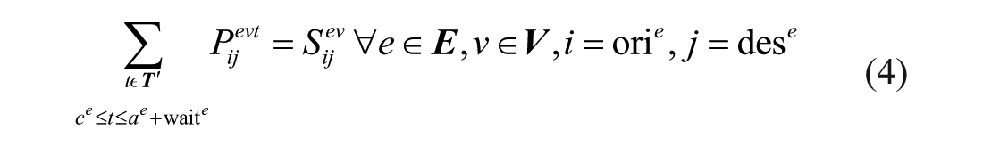
The constraints given in Equation 3 describe that trip $e$ from node $i$ to node $j$ can only be satisfied by vehicle $v$ if that vehicle has passed through node $j$ at time instant $a^{e} + δ_{i j}$ :

S_{i j}^{e v} \leq \sum_{\begin{matrix} l_{t_{1},} j_{t_{2}} ϵ B \\ t_{1} \geq c^{e}, t_{2} \leq b^{e} \end{matrix}} x_{l_{t_{1},} j_{t_{2}}}^{v} \forall v \in V, e \in E, i = o r i^{e}, j = d e s^{e}

The constraints given in Equation 4 assure that a satisfied trip must have only one departure time or this trip is not satisfied at all:

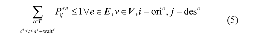
\sum_{\begin{matrix} t ϵ T^{'} \\ c^{e} \leq t \leq a^{e} + w a i t^{e} \end{matrix}} P_{i j}^{e v t} = S_{i j}^{e v} \forall e \in E, v \in V, i = o r i^{e}, j = d e s^{e}

The constraints given in Equation 5 guarantee that one trip can only have one departure time when it is served or this trip is not satisfied by any vehicle:

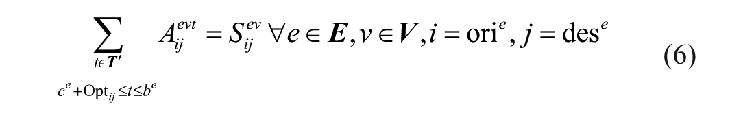
\sum_{\begin{matrix} t \in T \\ c^{e} \leq t \leq a^{e} + w a i t^{e} \end{matrix}} P_{i j}^{e v t} \leq 1 \forall e \in E, v \in V, i = o r i^{e}, j = d e s^{e}

The constraints given in Equation 6 assure that a satisfied trip must have only one arrival time or this trip is not satisfied at all:

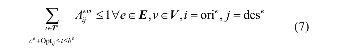
\sum_{\begin{matrix} t ϵ T^{'} \\ c^{e} + O p t_{i j} \leq t \leq b^{e} \end{matrix}} A_{i j}^{e v t} = S_{i j}^{e v} \forall e \in E, v \in V, i = o r i^{e}, j = d e s^{e}

The constraints given in Equation 7 guarantee that one trip can only have one arrival time when it is served or this trip is not satisfied by any vehicle:

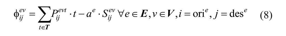
\sum_{\begin{matrix} t \in T^{'} \\ c^{e} + O p t_{i j} \leq t \leq b^{e} \end{matrix}} A_{i j}^{e v t} \leq 1 \forall e \in E, v \in V, i = o r i^{e}, j = d e s^{e}

The constraints given in Equation 8 compute the difference between the desired departure time and the real departure time, which is the passengers’ waiting time:

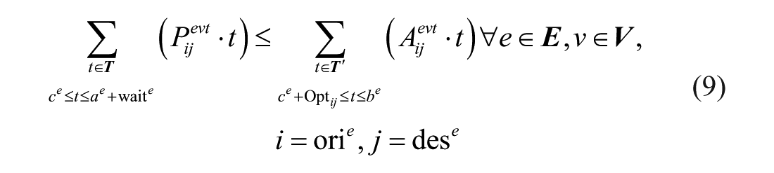
ϕ_{i j}^{e v} = \sum_{t \in T} P_{i j}^{e v t} \cdot t - a^{e} \cdot S_{i j}^{e v} \forall e \in E, v \in V, i = o r i^{e}, j = d e s^{e}

The constraints given in Equation 9 impose that the departure time instant of a satisfied trip must happen before the arrival time instant:

\begin{array}{l} \sum_{\begin{matrix} t \in T \\ c^{e} \leq t \leq a^{e} + w a i t^{e} \end{matrix}} (P_{i j}^{e v t} \cdot t) \leq \sum_{\begin{matrix} t \in T^{'} \\ c^{e} + O p t_{i j} \leq t \leq b^{e} \end{matrix}} (A_{i j}^{e v t} \cdot t) \forall e \in E, v \in V, \\ i = o r i^{e}, j = d e s^{e} \end{array}

The constraints given in Equation 10 ensure that a trip can only be served by one vehicle:

\sum_{v \in V} S_{i j}^{e v} \leq 1 \forall e \in E, i = o r i^{e}, j = d e s^{e}

The constraints given in Equation 11 impose that for a specific time step $t$ to $t + 1$ each one of the ATs should only park at one node or not park at all:

\sum_{i \in N} y_{i_{t}}^{v} \leq 1 \forall v \in V, t \in T^{'}, t < T^{'}

The constraints given in Equation 12 guarantee that one trip with a specific origin and departure time can only have one destination and one arrival time:

\sum_{i_{t_{1},} j_{t_{2}} \in B} x_{i_{t_{1},} j_{t_{2}}}^{v} \leq 1 \forall i \in N, v \in V, t_{1} \in T^{'}

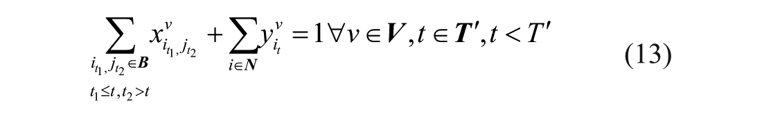
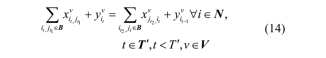
The constraints given in Equation 13 ensure that each vehicle can only have one status at time instant $t$ : either going to the next destination or parking at that place:

\sum_{\begin{matrix} i_{t_{1},} j_{t_{2}} \in B \\ t_{1} \leq t, t_{2} > t \end{matrix}} x_{i_{t_{1},} j_{t_{2}}}^{v} + \sum_{i \in N} y_{i_{t}}^{v} = 1 \forall v \in V, t \in T^{'}, t < T^{'}

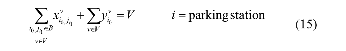
The constraints given in Equation 14 are flow conservation constraint which make sure that the number of taxis leaving from node $i$ and parking there from time instant $t$ is equal to the number of vehicles arriving at node $i$ and parking at the same place until $t$ :

\begin{array}{l} \sum_{i_{t,} j_{t_{1}} \in B} x_{i_{t,} j_{t_{1}}}^{v} + y_{i_{t}}^{v} = \sum_{i_{t_{2},} j_{t} \in B} x_{j_{t_{2},} i_{t}}^{v} + y_{i_{t - 1}}^{v} \forall i \in N, \\ t \in T^{'}, t < T^{'}, v \in V \end{array}

The constraints given in Equation 15 describe the initial status of the ATs fleet. At the beginning of the operation period, all vehicles are stocked at the central parking station:

\sum_{\begin{matrix} i_{0,} j_{t_{1}} \in B \\ v \in V \end{matrix}} x_{i_{0,} j_{t_{1}}}^{v} + \sum_{v \in V} y_{i_{0}}^{v} = V i = p a r k i n g s t a t i o n

The constraints given in Equation 16 compute the flow of vehicles in each road link $(i, j)$ from time instant $t_{1}$ :

F_{i j}^{t_{1}} = (\sum_{v \in V} x_{i_{t_{1},} j_{t_{2}}}^{v}) \cdot μ \forall (i_{t_{1}}, j_{t_{2}}) \in B

The constraints given in Equation 17 limit the flow to the capacity of each link:

F_{i j}^{t} \leq Q_{i j} \forall (i, j) \in A, \forall t \in T^{'}, t < T^{'}

The constraints given in Equations 18 and 19 impose a break-point $k$ to describe the congestion level of each link:

F_{i j}^{t} = \sum_{k \in K} λ_{i j}^{t, k} \cdot k \cdot μ \forall (i, j) \in A, \forall t \in T^{'}, t < T^{'}

\sum_{k \in K} λ_{i j}^{t, k} = 1 \forall (i, j) \in A, \forall t \in T^{'}, t < T^{'}

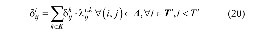
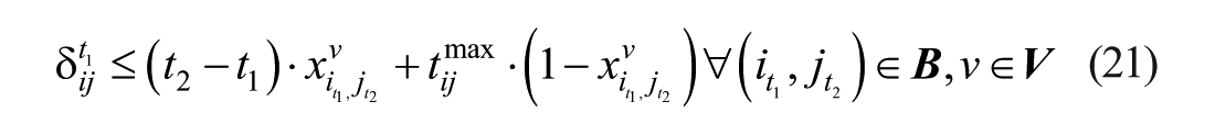
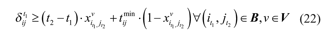
The constraints given in Equation 20 define the travel time on road link $(i, j)$ from time instant $t$ based on the break-point $k$ :

δ_{i j}^{t} = \sum_{k \in K} δ_{i j}^{k} \cdot λ_{i j}^{t, k} \forall (i, j) \in A, \forall t \in T^{'}, t < T^{'}

The constraints given in Equations 21 and 22 impose that the travel time is not greater than the maximum travel time or smaller than the minimum travel time. Meanwhile, they also guarantee that when vehicle $v$ is travelling on link ( $i_{t_{1},} j_{t_{2}})$ , the travel time must be $δ_{i j}^{t_{1}}$ :

δ_{i j}^{t_{1}} \leq (t_{2} - t_{1}) \cdot x_{i_{t_{1},} j_{t_{2}}}^{v} + t_{i j}^{m a x} \cdot (1 - x_{i_{t_{1},} j_{t_{2}}}^{v}) \forall (i_{t_{1}}, j_{t_{2}}) \in B, v \in V

δ_{i j}^{t_{1}} \geq (t_{2} - t_{1}) \cdot x_{i_{t_{1},} j_{t_{2}}}^{v} + t_{i j}^{m i n} \cdot (1 - x_{i_{t_{1},} j_{t_{2}}}^{v}) \forall (i_{t_{1}}, j_{t_{2}}) \in B, v \in V

The constraints given in Equation 23 guarantees link consistency. It is assumed that vehicles entering on a link $(i, j)$ later from node $i$ should not leave earlier from node $j$ , which means the ATs do not pass one another. These constraints were established by Kaufman et al. ( 15 ):

t_{1} + δ_{i j}^{t_{1}} \leq t_{2} + δ_{i j}^{t_{2}} \forall (i, j) \in A, t_{1}, t_{2} \in T^{'}, t_{1}, t_{2} < T^{'}, t_{1} < t_{2}

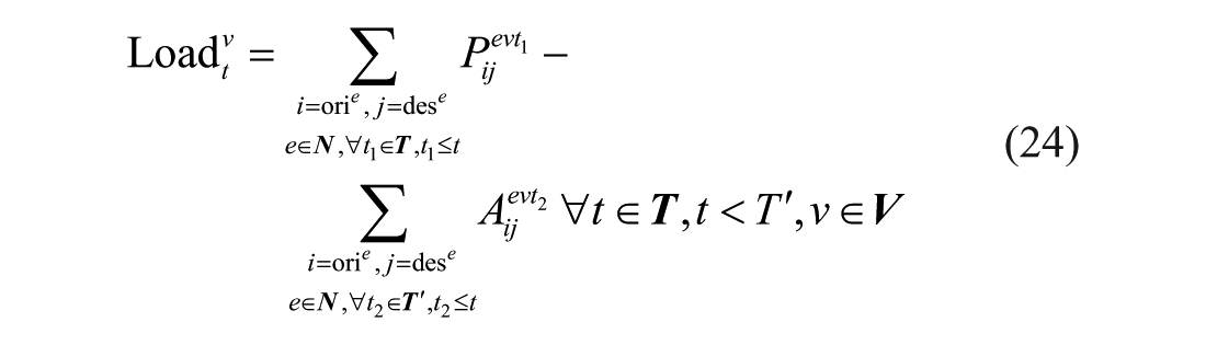
The constraints given in Equation 24 compute the number of passengers loaded on each vehicle during time step $t$ to $t + 1$ :

\begin{array}{l} L o a d_{t}^{v} = \sum_{\begin{matrix} i = o r i^{e}, j = d e s^{e} \\ e \in N, \forall t_{1} \in T, t_{1} \leq t \end{matrix}} P_{i j}^{e v t_{1}} - \\ \sum_{\begin{matrix} i = o r i^{e}, j = d e s^{e} \\ e \in N, \forall t_{2} \in T^{'}, t_{2} \leq t \end{matrix}} A_{i j}^{e v t_{2}} \forall t \in T, t < T^{'}, v \in V \end{array}

The constraints given in Equation 25 enforce that only one passenger can be in each vehicle. In addition, when the vehicle is transporting passengers, it should not park at any node of the road network:

L o a d_{t}^{v} + \sum_{i \in N} y_{i_{t}}^{v} \leq 1 \forall t \in T, t < T^{'}, v \in V

Rolling Horizon

The mathematical model described in the previous section entails knowing all the demand before the optimization. This means all taxi system users should reserve this transport service and provide all the travel information including the origin, the destination, and the departure time beforehand. Therefore, it would be impossible to change the movement of the ATs and serve real-time demand. Using a rolling horizon scheme, it is possible to consider those requests and at the same time reduce the complexity of the model that was proposed above.

Rolling Horizon Scheme

A rolling horizon scheme is used to divide one day into several horizons in which both the real-time and the pre-booked demand are considered. Model constraints given in Equations 1 –25 are run for every horizon with updated demand from the previous. The horizon rolls forward with a specific rolling length and arrives at the next horizon with updated ATs requests. In this section, $H = {1, \dots, h, \dots H}$ is the set of horizons in a day, in which $H$ is the total number of horizons. $t_{r}$ is the time length for rolling, and $t_{h}$ is the time length of a horizon, $t_{r} < t_{h}$ .

The rolling horizon scheme is shown in Figure 1. For horizon 1, the system collects the reserved requests which have the desired departure time within the time horizon 0 to $t_{h}$ as input I and optimizes the ATs movements using these requests. After obtaining the optimal results as output I, the ATs system only executes the routing results for each vehicle from 0 to $t_{r}$ (output II) and rolls forward to the next horizon. For the second horizon, two types of demand are both entered into the system. In addition to the reserved requests from $t_{r}$ to $t_{r} + t_{h}$ (input I), the ATs company also receives real-time demand to be served as soon as possible from 0 to $T_{r}$ as input II (these cannot be served at the rolling interval in which they were generated due to the vehicles’ routes already being optimized). The optimization process for horizon 2 will be performed just before the time instant $T_{r}$ , and all the ATs only perform the optimal results for $T_{r}$ to $t_{r} + t_{r}$ (output II). Similarly, when it rolls to horizon $h$ , the system input will be the reserved requests for $(h - 1) \cdot t_{r}$ to $(h - 1) \cdot t_{r} + t_{h}$ and the real-time requests for $(h - 2) \cdot t_{r}$ to $(h - 1) \cdot t_{r}$ . Then the system will only implement the routing results for $(h - 1) \cdot t_{r}$ to $h \cdot t_{r}$ as output II out of all the potential results for $(h - 1) \cdot t_{r}$ to $(h - 1) \cdot t_{r} + t_{h} + t_{b}$ which is the output I of horizon $h$ .

Figure 1.

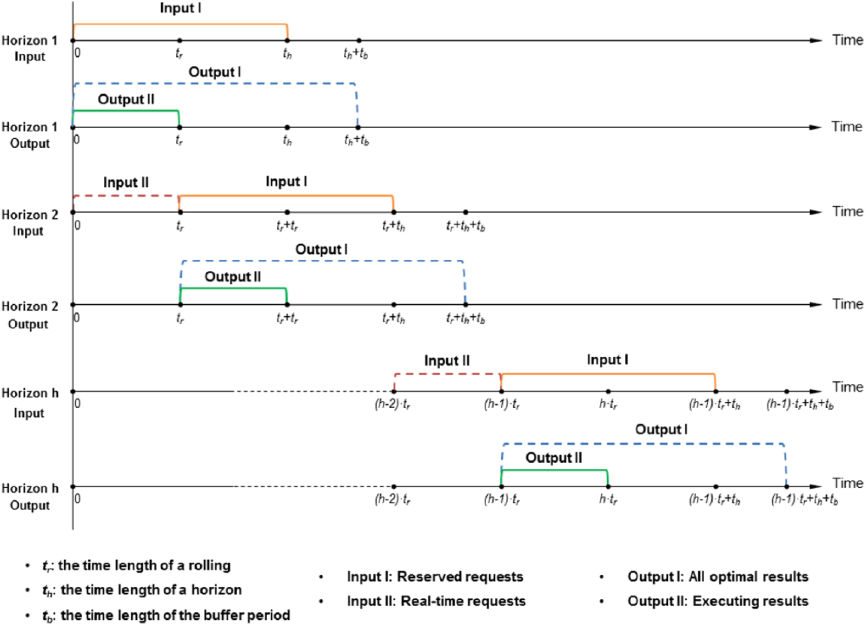
Rolling horizon scheme.

The rolling length and the horizon length can be explained from a practical perspective. This rolling horizon scheme is able to optimize the ATs’ routing time after time with real-time information. The horizon length determines how far the system will include the pre-known information: the reserved taxi service requests. The rolling length indicates how often the system will input the new requests, update the optimal results and execute the routing plan. The rolling length is set shorter than the horizon length because the system can plan for the future requests and update once new requests enter. If the horizon is as short as a rolling length, the system cannot relocate for the next horizon trip, which may decrease the system efficiency. If the rolling is as long as the horizon, the real-time request clients may wait for a whole horizon to be calculated for optimization.

Demand Initialization

Different time components for reserved and real-time requests are set to initialize the system demand. The reserved requests arrive in advance before the horizon start time. No waiting time is allowed to provide a better service for these clients. This means the system should serve them as they require. As a result, the desired departure time is also the earliest departure time for this kind of demand. For the real-time requests, the time they make requests is the desired departure time. Therefore, this model allows some waiting time for each request to be served by ATs as these requests are only analyzed in the next horizon. The earliest departure time is the start time of the current horizon. In this model, the maximum waiting time is set equal to the time length for rolling.

For horizon $h$ , the desired departure time $a^{e, h}$ for each request should be transformed from an absolute time to a relative time: $a^{e h} = a^{e} - (h - 1) * t_{r}$ . The earliest departure time for reserved requests in horizon $h$ is: $c^{e h} = a^{e, h}$ . The earliest departure time for real-time requests in horizon $h$ is: $c^{e h} = 0$ . The latest arrival time for reserved requests in horizon $h$ is: $b^{e h} = a^{e h} + O p t_{i j} \cdot δ$ . The latest arrival time for real-time requests in horizon $h$ is: $b^{e h} = w a i t^{e} + O p t_{i j} \cdot δ$ , where $δ$ is the scale factor between the maximum travel time and the shortest travel time.

Continuity

There are three types of satisfied trips in each optimization horizon which can be handled in different ways in the rolling horizon scheme (Figure 2). If the optimal departure time and the arrival time for each request are both within the executing period (from $(h - 1) * t_{r}$ to $h * t_{r}$ ), the system will fully execute the routing results for that request (trip type 1). If the departure and arrival time are both after the end of the executing period $t_{r}$ , the system will leave it in the demand pool and perform the optimization later in the next horizon (trip type 2). If the departure time is before $t_{r}$ and the arrival time is afterward (trip type 3), then the system will execute the routing results from the departure time until $t_{r}$ . Based on the optimal solution, the system will know which vehicle satisfies this request and the location of it at time instant $t_{r}$ . This location will be the new origin of that request and this time is the new departure time in the next horizon. In some cases, at time instant $t_{r}$ the vehicle $v$ is in the middle of a road link. The cut-off time for this request will be the one closest to $t_{r}$ after $t_{r}$ , and the new origin of it will be the location of vehicle $v$ at that time instant.

Figure 2.

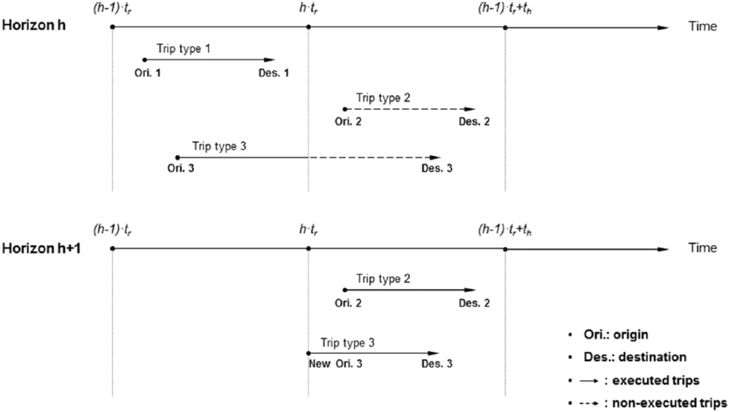
Trips between horizons.

When obtaining the optimal results from the previous horizon, some new notations are used to save the system status information, and set them as a starting point for the next horizon:

$l o c^{v h}$ : the location of vehicle $v$ at or most close to the beginning of the current horizon, $\forall v \in V, h \in H$

$e t^{v h}$ : the first available time when vehicle $v$ finishes its trip starting from the last horizon, $\forall v \in V, h \in H$

$v s^{e h}$ : which vehicle satisfies trip $e$ in the previous horizon, $\forall e \in E, h \in H$

$v o_{i_{t}}^{v h}$ : equal to 1 if vehicle $v$ is occupied by an unfinished trip from time instant $t$ to $t + 1$ from the previous horizon, $\forall v \in V, t \in T^{'}, t < T^{'}, i = l o c^{v}, h \in H$

$v o_l a s t_{i_{t}}^{v h}$ : equal to 1 if vehicle $v$ is occupied by an unfinished trip from time instant $t$ to $t + 1$ from the previous horizon, and will end this trip at time instant $t + 1$ , $\forall v \in V, t \in T^{'}, t < T^{'}, i = l o c^{v h}, h \in H$

The equations below are used to save the vehicle status information from the previous horizon:

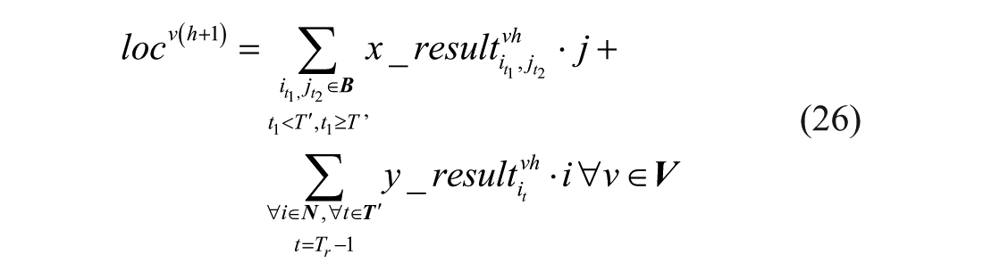
\begin{array}{l} l o c^{v (h + 1)} = \sum_{\begin{matrix} i_{t_{1},} j_{t_{2}} \in B \\ t_{1} < T^{'}, t_{1} \geq T ’ \end{matrix}} x_r e s u l t_{i_{t_{1}}, j_{t_{2}}}^{v h} \cdot j + \\ \sum_{\begin{matrix} \forall i \in N, \forall t \in T^{'} \\ t = T_{r} - 1 \end{matrix}} y_r e s u l t_{i_{t}}^{v h} \cdot i \forall v \in V \end{array}

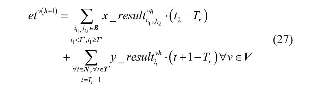
Equation (26) computes the final location of vehicle $v$ at the last time instant of the execute period $T_{r}$ , where $x_r e s u l t_{i_{t_{1}}, j_{t_{2}}}^{v h}$ is the value of decision variable $x_{i_{t_{1}}, j_{t_{2}}}^{v}$ from horizon $h - 1$ , and $y_r e s u l t_{i_{t}}^{v h}$ is the value of decision variable $y_{i_{t}}^{v}$ from horizon $h - 1$ . If this vehicle is on an unfinished trip, then the location will be the destination of that trip.

\begin{array}{l} e t^{v (h + 1)} = \sum_{\begin{matrix} i_{t_{1},} j_{t_{2}} \in B \\ t_{1} < T^{'}, t_{1} \geq T^{'} \end{matrix}} x_r e s u l t_{i_{t_{1}}, j_{t_{2}}}^{v h} \cdot (t_{2} - T_{r}) \\ + \sum_{\begin{matrix} \forall i \in N, \forall t \in T^{'} \\ t = T_{r} - 1 \end{matrix}} y_r e s u l t_{i_{t}}^{v h} \cdot (t + 1 - T_{r}) \forall v \in V \end{array}

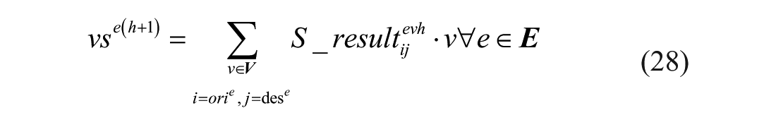
Equation (27) is equal to 0 if vehicle $v$ is free at the last time instant of the execute period $T_{r}$ . If it is not, it is the first available time when vehicle $v$ finishes its trip starting from the last horizon.

v s^{e (h + 1)} = \sum_{\begin{matrix} v \in V \\ i = o r i^{e}, j = d e s^{e} \end{matrix}} S_r e s u l t_{i j}^{e v h} \cdot v \forall e \in E

Equation (28) indicate which vehicle serves the $e$ th request. If it is 0, this request is not satisfied by the system, where $S_r e s u l t_{i j}^{e v h}$ is the value of the decision variable $S_{i j}^{e v}$ from horizon $h - 1$ .

The value of $v o_{i_{t}}^{v (h + 1)}$ is not from an equation. If $e t^{v (h + 1)}$ is bigger than 0 and the location $i$ is equal to $l o c^{v (h + 1)}$ , then $v o_{i_{t}}^{v (h + 1)} = 1, \forall i \in N, \forall t \in T^{'}, t \leq e t^{v}$ .

New desired information should be loaded into the half executed requests. Firstly, the system should assign a new origin to request $e$ in horizon $h$ : $o r i^{e h} = l o c^{v h}$ , when $v = v s^{e h}$ , which is a half-executed request. Then this updated request needs a new desired departure time, which is the time instant when the vehicle finished the previous trip.

Based on the model constraints in Equations 1 –25 and the system status of the previous horizon, this section renovates the model to guarantee the continuity between sequential horizons.

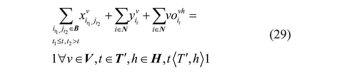
The constraints given in Equation 29 are modified from those given in Equation 13, which indicate that ATs can only have one out of three statuses: going to the next destination, parking at the current node or driving on a trip from the previous horizon,

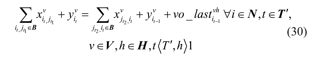
\begin{array}{l} \sum_{\begin{matrix} i_{t_{1},} j_{t_{2}} \in B \\ t_{1} \leq t, t_{2} > t \end{matrix}} x_{i_{t_{1},} j_{t_{2}}}^{v} + \sum_{i \in N} y_{i_{t}}^{v} + \sum_{i \in N} v o_{i_{t}}^{v h} = \\ 1 \forall v \in V, t \in T^{'}, h \in H, t 〈 T^{'}, h 〉 1 \end{array}

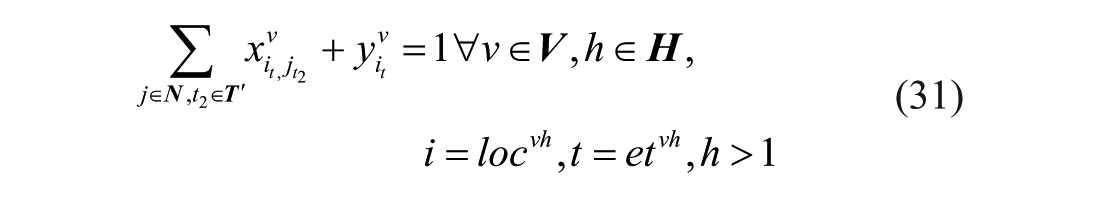
The constraints given in Equation 30 are an updated version of those given in Equation 14. Vehicles arriving at $i_{t}$ are not only from the trip in the current horizon, but also from the previous horizon:

\begin{array}{l} \sum_{i_{t,} j_{t_{1}} \in B} x_{i_{t,} j_{t_{1}}}^{v} + y_{i_{t}}^{v} = \sum_{j_{t_{2},} i_{t} \in B} x_{j_{t_{2},} i_{t}}^{v} + y_{i_{t - 1}}^{v} + v o_l a s t_{i_{t - 1}}^{v h} \forall i \in N, t \in T^{'}, \\ v \in V, h \in H, t 〈 T^{'}, h 〉 1 \end{array}

The constraints given in Equation 31 impose that all the vehicles must start from the same location as they end in the previous horizon:

\begin{array}{l} \sum_{j \in N, t_{2} \in T^{'}} x_{i_{t,} j_{t_{2}}}^{v} + y_{i_{t}}^{v} = 1 \forall v \in V, h \in H, \\ i = l o c^{v h}, t = e t^{v h}, h > 1 \end{array}

The constraints given in Equation 32 guarantee that the half executed requests in the last horizon must be served by the same vehicle in the current horizon:

\begin{array}{l} S_{i j}^{e v} = 1 \forall e \in E 1, h \in H, i = o r i^{e h}, \\ j = d e s^{e}, v = v s^{e h}, h > 1 \end{array}

Case Study and Results

The model is applied to the case-study city of Delft, which is located in the Netherlands, having a total area of 24 km², and a population of about 100,000.

Demand

To apply the model for studying the ATs system in the city of Delft, the following data are needed:

1. The information of the requests;

2. The price and cost of running the system;

3. The road network information of Delft.

The mobility data were obtained from the Dutch mobility dataset (MON 2007/2008) and transformed in the study of Correia and van Arem ( 9 ). These data include the origin and destination, travel mode, departure and arrival time, which is the required information to apply the model in this paper and can be freely obtained online ( 16 ).

The survey sample includes 68,640 requests which were made by residents who travelled only within the city of Delft during the surveyed day. For this application, only the trips done by cars and taxis are considered. A total of 22,240 trips resulted which are represented by 1112 requests in the operation day (expansion coefficient $μ = 20$ ). At the same time, each one of the ATs in our system represents 20 vehicles therefore a taxi satisfying a trip represents 20 taxis satisfying 20 requests. In these experiments, 50% of all the requests are considered to be booked in advance (reserved requests), while 50% are real-time requests. Monte Carlo simulation is used to decide which requests are pre-booked and which are real-time. The original origin and destination, as well as the desired departure time recorded in the data base are used as preferred in the experiments.

According to the time distribution of all the requests, the earliest trip started at 06:48 and the latest trip at 23:35. 06:30–24:00 is chosen as the operation period of the ATs service. The time step of the optimization is 2.5 min. Each horizon contains 12 time steps ( $t_{h} = 12$ ) and the rolling length is 6 time steps ( $t_{r} = 6$ ). In practice this means that at each time the system looks forward to the requests in the next 30 min and updates the ATs’ status every 15 min. This also means the real-time requests will wait 15 min as the maximum waiting time.

The cost values considered are as follows:

$P r$ = 10 € / time step.

$C_{f u e l}$ = 0.1 € / km.

$C_{d}$ = 17.5 € / day.

$ρ_{1}$ = 5 € / trip

$ρ_{2}$ = 2 € / trip

$C_{w}$ = 0.1 € / time step

The penalty for unsatisfied reserved and real-time requests are given different values, which is mainly because the system should give priority to reservations.

The parking outside of Delft city center is free of charge. ATs cannot park in the city center (nodes 28, 4, 3, 44 and 9), but they are able to deliver passengers there and leave immediately. This is based on the parking regulations in the city of Delft.

Road Network

The network has 66 road links and 46 nodes. Some of the links have one lane per way and some have two lanes. The capacities were considered as 1600 and 3200 vehicles per hour per direction based on the number of lanes on that link. The maximum speeds were assumed to be 50 and 70 km/h, respectively, for the lower and higher capacity links.

The minimum travel time $δ_{i j}^{m i n}$ on link (i, j) is obtained from the free flow speed. The maximum travel time $δ_{i j}^{m a x}$ in time step is computed based on the speed of 5 km/h. Travel time at break-point $k$ in time step $δ_{i j}^{k}$ is considered as a function of the traffic flow, which is reflected by the value of break-point $k$ . There are three break-points for the road links with lower capacity and six break-points with higher capacity. These travel times are obtained based on the Bureau of Public Roads function ( 17 ) in equation $t = t_{0} (1 + a \times {(\frac{V}{Q})}^{b})$ , where $t_{0}$ is the minimum travel time, $\frac{V}{Q}$ is the value of break-point $k$ , $a$ is $(δ_{i j}^{m a x} / δ_{i j}^{m i n}) - 1$ and b is 4.

The shortest travel time between the nodes (only for which there is demand) is computed by the shortest path method with free flow travel time ( $O p t_{i j}$ ). The travel distance on each link is the link length in reality.

Results

The optimization model was run in an i5 processor @3.10 GHz, 12.00 GB RAM computer under a Windows 7 64-bit operating system by Xpress, an optimization tool that uses advanced branch-and-cut algorithms for solving integer programming problems.

Two kinds of scenarios are considered. The first one, which is called dynamic travel time, considers the travel time as a function of the taxis traffic flow on each link, as formulated in Equations 18 –20. The second scenario assumes that the travel times do not change and are thus always equal to the minimum travel time on that link, even if the traffic flow varies (static travel times). Therefore, the travel time constraints are turned off. Another key variable for creating these scenarios is the fleet size which represents the number of ATs available in the system.

A comparison of the routing optimization of ATs between different scenarios was performed and is presented in Table 1. The fleets with 100, 200, 300, 400, and 500 ATs are represented by 5, 10, 15, 20, and 25 ATs in the optimizing process, with the expansion coefficient $μ = 20$ . Congestion delay is calculated as the time difference between the real travel time and the shortest travel time of a request. The waiting time is only generated by the real-time requests, which is the difference between the desired departure time and the departure time that the traveler experienced.

Table 1.

Optimization Model Results

	Scenario	Fleet size	Daily profit (×10³ €)	Satisfied requests	Satisfied rate	Satisfied rate of reserved requests	Satisfied rate of real-time requests	Avg. satisfied requests per vehicle	Avg.idle time min/veh.	Avg. travel time min/veh.	Idle rate	Avg. travel distance km/veh.	Avg. congestion delay min/satisfied requests	Avg. waiting time min/satisfied real-time requests
Dynamic travel time	1	100	52.2	1840	8%	13%	3%	18.4	459.0	591.0	44%	257.0	3.5	13.8
	2	200	172.4	3640	16%	28%	5%	18.2	506.3	543.8	48%	229.3	2.2	13.5
	3	300	218.6	4660	21%	32%	10%	15.5	535.0	515.0	51%	210.3	3.7	12.7
	4	400	256.9	5440	24%	35%	14%	13.6	624.1	425.9	59%	172.3	2.9	12.2
	5	500	260.2	5760	26%	35%	16%	11.5	672.4	377.6	64%	149.5	3.2	12.9
Static travel time	6	100	55.6	1900	9%	14%	3%	19.0	510.5	539.5	49%	236.9	-	13.7
	7	200	170.8	3700	17%	28%	5%	18.5	521.3	528.8	50%	225.2	-	12.9
	8	300	273.0	5360	24%	41%	7%	17.9	519.2	530.8	49%	222.1	-	13.2
	9	400	333.6	6680	30%	47%	13%	16.7	560.8	489.3	53%	204.9	-	13.3
	10	500	406.5	8220	37%	55%	19%	16.4	578.6	471.4	55%	196.9	-	12.7

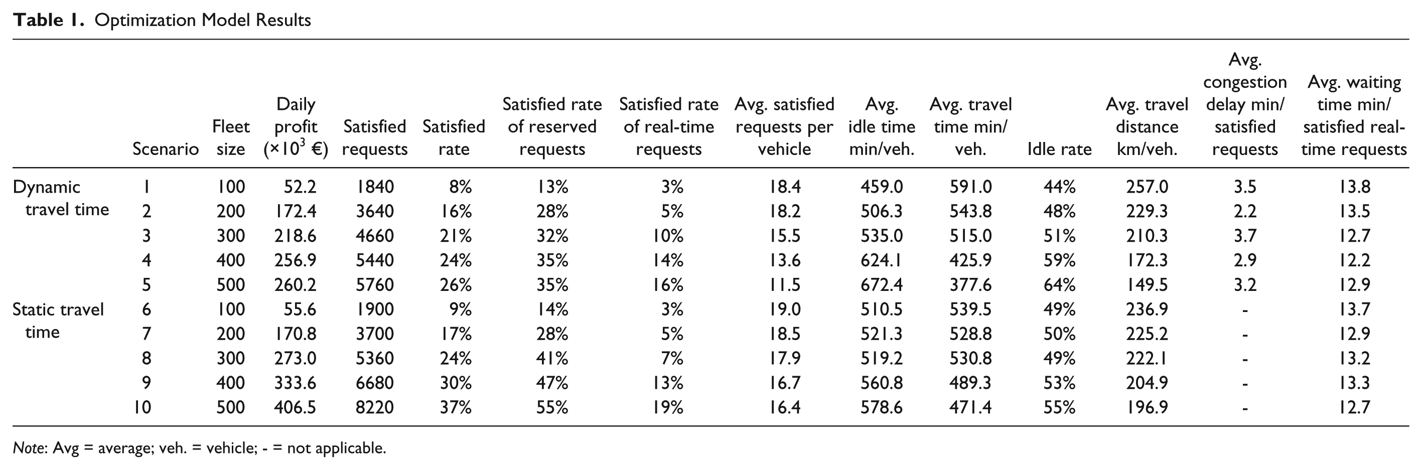
Note: Avg = average; veh. = vehicle; - = not applicable.

In the dynamic travel time scenarios, the fleet size is a critical parameter with respect to the system performance. The daily profit is sensitive to the number of requests satisfied by ATs. When there are only 100 vehicles in the taxi system 1840 requests are satisfied in total. In this case, the satisfied rate is the lowest among all the scenarios. When the fleet size increases to 200, the satisfied demand almost doubled, which also leads to a big increase in the system benefits. This trend continues in scenarios 3, 4 and 5 with 300, 400, and 500 ATs. However, the growth rate is falling in these three scenarios, especially when the fleet size reaches 500. Even though, with more vehicle depreciation cost and less working efficiency, scenario 5 with 500 ATs is the most profitable one among these scenarios with dynamic travel time.

As the penalty of reserved requests is higher than the real-time ones, the system decides to serve reserved requests as a priority. For example, when there are 300 ATs available, 32% of reserved requests are served, while 10% real-time requests are satisfied. As the value of penalty costs has a big influence on deciding which requests are to be served. It also reveals that the system can use this method to adjust the service strategy for different kinds of demand.

The average number of satisfied trips indicates the working efficiency of each AT. In the first five scenarios with dynamic travel time, the most efficient is the one with 100 ATs, with 18.4 requests per vehicle. This also can be seen from the column “average travel time,” “average idle time,” “idle rate,” and “average travel distance.” Scenario 5 has the highest idle time and idle rate. This means more than half of the total operation time ATs are parking somewhere without any movement. The average travel distance is 149.5 km per AT, which is also lower than in any other scenario with the dynamic travel time condition. Actually, it does not conflict with the unsatisfied request rate. The demand is not uniformly distributed during the day which brings out the peak horizons and the off-peak horizons. In the off-peak horizons, 500 ATs are redundant and generate idle time, while in peak horizons there are not enough to serve all the requests.

In the static travel time scenarios, the same trend can be found from scenarios 6 to 10 with regards to the total profitability. Scenario 10 with 500 vehicles has the highest profit, which serves the most requests with a 37% satisfied rate. When the fleet size is 100, each of the ATs are more efficient, serving 19.0 requests in average. The travel distance is also the highest, 236.9 km per vehicle. When the number of ATs decreases, the transport efficiency decreases.

Comparing the static travel time scenarios with dynamic ones, it is easy to find that the ATs system is always more profitable when considering the minimum travel times. When the fleet size is 100, the system obtains 52,200 € under the dynamic travel time condition, which is 6.1% lower than the static travel time with 55,600 €. In addition, the number of satisfied trips in the dynamic travel time scenarios is also less than the one from the static travel time scenarios. The differences in service performance are more obvious in other fleet size scenarios. With 300 ATs, scenario 3 has 19.9% less profit, while with 500 ATs the dynamic travel time scenario has 36.0% less daily profit. This is because when the travel time is always the minimum value, the system would take less time than the dynamic travel time scenario, which makes it possible for the ATs to serve more trips and receive more profit. However, it cannot reflect the real traffic status and the impact of ATs on travel time. This can be seen from the column “Total congestion delay” and the “Avg. congestion delay” in Table 1, which represents the difference between the real travel time and the shortest travel time. These time steps are caused by the traffic congestion and decrease the available service time of ATs.

Conclusion

This paper proposed a mathematical model to study a dynamic travel time based ATs system to provide transport service within the city area. This model involves both the reserved requests and real-time requests by the rolling horizon scheme and optimizes the vehicle routing horizon by horizon. The contribution of this paper is to consider the travel time on each road link according to the number of vehicles travelling on it and perform system optimization with the objective to maximize the total profit of such a system by deciding on each ATs routing selection. It also establishes a rolling horizon scheme to deal with the dynamic vehicle routing problem including real-time information. The model was then applied to a case study in the city of Delft, the Netherlands with a 17.5 hours service period and 23,340 travel requests generating from the road network with 46 nodes and 66 links. From that application it was possible to draw the following conclusions.

The fleet size is an important factor on system profitability, regardless of the dynamic or static travel time. The reason is that more ATs are able to serve more requests which bring more income for the ATs system, even though the depreciation costs are also increasing and the service efficiency is decreasing.

Knowing that real-life travel conditions have dynamic travel time, application of a static minimum travel time vehicle routing model will overestimate the system profitability. Traffic congestion happens when vehicles are travelling on the network, and it leads to less profit, arrival delay and fewer satisfied requests than in the case of the static travel time. However, it reflects the real traffic situation and makes the routing results more realistic.

The influence of considering travel time as dynamic in ATs vehicle routing problems can be seen from two aspects: the time delay on the congested road links and the extra travel distance caused by detouring.

Footnotes

Acknowledgements

The authors would like to thank FICO (Xpress supplier) for establishing a research agreement with the Department of Transport & Planning at TU Delft. This work was supported by ProRail, the train infrastructure manager of the Netherlands. Thanks go also to the Chinese Scholarship Council for sponsoring the first author.

The Standing Committee on Emerging and Innovative Public Transport and Technologies (AP020) peer-reviewed this paper (18-01038).

References

Bose

Ioannou

P. A.

Analysis of Traffic Flow with Mixed Manual and Semiautomated Vehicles. IEEE Transactions on Intelligent Transportation Systems, Vol. 4, No. 4, 2003, pp. 173–188.

Calvert

S. C.

Van Den Broek

T. H. A.

Van Noort

Modelling Cooperative Driving in Congestion Shockwaves on a Freeway Network. Proc., 14th IEEE Intelligent Transportation Systems Conference, ITSC, Washington, D.C., 2011, pp. 614–619.

van Arem

Van Driel

C. J. G.

Visser

The Impact of Cooperative Adaptive Cruise Control on Traffic-Flow Characteristics. IEEE Transactions on Intelligent Transportation Systems, Vol. 7, No. 4, 2006, pp. 429–436.

CityMobil2. CityMobil2 - Cities Demonstrating Automated Road Passenger Transport. http://www.citymobil2.eu/en/.

WEpods. WEpods project DAVI – Dutch Automated Vehicle Initiative. http://davi.connekt.nl/wepods-project/.

Martinez

L. M.

Correia

G. H. A.

Viegas

J. M.

An Agent-Based Simulation Model to Assess The Impacts of Introducing a Shared-Taxi System: An Application to Lisbon (Portugal). Journal of Advanced Transportation, Vol. 49, No. 1, 2015, pp. 475–495.

Spieser

Treleaven

Zhang

Frazzoli

Morton

Pavone

Toward a Systematic Approach to the Design and Evaluation of Automated Mobility-on-Demand Systems: A Case Study in Singapore. In Road Vehicle Automation ( Meyer

Beiker

, eds.), Springer, New York, 2014, pp. 229–245.

Liang

de Almeida Correia

G. H.

van Arem

Optimizing the Service Area and Trip Selection of an Electric Automated Taxi System Used for the Last Mile of Train Trips. Transportation Research Part E: Logistics and Transportation Review, Vol. 93, 2016, pp. 115–129.

de Almeida Correia

G. H.

van Arem

Solving the User Optimum Privately Owned Automated Vehicles Assignment Problem (UO-POAVAP): A Model to Explore the Impacts of Self-Driving Vehicles on Urban Mobility. Transportation Research Part B: Methodological, Vol. 87, 2016, pp. 64–88.

10.

Levin

M. W.

Congestion-Aware System Optimal Route Choice for Shared Autonomous Vehicles. Transportation Research Part C: Emerging Technologies, Vol. 82, 2017, pp. 229–247.

11.

Psaraftis

H. N.

Dynamic Vehicle Routing Problems. In Vehicle Routing: Methods and Studies ( Golden

B. L.

Assad

A. A.

, eds.), North Holland, Amsterdam, The Netherlands, 1988, pp. 223–248.

12.

Mitrović-Minić

Krishnamurti

Laporte

Double-Horizon Based Heuristics for the Dynamic Pickup and Delivery Problem with Time Windows. Transportation Research Part B: Methodological, Vol. 38, No. 8, 2004, pp. 669–685.

13.

Yang

Jaillet

Mahmassani

On-Line Algorithms for Truck Fleet Assignment and Scheduling Under Real-Time Information. Transportation Research Record: Journal of the Transportation Research Board, 1999. 1667: 107–113.

14.

Luo

Schonfeld

Online Rejected-Reinsertion Heuristics for Dynamic Multivehicle Dial-a-Ride Problem. Transportation Research Record: Journal of the Transportation Research Board, 2011. 2218: 59–67.

15.

Kaufman

D. E.

Nonis

Smith

R. L.

A Mixed Integer Linear Programming Formulation of the Dynamic Traffic Assignment Problem. Proc., IEEE International Conference on Systems, Man and Cybernetics, Chicago, Illinois, Vol. 1, 1992, pp. 232–235.

16.

Correia

G. H. de A.

van Arem

Trips and network of the case-study city of Delft. https://www.researchgate.net/publication/309134999_Trips_and_network_of_the_case-study_city_of_Delft

17.

Dafermos

Sparrow

Traffic Assignment Problem for a General Network. Journal of Research of the National Bureau of Standards B, Vol. 73, No. 2, 1969, pp. 91–118. http://www.scopus.com/inward/record.url?eid=2-s2.0-0014491807&partnerID=tZOtx3y1.

Applying a Model for Trip Assignment and Dynamic Routing of Automated Taxis with Congestion: System Performance in the City of Delft,The Netherlands

Abstract

Integer Programming Model

Sets

Data

Parameters

Decision Variables

Objective Function

Subject to the Following Constraints

Rolling Horizon

Rolling Horizon Scheme

Demand Initialization

Continuity

Case Study and Results

Demand

Road Network

Results

Conclusion

Footnotes

Acknowledgements

References