Sage Journals: Discover world-class research

Abstract

This study investigates the influence of firm-idiosyncratic profitability on stock pricing decisions and whether a trading strategy based on idiosyncratic profitability can generate significant hedge portfolio abnormal returns. We disaggregate a firm’s profitability into three components—a market component, an industry component, and a firm-specific component, which we label as idiosyncratic profitability. We document that a trading strategy based on idiosyncratic profitability generates significant hedge portfolio returns. Our results are robust in that our hedge portfolio returns still exist after controlling for known risk factors and previously documented anomalies.

JEL Classifications: C58; G11; G14; M20; M41

Keywords

Abnormal returns idiosyncratic industry market pricing profitability trading strategy

1. Introduction

Examining whether market participants fully appreciate the implications of firm strategy on reported profitability is an important question, as it tests the ability of investors to understand the aspects of firm performance under the direct control of management.¹ This is especially important given that the market regularly discounts the uniqueness of a firm’s strategy (Litov et al., 2012). We use the method in Jackson et al. (2018) to disaggregate a firm’s profitability into three components—a market component, an industry component, and a firm-specific component, which we label as idiosyncratic profitability. Following the rationale behind the Jackson et al. (2018) disaggregation method, we view the idiosyncratic component of profitability as representing the ex post earnings outcome of a firm’s strategic response to the competitive pressures within the industry and general macroeconomic conditions.²

We expect to observe a significant association between idiosyncratic profitability and stock returns that results from investors making systematic expectation errors (Bouchaud et al., 2019) because investors do not fully understand the implications of a firm’s strategy and thus its idiosyncratic profitability.³ Accordingly, the construction of a hedge portfolio trading strategy based on the level of a firm’s idiosyncratic profitability may be able to generate significant abnormal returns. Therefore, we examine the influence of the firm-idiosyncratic component of profitability on stock pricing decisions and whether a trading strategy based on the idiosyncratic component can be used to generate significant hedge portfolio abnormal returns.

For firms able to successfully implement their strategies and establish competitive advantages, we expect the idiosyncratic component of profitability to be greater.⁴ As a result, taking a long position in firms with high values of this component should generate positive returns, as less informed investors will learn that earnings for these firms will be higher than expected if based on market and industry expectations. On the other hand, a negative value of idiosyncratic profitability implies a less than successful firm strategy, and profitability will be lower than expected.⁵ In essence, the firm is unable to capitalize on any competitive advantages, which reduces idiosyncratic profitability. This explanation is consistent with the arguments of Hui et al. (2016) that competition erodes competitive advantages so that any positive abnormal returns are not expected to be sustainable in the long run. The market and industry components of profitability, by sharing common information across all market and industry participants, respectively, are expected to be associated with common price movements. To the extent that common market information is embedded in prices as other firms announce their earnings (Jackson et al., 2020), it is the firm-specific component that provides information that is not already incorporated into prices, thus causing price movements.

Our approach is related to the profitability anomalies of Novy-Marx (2013) and Hou et al. (2015). Hou et al. (2015) include a profitability factor based on Return on Equity (ROE) based on a q-theory of investment. They argue that ROE predicts returns because high (low) expected ROE relative to investment implies a high (low) discount rate. High discount rates are necessary to offset the high expected ROE to induce low net present values of new capital and low investment. Novy-Marx (2013), on the other hand, identifies that controlling for profitability dramatically increases the performance of value trading strategies and explains most earnings-related anomalies and a wide range of seemingly unrelated profitable trading strategies. Our study differs from anomalies popularized by Novy-Marx (2013) and Hou et al. (2015) in that we use the method in Jackson et al. (2018) to disaggregate a firm’s profitability into market, industry, and idiosyncratic components.

Our results show that, on average, significant positive hedge returns can be earned by taking a long (short) position in firms with higher (lower) levels of the firm-idiosyncratic component of earnings, with the mean value-weighted hedge portfolio returns based on idiosyncratic return on assets (IdiosROA) generated returns of 0.66% per month, and 1.23% per month in the first month after the information to conduct the disaggregation procedure is possible. Further, hedge portfolio alphas of at least 0.59% in excess of the Hou et al. (2015) factors are able to be generated.

Our results are robust in that our hedge portfolio returns still exist after controlling for known risk factors and previously documented anomalies. Using an online tool provided by Mihail Velikov,⁶ we are able to show in an Online Appendix that using idiosyncratic profitability is able to add to the “factor zoo.” Of specific note, after accounting for trading costs, our strategy ranks between the 95^th and 99^th percentiles in terms of how much it could have expanded the achievable investment frontier relative to the other 212 anomalies identified in the online tool (Novy-Marx and Velikov, 2024). We also document that there are no hedge portfolio returns to a trading strategy based on the market or industry components of profitability. Overall, our findings are consistent with either investors not fully understanding the implications of the market, industry, and idiosyncratic components of profitability or idiosyncratic profitability being correlated with an unmodeled risk factor not previously identified in the literature (Landsman et al., 2011).

The main contribution of our study is documenting that predictable abnormal returns can be generated using a trading strategy based on ranking firms according to the level of their idiosyncratic profitability. Our approach differs from anomalies popularized by Novy-Marx (2013) and Hou et al. (2015) by interpreting the firm’s idiosyncratic profitability as representing the outcome of a firm’s strategic response to the competitive pressures within the industry and general macroeconomic conditions. The approaches in both Hou et al. (2015) and Novy-Marx (2013) are consistent with fundamental analysis, which involves analyzing both specific ratios and how a firm compares to its competitors and industry peers in order to more accurately predict future outcomes. Hou et al. (2015) use an ROE factor in their asset pricing model, which, while it is a useful summary measure, does not explain the uniqueness of those profits compared to industry peers. The Novy-Marx (2013) gross profitability factor is one manner in which the operating management of the firm is able to be assessed as a driver of profitability, but this does not capture the uniqueness of those profits compared to industry peers. We use return on assets (ROA) as a profitability ratio that is commonly used in fundamental analysis, but our approach disaggregates that ratio into market, industry, and idiosyncratic components. This allows us to capture the firm-specific component of a firm’s profitability, that is its unique component that reflects the outcome of its strategy. Therefore, we contribute to the literature by utilizing a method where we are able to assess where firms have been able to utilize their competitive advantage to generate profitability in excess of market and industry factors, that is the idiosyncratic component of profitability, which is the unique firm-specific component of profitability.

Our study further contributes to the literature in the following way. Prior research focuses on the industry-specific and idiosyncratic components of profitability, assuming that the industry component for all firms will be the average earnings within the industry-quarter, with the idiosyncratic component being the remainder (Hui and Yeung, 2013; Hui et al., 2016). Our approach explicitly models a firm’s profitability to be comprised of market-wide, industry-specific, and idiosyncratic profitability, allowing for cross-sectional variation in the components by allowing for historical sensitivities of a firm’s profitability to the market and industry, thus better capturing the idiosyncratic component. By more accurately capturing the idiosyncratic component of a firm’s profitability, we are able to document significant hedge portfolio returns by trading on an economically meaningful component of a firm’s profitability, that is its profitability capturing the outcome of the implementation of firm strategy, as opposed to a statistical observation. Our study also enhances our understanding of stock return predictability, which is a fundamental topic in financial economics (Dong et al., 2022). The observed results provide valuable insights into the interplay between profitability components and investor behavior, enriching the discourse of financial economics.

2. Related literature

Prior research shows that disaggregating a firm’s profitability into market, industry, and firm-idiosyncratic components improves the accuracy of a firm’s profitability forecasts (Jackson et al., 2018). In addition, the general economy (the industry and market) components of profitability and the firm-idiosyncratic component of profitability exhibit differential persistence (Hui et al., 2016; Jackson et al., 2018) and therefore should be weighted differently by market participants when valuing a firm’s future performance. If the market is perfectly efficient, investors should fully anticipate the information contained in the different components of a firm’s profitability and correctly value the firm. However, prior research finds that the market is not always perfectly efficient (Bernard and Thomas, 1990; Jegadeesh and Titman, 1993; Lakonishok et al., 1994; Shiller et al., 1984), and investors may not fully use available information about a firm’s profitability when making their pricing decisions (Hui et al., 2016; Sloan, 1996; Vorst and Yohn, 2018).

Prior research on disaggregating profitability into common industry and market components generally assumes an average amount of market- and industry-related information for each firm, which holds the market portion, industry portion, or both components of earnings cross-sectionally constant from firm to firm (see, e.g. Ayers and Freeman, 1997; Hui and Yeung, 2013; Hui et al., 2016). In contrast, Jackson et al. (2018) disaggregate a firm’s profitability into market, industry, and firm-idiosyncratic components and allow cross-sectional variation in the market and industry components of a firm’s profitability. Jackson et al. (2018) initial test on the accuracy of their earnings disaggregation model reveals that the quarterly persistence of each component of a firm’s profitability is different from the quarterly persistence of total profitability. The market (firm-idiosyncratic) component exhibits the strongest (weakest) persistence parameter of the three components of earnings. The differential quarterly persistence of each earnings component estimated in Jackson et al. (2018) implies that market participants can make more accurate forecasts of a firm’s earnings by placing different weights on each earnings component.

With respect to the market and industry components of a firm’s profitability, external users have access to a wide variety of macroeconomic indicators and industry-level information that are easy to verify, which in turn reduces uncertainty around earnings expectations at the firm level. In contrast, with respect to the idiosyncratic component of a firm’s profitability, external users will face difficulties in forming robust expectations as it is more difficult to verify (Jackson et al., 2025) and less persistent compared to the market and industry components of earnings (Jackson et al., 2018). These characteristics of idiosyncratic earnings make it more difficult for investors to price, thus leading to the construction of a hedge portfolio trading strategy based on the level of a firm’s idiosyncratic profitability that may be able to generate significant abnormal returns. This logic is similar to the differential persistence of cash flows (easy-to-verify) and accruals (difficult-to-verify) that is the basis of the Sloan (1996) accruals anomaly.

Economic theory on the competitive environment suggests that a firm’s earnings that are consistent with the industry norm are relatively more persistent because below-average performers can learn from other competitors and that the learning effect erodes the competitiveness of leading performers (Hui et al., 2016; Mueller, 1977; Waring, 1996). The industry norm is determined by various industry characteristics, such as production technology and the tastes of consumers, which can influence the performance of all firms in the same industry (Mueller, 1977; Hui et al., 2016). Therefore, competition and a firm’s learning behavior erode a firm’s idiosyncratic performance that deviates from the standard performance of the industry and cause a firm’s earnings associated with its idiosyncratic performance to revert quickly. This implies that the component of a firm’s profitability that is attributable to a firm’s idiosyncratic performance is less persistent than that attributable to industry and market effects, as demonstrated by Jackson et al. (2018).

Capital markets have been shown to systematically discount uniqueness in a firm’s strategic choices (Litov et al., 2012). The cost of collecting and analyzing information to evaluate a firm’s future value is increasing in its uniqueness. These increased costs discourage private information searches regarding the firm, leading to undervaluation. In the extreme, market participants may find the effort necessary to investigate a firm’s strategy simply too great to justify (Veldkamp, 2006). On the other hand, uniqueness in strategy is seen as a necessary condition for creating economic rents and should be positively associated with firm value. Therefore, from a fundamental analysis perspective, it would be expected that returns will be higher (lower) for firms who are able (unable) to successfully implement their strategy, that is firms with higher (lower) idiosyncratic profitability.

3. Research design

3.1. Earnings disaggregation

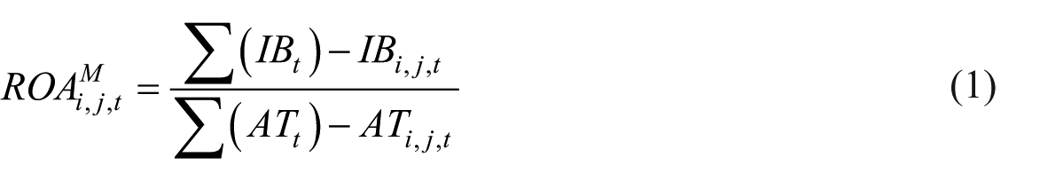
To improve the accuracy of a firm’s profitability forecasts, Jackson et al. (2018) disaggregate a firm’s profitability into market, industry, and firm-idiosyncratic components by adapting the earnings beta estimation technique in Beaver et al. (1970) and Jackson et al. (2017). We use ROA, calculated as income before extraordinary items (Compustat item IB) scaled by average total assets (Compustat item AT)) as a commonly used measure of earnings by market participants to analyze a firm’s performance.⁷ We follow the approach in Jackson et al. (2018) to empirically classify firm profitability into its market (MktROA), industry (IndROA), and idiosyncratic (IdiosROA) components. The Jackson et al. (2018) disaggregation method uses the past 20 quarters (with a minimum of 10 observations required) of earnings information to estimate earnings betas, which then allows for cross-sectional variation within periods for both the market and industry portions of earnings. In contrast, other approaches assume that the market and industry portions of earnings are a cross-sectional constant each period, thus constraining firms to have the same level of market and industry earnings. Firms are expected to be differentially sensitive to market and industry factors, as demonstrated by Jackson et al. (2017), questioning the appropriateness of this approach. The Jackson et al. (2018) measure relaxes this strong assumption, making it more consistent with the long line of finance literature that examines the sensitivity of firm stock returns to market and industry factors.

To disaggregate a firm’s ROA, the market-level ROA and industry-level ROA need to be calculated first. These market- and industry-level ROAs are calculated on a firm-quarter basis. Following Jackson et al. (2018), market-level ROA ( $R O A_{i, j, t}^{M}$ ) is calculated as the sum of income before extraordinary items (IB) divided by the sum of average total assets (AT) across all firms included in Compustat for quarter t, excluding firm i⁸

\begin{matrix} R O A_{i, j, t}^{M} = \frac{\sum (I B_{t}) - I B_{i, j, t}}{\sum (A T_{t}) - A T_{i, j, t}} \end{matrix}

(1)

The estimation of the market-level ROA explicitly excludes the firm itself to mitigate concerns about heavier weights being applied to larger firms.

Industry ROA ( $R O A_{i, j, t}^{I}$ ) is calculated as the sum of IB divided by the sum of AT within industry j defined by six-digit GICS codes⁹ for quarter t, excluding firm i

\begin{matrix} R O A_{i, j, t}^{I} = \frac{\sum (I B_{j, t}) - I B_{i, j, t}}{\sum (A T_{j, t}) - A T_{i, t j,}} \end{matrix}

(2)

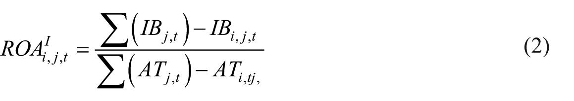
Similar to the calculation of the market-level ROA, we explicitly exclude the firm itself from the calculation of a firm-specific industry ROA.

The measures of market-level ROA ( $R O A_{i, j, t}^{M}$ ) and industry ROA ( $R O A_{i, j, t}^{I}$ ) are then used to estimate the industry and market betas. First, to measure industry profitability that is orthogonal to market profitability, we conduct regressions using $R O A^{I}$ as the dependent variable and $R O A^{M}$ as the independent variable and take the residual (ε) in equation (3) as the measure of industry ROA, consistent with the methodological approach in Brown and Ball (1967). This step excludes the market effects from the industry component and attributes the common information between the industry and market to the market component. Second, we conduct regressions with a firm’s total ROA as the dependent variable and market ROA and the industry ROA as independent variables, excluding the market effect, and take ${β^{'}}_{1}$ and ${β^{'}}_{2}$ in equation (4) to be the estimated industry and market earnings quarterly betas that capture the sensitivity to market and industry earnings

\begin{matrix} R O A_{i, j, t}^{I} = β_{0} + β_{1} R O A_{i, j, t}^{M} + ϵ \end{matrix}

(3)

\begin{matrix} R O A_{i, j, t} = {β^{'}}_{0} + {β^{'}}_{1} {\hat{ϵ}}_{i, j, t} + {β^{'}}_{2} R O A_{i, j, t}^{M} + ϵ^{'} \end{matrix}

(4)

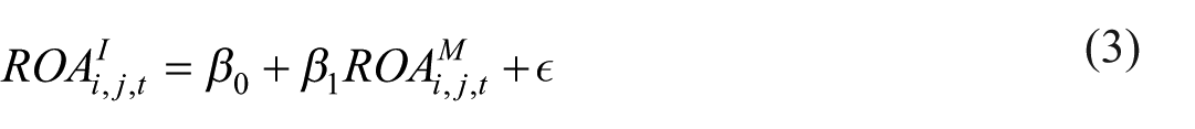
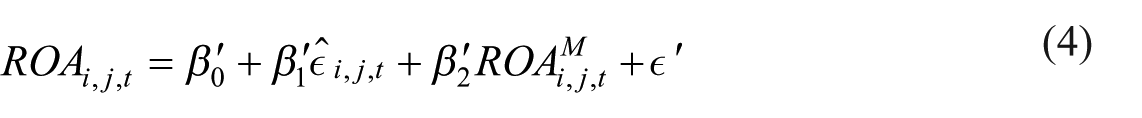
This two-step process allows us to disaggregate a firm’s total ROA into the market, industry, and firm-idiosyncratic components. To calculate estimates of the quarterly market component of ROA ( $M k t R O A_{i, j, t}$ ), the industry component of ROA ( $I n d R O A_{i, j, t}$ ), and the firm-idiosyncratic component of ROA ( $I d i o s R O A_{i, j, t}$ ), we apply the betas from equation (4) to the quarterly $R O A_{t}^{M}$ and $R O A_{j, t}^{I}$ in the following equations

\begin{matrix} M k t R O A_{i, j, t} = {\hat{β^{'}}}_{2} \times R O A_{t}^{M} \end{matrix}

(5)

\begin{matrix} I n d R O A_{i, j, t} = \hat{{β^{'}}_{1}} \times R O A_{j, t}^{I} \end{matrix}

(6)

\begin{matrix} I d i o s R O A_{i, j, t} = R O A_{i, j, t} - M k t R O A_{i, j, t} - I n d R O A_{i, j, t} \end{matrix}

(7)

The Jackson et al. (2018) methodology assumes that information is only attributable to one source and does not simultaneously impact different components, that is it enters in a linear fashion. This approach, however, does not attempt to classify any specific information signal to a particular component but allows for historical sensitivities to provide a disaggregation of the total profitability. As such, it implies that a certain signal may contain market, industry, and idiosyncratic components in a manner which is more complex than a linear model may imply. It does require, though, that the components of profitability do sum to total profitability.

3.2. Sample

Our sample selection proceeds in two steps. First, quarterly data are collected from Compustat to estimate the market, industry, and firm-idiosyncratic components of profitability. Following Jackson et al. (2018), our initial sample selection starts with all firm-quarter observations that have common shares listed on one of the three major U.S. stock exchanges (NYSE, AMEX, or NASDAQ) and a GICS code during the period from 1977 to 2023.

There are some restrictions for the initial sample selection: (1) we only include firms with March, June, September, and December fiscal-quarter ends as in Jackson et al. (2018); (2) we restrict industry-quarters in the sample to have at least five observations per industry-quarter to ensure the industry betas have sufficient statistical power (Bhojraj et al., 2003; Jackson et al., 2018); (3) observations are required to have sufficient data to estimate industry- and market-ROA betas; and (4) we exclude observations with industry or market betas larger than an absolute value of 3 to reduce the noise caused by outliers (Jackson et al., 2018). After collecting all data required from Compustat Fundamentals Quarterly with control and profitability variables, we obtain a sample of 550,668 firm-quarter observations, which reduces to 303,457 after matching with the disaggregated profitability measures.

Second, price and return data are collected from CRSP from 1977 to 2023. The final sample is obtained by merging the initial sample with the CRSP stock files. Our final sample comprises 605,130 monthly returns, based on 201,988 firm-quarter observations from 1977 to 2023. Fama and MacBeth and portfolio tests are based on 531 monthly observations, from 177 unique fiscal quarters.

4. Results

Table 1 provides descriptive statistics for the key variables of interest. In terms of profitability, quarterly ROA has a mean (median) of 0.83% (0.72%), with a standard deviation of 0.0187. After disaggregating annual ROA into its components, quarterly MktROA has a mean (median) of 0.14% (0.06%); quarterly IndROA has a mean (median) of 0.24% (0.08%); and quarterly IdiosROA has the largest components of earnings with a mean (median) of 0.45% (0.33%). The standard deviations of MktROA and IndROA are 0.0070 and 0.0098, respectively, both less than half that of IdiosROA (0.0212). These descriptives of the components of earnings are largely consistent with Jackson et al. (2018), especially in terms of the standard deviations, and consistent with Brown and Ball (1967), that roughly half of a firm’s profitability is firm specific.

Table 1.

Descriptive statistics.

	Mean	Std. Dev.	p1	Q1	Median	Q3	p99
ROA	0.0083	0.0187	-0.0823	0.0020	0.0072	0.0169	0.0580
MktROA	0.0014	0.0070	-0.0171	-0.0016	0.0006	0.0050	0.0199
IndROA	0.0024	0.0098	-0.0850	-0.0299	0.0008	0.0050	0.0396
IdiosROA	0.0045	0.0212	-0.0872	-0.0023	0.0033	0.0142	0.0628
Ret_t	0.0096	0.1185	-0.3197	-0.0524	0.0043	0.0647	0.4317

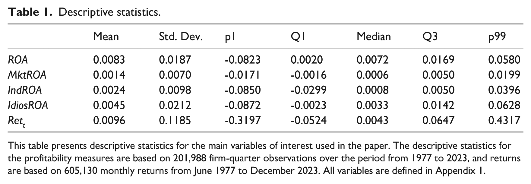
This table presents descriptive statistics for the main variables of interest used in the paper. The descriptive statistics for the profitability measures are based on 201,988 firm-quarter observations over the period from 1977 to 2023, and returns are based on 605,130 monthly returns from June 1977 to December 2023. All variables are defined in Appendix 1.

4.1. Pricing

We examine whether investors’ expectations embedded in stock prices fully reflect the differential persistence attributable to the market, industry, and idiosyncratic components of profitability as documented by Jackson et al. (2018). We use a Fama and MacBeth regression approach using monthly raw returns against quarterly profitability components.¹⁰ Specifically, we allow for two months after the quarter end to allow for all firms to report their quarterly earnings, so that at the end of month + 2 we are able to estimate the profitability components, allowing for monthly returns in month + 3 to + 5 after the quarter end to be matched to quarterly earnings. For example, for the first quarter ending in March, we wait till May to be able to conduct the disaggregation procedure, so we allow for June through August returns to be related to first quarter profitability. We present our results from 531 monthly regressions in Table 2.

Table 2.

Fama and MacBeth regressions of returns on measures of profitability.

	(1)	(2)	(3)
ROA_t	0.312 (1.57)
MktROA_t		0.232(0.80)	1.122(1.53)
IndROA_t		0.410(1.47)	0.720(1.30)
IdiosROA_t		0.396*** (6.07)	0.357*** (3.99)
Growth_t			0.018*** (3.57)
Size_t			0.000(0.42)
BTM_t			-0.002*** (-3.11)
Ret_t-1			-0.052*** (-6.14)
Constant	0.008(4.06)	0.008(4.28)	0.006(1.35)
N	531	531	531
Adj R²	0.014	0.020	0.053

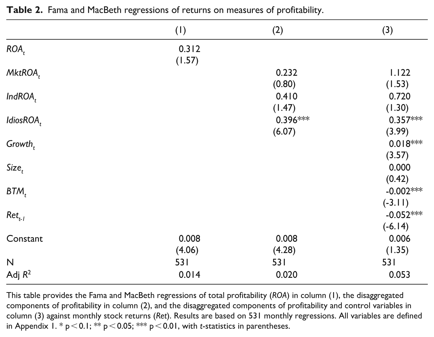
This table provides the Fama and MacBeth regressions of total profitability (ROA) in column (1), the disaggregated components of profitability in column (2), and the disaggregated components of profitability and control variables in column (3) against monthly stock returns (Ret). Results are based on 531 monthly regressions. All variables are defined in Appendix 1. * p < 0.1; ** p < 0.05; *** p < 0.01, with t-statistics in parentheses.

Column (1) of Table 2 presents the results from simply regressing total profitability as the dependent variable, as measured by ROA against monthly returns. Our results indicate that there is no abnormal return available by trading on the level of ROA (0.312, Fama and MacBeth t-stat 1.57). As discussed earlier, total profitability is a summary measure that is not able to capture the nuances in firm performance that can be gleaned from disaggregating this into market, industry, and idiosyncratic components. In column (2), we separate out the total profitability into the market (MktROA), industry (IndROA), and idiosyncratic (IdiosROA) components. Here, we find that IdiosROA is significantly related to monthly returns (0.396, t-stat 6.07) while MktROA and IndROA are not significantly related to monthly returns. Also of importance, we document that the Adjusted R² increases from 1.4% to 2.0% when disaggregating ROA into the three components, indicating that they provide incremental information to the market.

Finally, to address concerns that the significant returns on the idiosyncratic component of earnings are being driven by other known risk factors, we augment our model to include sales growth (Growth), firm size (Size), book to market (BTM), and momentum in stock returns (Ret_t-1). Due to concerns around multicollinearity, we do not include gross profitability (Novy-Marx, 2013) or the earnings-to-price multiple. Our results in column (3) document that IdiosROA remains the only component of profitability that is significantly related to monthly stock returns (0.357, t-stat 3.99). The results are unaffected when controlling for quarterly seasonality.¹¹

4.2. Trading strategy

The pricing results described above suggest that predictable abnormal stock returns can be earned through a trading strategy by taking a hedge portfolio of firms with high and low levels of idiosyncratic profitability. The formation of a trading strategy based on the levels of idiosyncratic profitability is also intuitively appealing, as it captures a firm’s specific response to market and industry conditions and allows us to estimate the economic results of a firm’s strategic decisions.

To test whether predictable returns can be generated by using this trading strategy, we sort firms into quintiles based on the signed magnitude of firm-idiosyncratic profitability at the end of each month. As the disaggregation procedure can be conducted every three months (end of May, August, November, and February), portfolios are rebalanced quarterly. Within each portfolio, we calculated the value-weighted and equal-weighted returns of each portfolio separately in each month in the sample.

In Panel A of Table 3, we present the mean monthly returns for portfolio formation. In doing so, we also consider alternate profitability measures to include ROA, return on net operating assets (RNOA), and ROE. Across all equal-weighted monthly returns, we find significant hedge portfolio monthly returns ranging from 1.24% (t-stat 7.62) for RNOA to 1.43% (t-stat 12.28) for ROE. Using value-weighted portfolio returns, we do not find statistically significant hedge portfolio monthly returns for RNOA (0.39%, t-stat 1.60), but do find significant returns for ROA (0.66%, t-stat 2.62) and ROE (0.73%, t-stat 2.83).¹² While these t-statistics are below 3.0, as the approach we use to justify IdiosROA as a signal is derived from theory, a t-statistic greater than 2.0 is supportive of a significant return (Harvey et al., 2016).

Table 3.

Monthly returns.

Panel A: All Months
	IdiosROA		IdiosRNOA		IdiosROE
	VWRet	EWRet	VWRet	EWRet	VWRet	EWRet
Low	0.0061	0.0045	0.0073	0.0030	0.0055	0.0041
2	0.0109	0.0113	0.0120	0.0112	0.0101	0.0111
3	0.0116	0.0125	0.0126	0.0125	0.0111	0.0121
4	0.0133	0.0137	0.0126	0.0135	0.0142	0.0144
High	0.0126	0.0185	0.0112	0.0154	0.0128	0.0184
High–Low	0.0066(2.62)	0.0139(10.14)	0.0039(1.60)	0.0124(7.62)	0.0073(2.83)	0.0143(12.28)
N	531	531	531	531	531	531
Panel B: First Month Returns
	IdiosROA		IdiosRNOA		IdiosROE
	VWRet	EWRet	VWRet	EWRet	VWRet	EWRet
Low	-0.0009	0.0011	-0.0002	0.0006	-0.0057	0.0006
2	0.0063	0.0089	0.0085	0.0076	0.0070	0.0085
3	0.0027	0.0067	0.0086	0.0076	0.0052	0.0083
4	0.0099	0.0111	0.0088	0.0106	0.0089	0.0103
High	0.0114	0.0173	0.0071	0.0141	0.0111	0.0151
High–Low	0.0123(2.75)	0.0162(8.92)	0.0073(1.95)	0.0135(7.07)	0.0167(3.79)	0.0145(8.36)
N	177	177	177	177	177	177

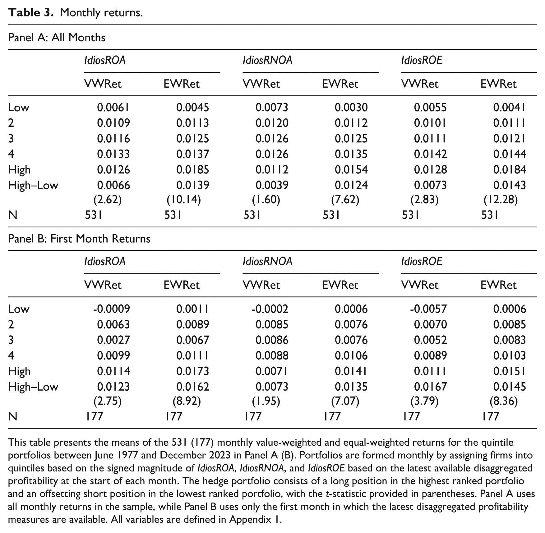
This table presents the means of the 531 (177) monthly value-weighted and equal-weighted returns for the quintile portfolios between June 1977 and December 2023 in Panel A (B). Portfolios are formed monthly by assigning firms into quintiles based on the signed magnitude of IdiosROA, IdiosRNOA, and IdiosROE based on the latest available disaggregated profitability at the start of each month. The hedge portfolio consists of a long position in the highest ranked portfolio and an offsetting short position in the lowest ranked portfolio, with the t-statistic provided in parentheses. Panel A uses all monthly returns in the sample, while Panel B uses only the first month in which the latest disaggregated profitability measures are available. All variables are defined in Appendix 1.

For comparative purposes, we also include in Panel B of Table 4 the monthly hedge portfolio returns for only the first month following portfolio formation. We continue to find similar results, with the exception that the magnitude of the value-weighted returns is around double for all months. We take this as evidence consistent with the notion that investors are able to quickly and accurately reflect firm-specific information into price (Durnev et al., 2004). Accordingly, we continue to take the pooled monthly returns as a baseline result.

Table 4.

Factor returns.

Portfolio	Low	2	3	4	High
Panel A: CAPM Factors
MKT	0.0106*** (21.74)	0.0095*** (26.73)	0.0086*** (28.55)	0.0092*** (34.88)	0.0094*** (33.05)
α	-0.0019(-0.85)	0.0039** (2.45)	0.0051*** (3.76)	0.0065*** (5.49)	0.0056*** (4.44)
Observations	531	531	531	531	531
Adj. R-squared	0.4708	0.5738	0.6043	0.6963	0.6731
Panel B: Fama and French (1993) Factors
MKT	0.0104*** (20.54)	0.0101*** (29.30)	0.0091*** (29.82)	0.0095*** (34.19)	0.0092*** (30.62)
SMB	0.0037*** (5.10)	0.0008* (1.66)	0.0000(0.10)	0.0001(0.27)	-0.0001(-0.26)
HML	0.0027*** (3.76)	0.0050*** (10.32)	0.0033*** (7.69)	0.0018*** (4.51)	-0.0013*** (-3.04)
α	-0.0032(-1.50)	0.0018(1.20)	0.0037*** (2.84)	0.0057*** (4.91)	0.0062*** (4.86)
Observations	531	531	531	531	531
Adj. R-squared	0.5059	0.6455	0.6427	0.7065	0.6776
Panel C: Fama and French (2016) Factors
MKT	0.0103*** (19.41)	0.0100*** (27.63)	0.0094*** (29.78)	0.0097*** (34.01)	0.0093*** (30.04)
SMB	0.0034*** (4.32)	0.0009* (1.74)	0.0007(1.48)	0.0007* (1.65)	0.0006(1.37)
HML	0.0030*** (3.09)	0.0055*** (8.40)	0.0023*** (3.99)	0.0008(1.62)	-0.0015*** (-2.65)
RMW	-0.0013(-1.30)	0.0003(0.43)	0.0024*** (4.07)	0.0022*** (4.10)	0.0026*** (4.54)
CMA	-0.0002(-0.15)	-0.0013(-1.30)	0.0015* (1.76)	0.0013* (1.73)	-0.0005(-0.62)
α	-0.0026(-1.20)	0.0019(1.26)	0.0024* (1.83)	0.0046*** (3.87)	0.0052*** (4.06)
Observations	531	531	531	531	531
Adj. R-squared	0.5056	0.6455	0.6535	0.7155	0.6892
Panel D: Fama and French (2016) Factors with Momentum
MKT	0.0098*** (18.53)	0.0098*** (26.73)	0.0094*** (29.02)	0.0096*** (33.02)	0.0094*** (29.52)
SMB	0.0036*** (4.67)	0.0010* (1.96)	0.0007(1.56)	0.0008* (1.87)	0.0006(1.33)
HML	0.0017* (1.72)	0.0049*** (7.15)	0.0021*** (3.44)	0.0004(0.68)	-0.0014** (-2.38)
RMW	-0.0009(-0.92)	0.0005(0.70)	0.0025*** (4.16)	0.0023*** (4.37)	0.0026*** (4.48)
CMA	0.0009(0.60)	-0.0008(-0.77)	0.0017* (1.94)	0.0017** (2.22)	-0.0006(-0.68)
MOM	-0.0020*** (-4.00)	-0.0010*** (-2.78)	-0.0003(-1.12)	-0.0008*** (-2.75)	0.0001(0.41)
α	-0.0014(-0.63)	0.0025* (1.66)	0.0026** (1.97)	0.0051*** (4.25)	0.0051*** (3.95)
Observations	531	531	531	531	531
Adj. R-squared	0.5194	0.6500	0.6536	0.7190	0.6887
Panel E: Hou et al. (2015) Factors
MKT	0.0099*** (18.27)	0.0098*** (24.62)	0.0091*** (27.25)	0.0095*** (31.93)	0.0095*** (29.57)
ME	0.0027*** (3.54)	0.0007(1.17)	0.0001(0.22)	0.0003(0.67)	0.0005(1.06)
IA	0.0024** (2.35)	0.0039*** (5.14)	0.0039*** (6.00)	0.0024*** (4.18)	-0.0016** (-2.56)
ROE	-0.0041*** (-4.21)	-0.0011(-1.55)	0.0017*** (2.90)	0.0014** (2.53)	0.0025*** (4.40)
EG	0.0005(0.42)	0.0002(0.24)	-0.0021*** (-2.64)	-0.0013* (-1.83)	-0.0003(-0.33)
α	-0.0011(-0.47)	0.0026(1.51)	0.0041*** (2.79)	0.0056*** (4.33)	0.0048*** (3.43)
Observations	531	531	531	531	531
Adj. R-squared	0.5128	0.5950	0.6357	0.7089	0.6890

This table presents the results of regressing the value-weighted monthly returns for each IdiosROA quintile against factors from the CAPM (Panel A), Fama and French (1993) three-factor model (Panel B), Fama and French (2016) five-factor model (Panel C), Fama and French (2016) five-factor model with momentum (Panel D), and Hou et al. (2015) factor model. The sample covers 531 monthly observations from June 1977 to December 2023. *p < 0.1; **p < 0.05; ***p < 0.01, with t-statistics in parentheses.

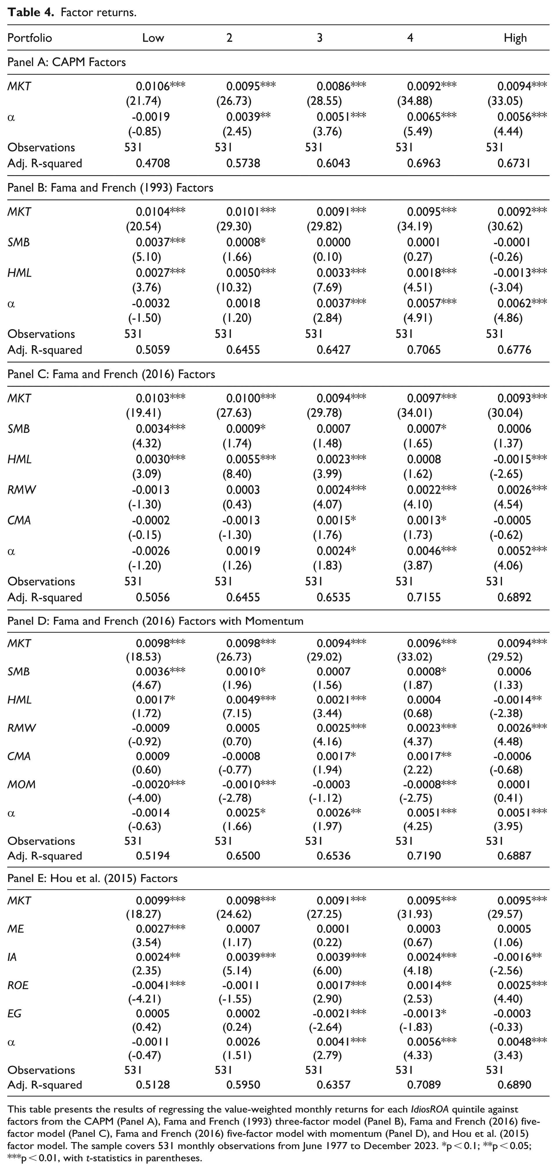
We then conduct regressions using our portfolio returns as the dependent variable and factors of other commonly employed asset pricing models as independent variables, specifically the capital asset pricing model (Panel A), the Fama and French (1993) three-factor model (Panel B), the Fama and French (2016) five-factor model (Panel C), the Fama and French (2016) five-factor model including momentum (Panel D), and the Hou et al. (2015) factors.¹³ We present our results in Table 4.

From Table 4, we make two conclusions. First, there appear to be no consistent factors that are significantly correlated with the portfolio returns from our models that would indicate that our formation based on the signed value of idiosyncratic profitability is systematically associated with one of the factors within these models considered. From Panel B, there is some evidence that there is a negative correlation as we move from the low to high portfolio with the HML factor in the Fama and French (1993) three-factor model, consistent with the results in Novy-Marx (2013). However, this result is not consistently replicated across the Fama and French (2016) factors with and without momentum.

When our portfolio returns are regressed against the Hou et al. (2015) factors, there is an increasing pattern in the profitability (ROE) factor and a decreasing pattern in the investment (IA) factor, though this is not monotonic when moving from the low to high IdiosROA portfolios. While idiosyncratic profitability will be associated with total profitability, such as ROE, we are still able to generate significant alphas in portfolios 3, 4 and High. This is also consistent with Table 4 in our Online Appendix, where we document that the IdiosROA factor is still statistically significant while controlling for the six most closely related anomalies (Operating profitability RD, Cash-based operating profitability, net income / book equity, ROA (quarterly), gross profits / total assets, and efficient frontier index). This includes achieving an alpha of 0.47% per month (t-statistic 2.55) while controlling for all six simultaneously in a Fama and French six-factor model (see Online Appendix Table 5).

The second conclusion we draw is that there are still positive hedge portfolio returns in the alphas when regressing portfolio returns against the factors from these models. Abnormal returns of the idiosyncratic portfolio return spread (high quintile alpha minus low quintile alpha) relative to the CAPM is 0.75% per month. This is repeated with abnormal returns of 0.94% per month for the Fama and French (1993) model, 0.78% for the Fama and French (2016) model, 0.65% per month for the Fama and French (2016) model including momentum, and 0.59% per month for the Hou et al. (2015) model. The results are larger than the baseline when our analysis is limited to only the month of portfolio formation itself, ranging from 0.77% per month for the Fama and French (2016) five-factor model with momentum to 1.31% per month for the Fama and French (1993) three-factor model. This result demonstrates that the hedge portfolio returns based on idiosyncratic profitability is additional to these known risk factors and is at least comparable to the 0.52% monthly abnormal return on gross profitability relative to the Fama and French (1993) three-factor model as documented by Novy-Marx (2013).

To consider the robustness of our analysis, we include an Online Appendix utilizing the online report generator from Mihail Velikov.¹⁴ Overall, the results from this report indicate that the use of IdioROA as a signal adds to the “factor zoo.” Specifically, the IdiosROA strategy’s gross (net) Sharpe ratio of 0.46 (0.36) is greater than 88% (93%) of the 212 documented anomaly Sharpe ratios (see Online Appendix, Figure 2). Further, after accounting for trading costs, the trading strategy based on idiosyncratic profitability generates a positive net generalized alpha for all of the CAPM and Fama and French three-, four-, five-, and six-factor models. In these cases, IdiosROA ranks between the 95^th and 99^th percentiles in terms of how much it could have expanded the achievable investment frontier relative to the other 212 anomalies.

4.3. Idiosyncratic profitability quintiles

We provide further details of the idiosyncratic profitability quintile in Table 5. First, in Panel A, we provide the persistence of firms’ occurrence in each quintile. Specifically, we calculate the percentage of firms that are reported in each IdiosROA quintile in quarter t + 1 against their occurrence in quarter t. Of note is that there is a large persistence in the quintiles in adjacent quarters, ranging from 53.19% of firms remaining in quintile 4% to 71.16% in the highest quintile. We also note that there is a non-trivial portion of firms that move up and down a quintile from quarter t to quarter t + 1. Further, there are instances where firms jump between the quintiles, with 3.98% (4.03%) moving from the lowest to the highest (highest to lowest) quintile in adjacent quarters.

Table 5.

Properties of IdiosROA quintiles.

Panel A: Persistence of IdiosROA Quintile
		quarter t + 1
		Low	2	3	4	High
quarter t	Low	65.87	17.14	6.59	6.42	3.98
	2	14.88	56.47	18.81	7.30	2.55
	3	6.00	18.56	56.49	15.59	3.37
	4	5.92	7.62	16.25	53.19	17.02
	High	4.03	2.71	3.67	18.43	71.16
Panel B: IdiosROA Quintile Descriptives
	IdiosROA Quintile
	Low	2	3	4	High	High–Low
IOR	0.387	0.373	0.383	0.450	0.479	0.092(38.10)***
Coverage	3.319	3.476	3.572	4.330	5.142	1.823(41.84)***
Size	6.384	7.473	7.471	7.011	6.402	0.019(1.24)
Spread	0.160	0.229	0.024	0.192	0.200	0.041(18.33)***

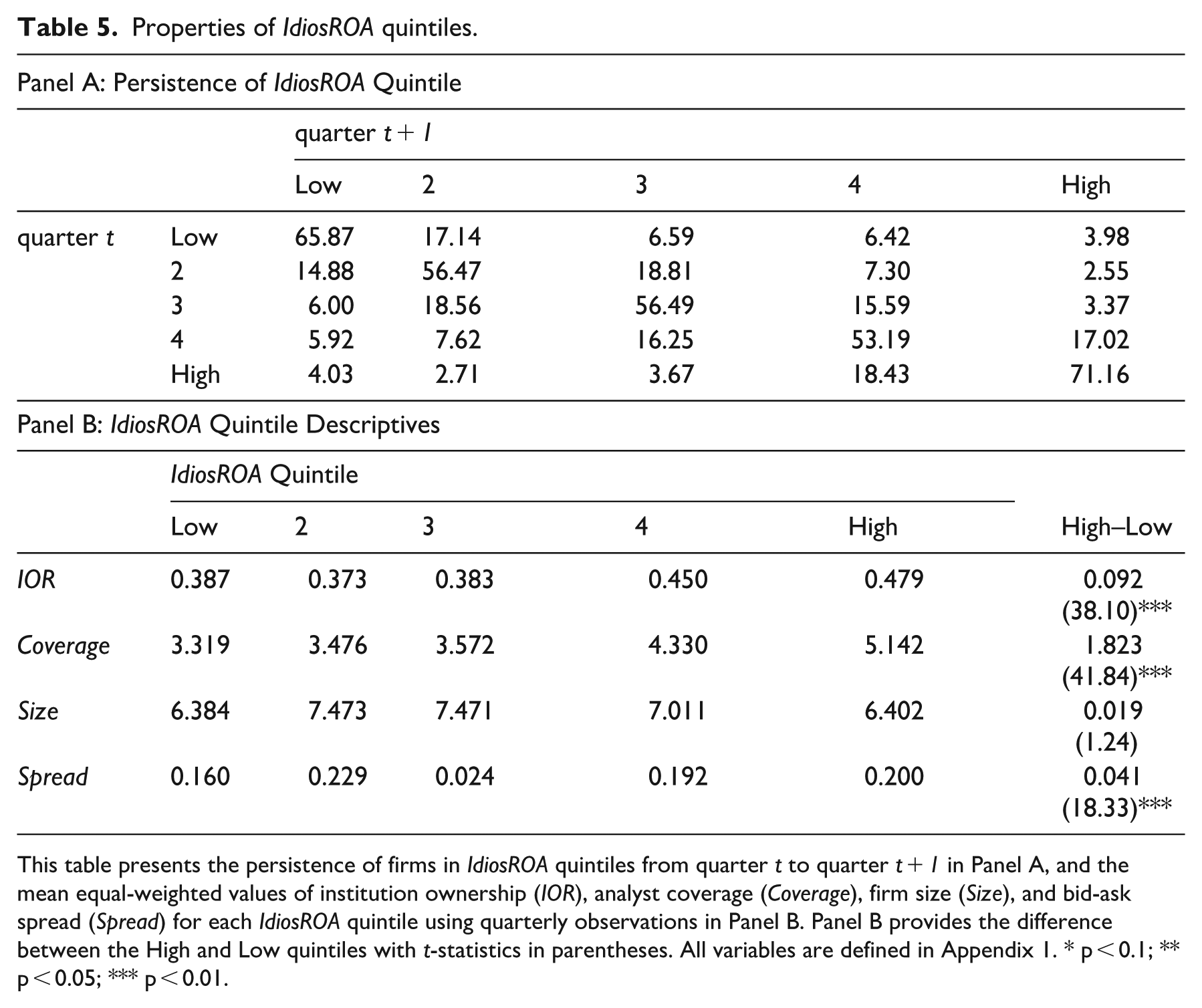
This table presents the persistence of firms in IdiosROA quintiles from quarter t to quarter t + 1 in Panel A, and the mean equal-weighted values of institution ownership (IOR), analyst coverage (Coverage), firm size (Size), and bid-ask spread (Spread) for each IdiosROA quintile using quarterly observations in Panel B. Panel B provides the difference between the High and Low quintiles with t-statistics in parentheses. All variables are defined in Appendix 1. * p < 0.1; ** p < 0.05; *** p < 0.01.

We next explore whether the sophistication of investors appears to be related to investment into specific idiosyncratic profitability quintiles, with the results presented in Panel B of Table 5. Under the assumption that institutional investors are sophisticated investors, we would expect that they would hold a greater proportion of stock in firms with higher IdiosROA. We take the proportion of institutional ownership held (IOR) as defined in Appendix 1 at the end of each fiscal quarter. Due to data limitations, our sample is restricted to a period beginning in 1980. We find that the proportion of institutional holdings is fairly monotonically increasing across the quintiles of IdiosROA from 38.7% in the lowest to 47.9% in the highest quintile, with the difference being statistically significant (9.2%, t-stat 38.10). This result is consistent with Oehmichen et al. (2021), who show that dedicated institution investors exert effort to understand a firm’s unique strategy and help reduce the pressure faced by management in implementing such a strategy.

Similarly, we find that there is a monotonic increase in mean analyst following (Coverage) across the quintiles from 3.319 in the lowest to 5.142 in the highest, with the difference (1.823, t-stat 41.84) being highly statistically significant. The significant increases in institutional investor ownership and analyst coverage, however, do not appear to be related to firm size, with no difference across the low and high idiosyncratic profitability quintiles based on Size. Likewise, bid-ask spread (Spread), while demonstrating a significant difference between the high and low quintiles (0.041, t-stat 18.33), is not monotonic in any manner, with the highest (lowest) mean spread in the second (Low) quintile.

Overall, our results are consistent with the notion that sophisticated investors are more likely to understand the idiosyncratic component of profitability and will have a higher proportion of holdings in higher quintiles of IdiosROA.

4.4. Market and industry profitability

Finally, we consider whether predictable abnormal returns could be generated from a hedge portfolio trading strategy based on either the market (MktROA) or industry (IndROA) components of profitability. We report our results in Table 6.

Table 6.

Monthly returns on market and industry profitability quintiles.

	MktROA		IndROA
	VWRet	EWRet	VWRet	EWRet
Low	0.0110	0.0120	0.0077	0.0107
2	0.0095	0.0114	0.0135	0.0125
3	0.0115	0.0121	0.0111	0.0117
4	0.0126	0.0129	0.0124	0.0128
High	0.0105	0.0121	0.0118	0.0127
High–Low	-0.0005(-0.26)	0.0001(0.11)	0.0041(1.81)*	0.0020(1.66)*
N	531	531	531	531

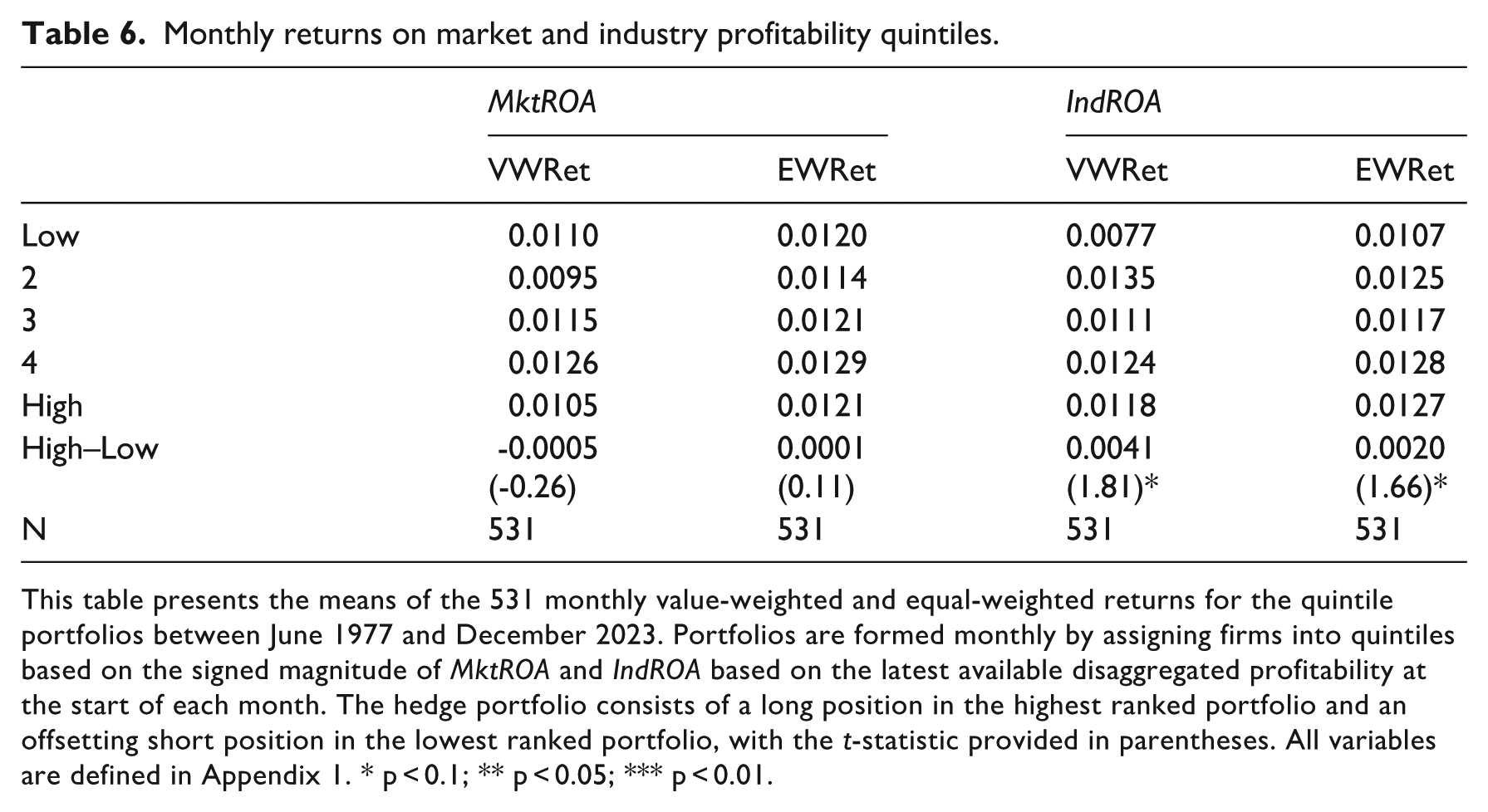
This table presents the means of the 531 monthly value-weighted and equal-weighted returns for the quintile portfolios between June 1977 and December 2023. Portfolios are formed monthly by assigning firms into quintiles based on the signed magnitude of MktROA and IndROA based on the latest available disaggregated profitability at the start of each month. The hedge portfolio consists of a long position in the highest ranked portfolio and an offsetting short position in the lowest ranked portfolio, with the t-statistic provided in parentheses. All variables are defined in Appendix 1. * p < 0.1; ** p < 0.05; *** p < 0.01.

In the first set of columns, we repeat our main analysis but sort firms into quintiles based on the signed value of MktROA and determine the value-weighted and equal-weighted returns on these portfolios. Across 531 monthly means, we find no statistical difference in the High–Low returns. We then repeat our analysis, placing firms in quintiles based on the signed value of IndROA. Here we find a statistical hedge portfolio return of 0.41% per month using value-weighted returns and 0.20% per month using equal-weighted returns. The t-stats of 1.81 and 1.61, respectively, however, would indicate that these are not statistically meaningful. Overall, this indicates that the fundamental approach used to identify the idiosyncratic portion of a firm’s earnings, which can be related to the successful outcome of a firm’s strategy response to market and industry pressures, is a meaningful approach to form an investing portfolio.

5. Conclusion

Using the profitability disaggregation model in Jackson et al. (2018), we investigate whether a trading strategy based on idiosyncratic profitability is able to generate predictable abnormal returns. We interpret the firm-idiosyncratic profitability component as the outcome of a firm’s strategic responses to competitive pressures from market and industry sources. Our results indicate that the average hedge portfolio value-weighted returns taking a long (short) position in firms with high (low) idiosyncratic profitability is 0.66% per month. After controlling for popular asset pricing models, we still generate significant abnormal returns. Overall, we conclude that this trading strategy is able to generate predictable abnormal returns, and this idiosyncratic profitability signal adds to the “factor zoo.”

Our study makes several contributions to the literature. First, we demonstrate that predictable abnormal returns can be generated using a trading strategy based on ranking firms according to the level of their idiosyncratic profitability. We document significant hedge portfolio returns by trading on an economically meaningful component of a firm’s profitability, that is its profitability capturing the outcome of the implementation of the firm strategy. Our approach differs from anomalies popularized by Novy-Marx (2013) and Hou et al. (2015) by interpreting the firm’s idiosyncratic profitability as representing the outcome of a firm’s strategic response to the competitive pressures within the industry and general macroeconomic conditions. Second, prior research focuses on the industry-specific and idiosyncratic components of profitability, assuming that the industry component for all firms will be the average earnings within the industry-quarter, with the idiosyncratic component being the remainder. Our approach explicitly models a firm’s profitability to be comprised of market-wide, industry-specific, and idiosyncratic profitability, allowing for cross-sectional variation in the components by allowing for historical sensitivities of a firm’s profitability to the market and industry, thus better capturing the idiosyncratic component. By more accurately capturing the idiosyncratic component of a firm’s profitability, we document significant hedge portfolio returns by trading on an economically meaningful component of a firm’s profitability, that is its profitability capturing the outcome of the implementation of firm strategy, as opposed to a statistical observation. In addition, our study enhances our understanding of stock return predictability, which is a fundamental topic in financial economics (Dong et al., 2022). Our results provide valuable insights into the interplay between profitability components and investor behavior, enriching the discourse of financial economics.

Finally, this study has implications for future research. First, our results highlight the usefulness of earnings disaggregation for enhancing our understanding of the way that markets interpret aggregate accounting information, and especially for providing insights into well-accepted beliefs in the literature. For example, prior studies show that accounting for idiosyncratic earnings is able to further understand the role of bias in reported earnings (Jackson et al., 2017), improve future performance forecasts (Jackson et al., 2018), pinpoint the source of conservatism in accounting (Jackson et al., 2025), and explain the use of relative performance evaluation in compensation contracts (Dikolli et al., 2025).

Second, our findings suggest that further research is warranted into the role of idiosyncratic earnings in asset pricing. As we highlighted earlier, idiosyncratic profitability and idiosyncratic risk are distinct constructs that measure different underlying economic ideas. However, to the extent that both idiosyncratic profitability and idiosyncratic risk capture components unexplained by market and industry factors, if idiosyncratic profitability predicts idiosyncratic risk, it challenges purely systematic asset-pricing frameworks and will help refine multifactor models and forecasting of volatility.

Key theoretical and practical contributions

Theoretical

1. The study demonstrates that the firm-idiosyncratic component of profitability, interpreted as the outcome of firm strategy, is systematically priced and generates abnormal returns beyond standard asset-pricing factors.

Methodological

2. By refining profitability disaggregation using firm-specific earnings betas, the paper provides a more accurate way to isolate the strategy-driving portion of profitability, thus improving our understanding of which earnings components drive return predictability.

Practical

3. The finding that idiosyncratic profitability produces abnormal returns provides investors with a robust trading signal and insights into how markets underreact to strategy-driven performance.

Supplemental Material

sj-pdf-1-aum-10.1177_03128962261425895 – Supplemental material for Excess returns on idiosyncratic profitability: Evidence from a hedge portfolio strategy

Supplemental material, sj-pdf-1-aum-10.1177_03128962261425895 for Excess returns on idiosyncratic profitability: Evidence from a hedge portfolio strategy by Miaodi Han, Andrew B Jackson and Gary S Monroe in Australian Journal of Management

Footnotes

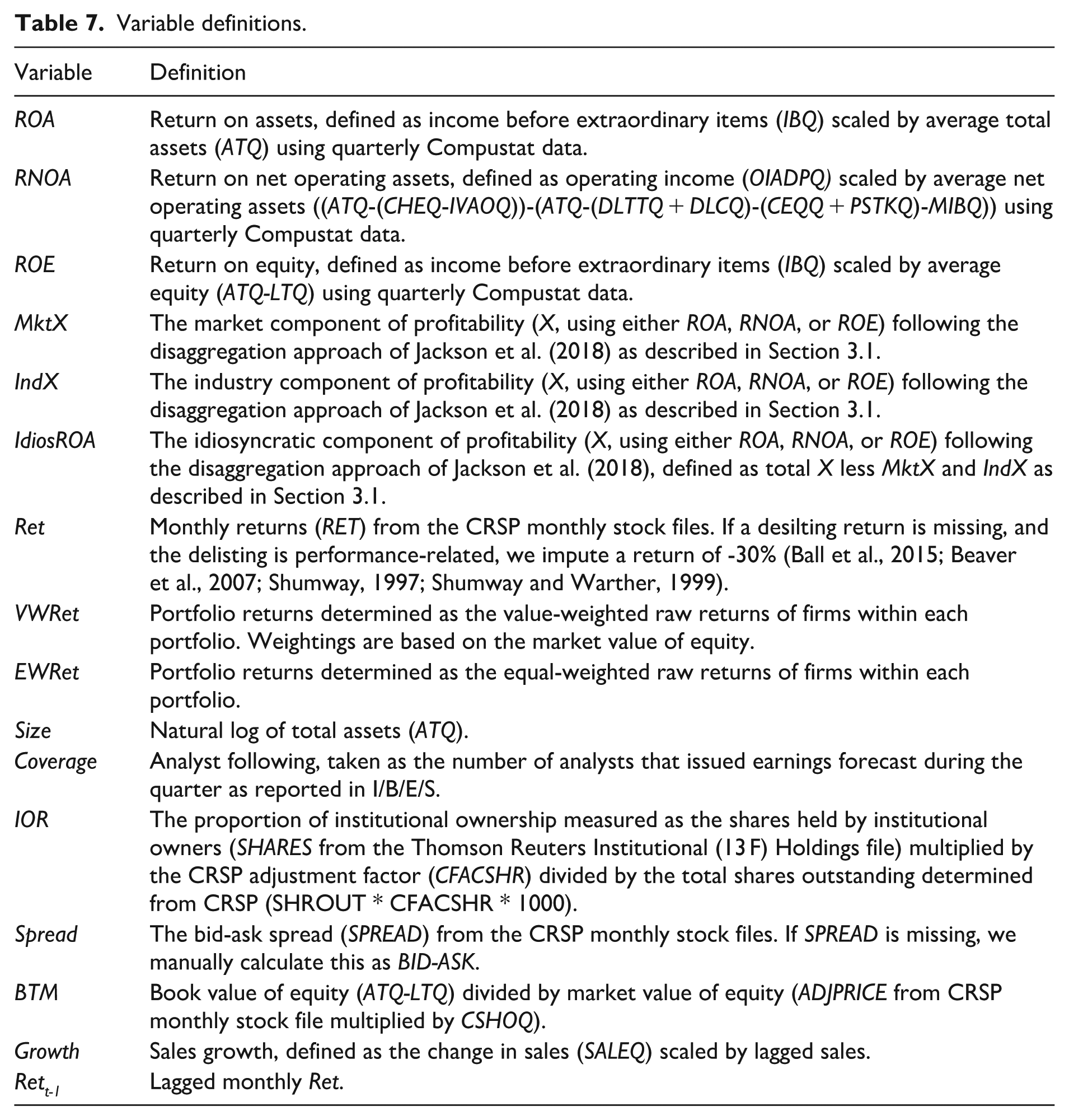
Appendix 1

Table 7.

Variable definitions.

Variable	Definition
ROA	Return on assets, defined as income before extraordinary items (IBQ) scaled by average total assets (ATQ) using quarterly Compustat data.
RNOA	Return on net operating assets, defined as operating income (OIADPQ) scaled by average net operating assets ((ATQ-(CHEQ-IVAOQ))-(ATQ-(DLTTQ + DLCQ)-(CEQQ + PSTKQ)-MIBQ)) using quarterly Compustat data.
ROE	Return on equity, defined as income before extraordinary items (IBQ) scaled by average equity (ATQ-LTQ) using quarterly Compustat data.
MktX	The market component of profitability (X, using either ROA, RNOA, or ROE) following the disaggregation approach of Jackson et al. (2018) as described in Section 3.1.
IndX	The industry component of profitability (X, using either ROA, RNOA, or ROE) following the disaggregation approach of Jackson et al. (2018) as described in Section 3.1.
IdiosROA	The idiosyncratic component of profitability (X, using either ROA, RNOA, or ROE) following the disaggregation approach of Jackson et al. (2018), defined as total X less MktX and IndX as described in Section 3.1.
Ret	Monthly returns (RET) from the CRSP monthly stock files. If a desilting return is missing, and the delisting is performance-related, we impute a return of -30% (Ball et al., 2015; Beaver et al., 2007; Shumway, 1997; Shumway and Warther, 1999).
VWRet	Portfolio returns determined as the value-weighted raw returns of firms within each portfolio. Weightings are based on the market value of equity.
EWRet	Portfolio returns determined as the equal-weighted raw returns of firms within each portfolio.
Size	Natural log of total assets (ATQ).
Coverage	Analyst following, taken as the number of analysts that issued earnings forecast during the quarter as reported in I/B/E/S.
IOR	The proportion of institutional ownership measured as the shares held by institutional owners (SHARES from the Thomson Reuters Institutional (13 F) Holdings file) multiplied by the CRSP adjustment factor (CFACSHR) divided by the total shares outstanding determined from CRSP (SHROUT * CFACSHR * 1000).
Spread	The bid-ask spread (SPREAD) from the CRSP monthly stock files. If SPREAD is missing, we manually calculate this as BID-ASK.
BTM	Book value of equity (ATQ-LTQ) divided by market value of equity (ADJPRICE from CRSP monthly stock file multiplied by CSHOQ).
Growth	Sales growth, defined as the change in sales (SALEQ) scaled by lagged sales.
Ret_t-1	Lagged monthly Ret.

Acknowledgements

We appreciate comments from two anonymous reviewers, John Campbell, Jeff Coulton, Jesper Haga, Wayne Landsman, Kevin Li, Chelsa Liu (editor), John Lyon, Vic Naiker, Ryan Peng, Brian Rountree, Naomi Soderstrom, Mark Wilson, Teri Yohn, and seminar participants at Shanghai Lixin University of Accounting and Finance, University of Melbourne, UNSW Sydney, University of Queensland, University of Technology Sydney, and the 2019 AFAANZ Annual Conference. All errors remain our own responsibility.

Final transcript accepted on 12 December 2025 by Chelsea Liu (Deputy Editor).

Funding

The authors disclosed receipt of the following financial support for the research, authorship, and/or publication of this article: Andrew Jackson acknowledges funding from a UNSW Scientia Fellowship and the Australian Research Council’s Discovery Projects funding scheme (project number DP210101354).

ORCID iDs

Miaodi Han

Andrew B Jackson

Supplemental material

Supplemental material for this article is available online.

Notes

References

Albuquerque

(2009) Peer firms in relative performance evaluation. Journal of Accounting and Economics 48: 69–89.

Ayers

Freeman

(1997) Market assessment of industry and firm earnings information. Journal of Accounting and Economics 24: 205–218.

Ball

Gerakos

Linnainmaa

, et al. (2015) Deflating profitability. Journal of Financial Economics 117: 225–248.

Beaver

McNichols

Price

(2007) Delisting returns and their effect on accounting-based market anomalies. Journal of Accounting and Economics 43: 341–368.

Beaver

Kettler

Scholes

(1970) The association between market determined and accounting determined risk measures. The Accounting Review 45: 654–682.

Bernard

Thomas

(1990) Evidence that stock prices do not fully reflect the implications of current earnings for future earnings. Journal of Accounting and Economics 13: 305–340.

Bhojraj

Lee

CMC

Oler

(2003) What’s my line? A comparison of industry classification schemes for capital market research. Journal of Accounting Research 41: 745–774.

Bouchaud

J-P

Kruger

Landier

, et al. (2019) Sticky expectations and the profitability anomaly. Journal of Finance 74: 639–674.

Brown

Ball

(1967) Some preliminary findings on the association between the earnings of a firm, its industry, and the economy. Journal of Accounting Research 5: 55–77.

10.

Dikolli

Jackson

Plumlee

(2025) Relative Performance Evaluation in Accounting-based CEO Bonus Contracts: Evidence from Profitability Components (Working Paper). Charlottesville, VA: University of Virginia.

11.

Dong

Rapach

, et al. (2022) Anomalies and the expected market return. Journal of Finance 77: 639–681.

12.

Durnev

Morck

Yeung

(2004) Value-enhancing capital budgeting and firm-specific stock return variation. Journal of Finance 59: 65–105.

13.

Fama

French

(1993) Common risk factors in the returns on stocks and bonds. Journal of Financial Economics 33: 3–56.

14.

Fama

French

(2016) Dissecting anomalies with a five-factor model. The Review of Financial Studies 29: 69–103.

15.

Gopalan

Milbourn

Song

(2010) Strategic flexibility and the optimality of pay for sector performance. The Review of Financial Studies 23: 2060–2098.

16.

Harvey

Liu

Zhu

(2016) . . . and the cross-section of expected returns. The Review of Financial Studies 29: 5–68.

17.

Hou

Xue

Zhang

(2015) Digesting anomalies: An investment approach. The Review of Financial Studies 28: 650–705.

18.

Hui

Yeung

(2013) Underreaction to industry-wide earnings and the post-forecast revision drift. Journal of Accounting Research 51: 701–737.

19.

Hui

Nelson

Yeung

(2016) On the persistence and pricing of industry-wide and firm-specific earnings, cash flows, and accruals. Journal of Accounting and Economics 61: 185–202.

20.

Jackson

Rountree

Sivaramakrishnan

(2017) Earnings co-movements and earnings manipulation. The Review of Financial Studies 22: 1340–1365.

21.

Jackson

Morris

(2020) Earnings co-movements and the informativeness of earnings. ABACUS 56: 295–319.

22.

Jackson

Plumlee

Rountree

(2018) Decomposing the market, industry, and firm components of profitability: Implications for forecasts of profitability. The Review of Financial Studies 23: 1071–1095.

23.

Jackson

Shan

Taylor

(2025) Asymmetric timeliness in earnings: Insights from earnings decomposition (Working Paper). Sydney, NSW: UNSW Sydney.

24.

Jegadeesh

Titman

(1993) Returns to buying winners and selling losers: Implications for stock market efficiency. Journal of Finance 48: 65–91.

25.

Lakonishok

Shleifer

Vishny

(1994) Contrarian investment, extrapolation, and risk. Journal of Finance 49: 1541–1578.

26.

Landsman

Miller

Peasnell

, et al. (2011) Do investors understand really dirty surplus? The Accounting Review 86: 237–258.

27.

Litov

Moreton

Zenger

(2012) Corporate strategy, analyst coverage, and the uniqueness paradox. Management Science 58: 1797–1815.

28.

Mueller

(1977) The persistence of profits above the norm. Economica 44: 369–80.

29.

(2020) CEO’s outside opportunities and relative performance evaluation: Evidence from a natural experiment. Journal of Financial Economics 137: 679–700.

30.

Novy-Marx

(2013) The other side of value: The gross profitability premium. Journal of Financial Economics 108: 1–28.

31.

Novy-Marx

Velikov

(2024) Assaying Anomalies (Working Paper). Rochester, NY: University of Rochester.

32.

Oehmichen

Firk

Woldd

, et al. (2021) Standing out from the crowd: Dedicated institutional investors and strategy uniqueness. Strategic Management Journal 42: 1083–1108.

33.

Shiller

Fischer

Friedman

(1984) Stock prices and social dynamics. Brookings Papers on Economic Activity 2: 457–510.

34.

Shumway

(1997) The delisting bias in CRSP data. Journal of Finance 52: 327–340.

35.

Shumway

Warther

(1999) The delisting bias in CRSP’s Nasdaq data and its implications for the size effect. Journal of Finance 54: 2361–2379.

36.

Sloan

(1996) Do stock prices fully reflect information in accruals and cash flows about future earnings? The Accounting Review 71: 289–315.

37.

Tice

(2024) The role of common risk in the effectiveness of explicit relative performance evaluation. Management Science 70: 1635–1655.

38.

Veldkamp

(2006) Media frenzies in markets for financial information. American Economic Review 96: 577–601.

39.

Vorst

Yohn

(2018) Life cycle models and forecasting growth and profitability. The Accounting Review 93: 357–381.

40.

Waring

(1996) Industry differences in the persistence of firm-specific returns. American Economic Review 86: 1253–1265.