Tests of asset pricing models in Australia using non-normal distributions

Abstract

This article demonstrates that Australian equity returns and factors are strongly non-normal and that non-normality seems to be adequately modelled as a jointly multivariate t random variable with 7 degrees of freedom. When means and alphas are estimated using maximum likelihood estimation under the multivariate t case, we find dramatic changes in the estimates of the mean of the test assets, and find that the sign of the price of SMB risk flips from positive to negative (though insignificant). The evidence against asset pricing models is larger when returns are non-normal. This methodology can be viewed as a robust estimator, and its results suggest caution should be applied in interpreting estimates of risk premia and alphas obtained using non-robust methods.

JEL Classification: G1, C1

1. Introduction

Over the past several decades, our understanding of the cross-sectional behaviour of equity returns has improved markedly. Research has shown that exposure to risk factors, including size, value, asset growth, and profitability are cross-sectionally related to expected returns. At the same time, evidence that stock returns do not follow a normal distribution has grown (see, among many others, Fama (1965), Affleck-Graves and McDonald (1989), and Richardson and Smith (1993)). Despite this evidence, the vast majority of tests of asset pricing models either assume multivariate normality explicitly or base their inference on sample average returns, which is the maximum likelihood estimator of means if returns are normal, or ordinary least squares estimates, which are also consistent with maximum likelihood under normality. Of course, standard errors and critical values of test statistics can be constructed accounting for non-normality. However, if returns are not normally distributed, then sample averages are not statistically efficient as an estimate of the mean since it is not the maximum likelihood estimator, which, according to the Rao-Blackwell theorem, is asymptotically efficient. Indeed, the current literature (e.g. MacKinlay and Richardson, 1991 and Zhou, 1993) shows that tests based on normality, including the seemingly ubiquitous Gibbons-Ross-Shanken test (Gibbons et al., 1989), are biased towards over-rejection when returns are fat-tailed. However, there has been little work that explicitly accounts for the non-normality of returns by estimating factor model alphas under alternative return distributional assumptions, which we now do using Australian equity returns.

The recent Australian asset pricing research has focused on the Fama and French (1993, 2015) asset pricing models, and the literature is a little mixed in how relevant factors other than the market return are in pricing Australian stock returns. Halliwell et al. (1999) find that the HML factor marginally improves the performance of asset pricing models in Australia over the CAPM. Gaunt (2004) finds that the three-factor model of Fama and French (1993) improves pricing over the CAPM, but much of the heavy lifting is done by SMB, the size factor, not the value factor HML. Brailsford et al. (2011) use a portfolio formation strategy as in Brailsford et al. (2012) that acknowledges the significant differences between the Australian and US equity markets and tweaks the traditional definition of the size portfolios, and they find that size and value factors are significant and priced in the cross-section and improve asset pricing over the single-factor CAPM. Chiah et al. (2016) and Huynh (2018) consider the five-factor model of Fama and French (2015) and find that the profitability and asset growth factors are significant and provide an improvement over the basic three-factor model. In particular Huynh (2018) compares how the 3 factor and 5 factor Fama-French models perform in explaining a set of 16 anomalies previously documented in the Australian market, finding that the five-factor model does a much better job at rendering alphas statistically indistinguishable from zero at a range of significance level, and he shows that the absolute value of alpha decreases for 15 out of the 16 anomalies when using the five-factor model as opposed to the one-factor model. Gharghori et al. (2007) find that default risk is not priced in Australia, and the Fama-French factors aren’t proxying for default risk. Durand et al. (2016) reject a four-factor model that includes momentum. ¹ Chai et al. (2013) find that while liquidity explains some variability in returns above the standard three-factor model plus momentum, its contribution to explanatory power is marginal.

Much of the Australian literature has focused on estimates of asset pricing models using ordinary least squares, which is consistent with maximum likelihood when residuals are normally distributed. However, it is well known that equity returns, including in Australia, exhibit nonnormality, including more frequent tail returns that generate leptokurtosis. There is a large literature on non-normality in portfolio returns, including Richardson and Smith (1993), Zhou (1993), Tu and Zhou (2004), and Kan and Zhou (2017). There are a number of ways to deal with the non-normality. One approach is to conduct inference using OLS estimates that account for the non-normality of returns, including using GMM or constructing test statistics that explicitly adjust the standard errors of the alphas for non-normality. Examples of this second approach are MacKinlay and Richardson (1991), who construct a GMM-based Wald test of the zero alpha restriction, including an explicit example where returns are multivariate t. The test continues to use the OLS estimates of the alphas, which we have seen from Zhou (1993) and Kan and Zhou (2017), are inefficient when the data is not multivariate t.

Zhou (1993) shows how to adjust critical values for the Wald-type tests, accounting for non-normal elliptical residuals that account for uncertainty in the distribution of the factor realizations. He finds that after accounting for plausible distributions, the CAPM can no longer be rejected in some cases in which inference based on the normality assumption rejects the efficiency of the market return. Finally, Kan and Zhou (2017) present an alternative approach that directly estimates factor model parameters using maximum likelihood that accounts for the non-normality of returns and factors and constructs a likelihood ratio test for asset pricing models.

Given the strong evidence of non-normality and the peculiarities of asset pricing models in Australia, it seems useful to assess the extent to which results depend on the use of inefficient statistical methods. This article conducts an empirical analysis of the multivariate t distribution in Australian equity returns and explore the impact of testing the five-factor asset pricing model of Fama and French (2015) on Australian returns, accounting for leptokurtosis in returns using the multivariate t distribution. The student t distribution has been in favour for quite some time. For example, more than 50 years ago, Praetz (1972) and Blattberg and Gonedes (1974) suggested it, and it has a wide history in applications to modelling financial returns, including in GARCH models by Bollerslev (1987). In this article, we follow Kan and Zhou (2017) and consider the multivariate t distribution to model the joint distribution of returns and factors. Maximum likelihood estimates of complex models of large-scale distributions is, in general, not a trivial exercise. In the case of the multivariate normal distribution, the sample mean and covariance matrix are the maximum likelihood estimates. The multivariate t distribution is only marginally more complex, given the expectation-maximization algorithm of Dempster et al. (1977) with a particular application by Liu and Rubin (1995).

We find that the use of OLS as opposed to the more efficient multivariate t-based maximum likelihood has a massive impact on returns. We find that the size effect, which is somewhat marginal even under the assumption of normality, with a point estimate of 19 basis points per month, which is about 1 standard error from zero; yet when the price of SMB risk is estimated using the non-normality assumption, it flips sign and is about −11 basis points per month. The size of the market risk premium also drops slightly. The estimates of the means and alphas of the test assets also change markedly when non-normality is accounted for, with the largest changes occurring, perhaps unsurprisingly, among small-cap and growth stocks. Interestingly, estimates of the standard deviation of returns and their betas are much less dependent on distribution assumptions than means and alphas. We also find that the three- and five-factor models are unable to be rejected by a likelihood ratio test applied to 16 size and book-to-market sorted portfolios if returns are assumed to be normally distributed (though they are rejected when we form test assets by sorting on size and asset growth and size and profitability) but we do reject all asset pricing models when we allow returns to come from a multivariate t distribution.

We find marked differences in conclusions about the five-factor pricing model in Australia when we allow returns to be multivariate Student t rather than normal. We find that the size effect flips sign from positive to negative. Since most Australian asset pricing tests typically find a robust size effect, this result is surprising; but it is not without precedent in Australia. Faff (2001) constructs novel proxies for the size and value factors using ‘off-the-shelf’ style returns and finds a negative premium on the size factor, in contrast to US results, in which size is remarkably robust. Indeed, using a novel approach to testing the explanatory power of asset pricing models using a firm-level bootstrap-based analysis, Harvey and Liu (2021) find that only the market return and the size factor (SMB) are priced in US returns. Hoang et al. (2019) show, using the same methodology in Australian equity returns, that only the market return is reliably concluded as providing valid pricing of returns when the problem of data mining is accounted for. We also find that the evidence against asset pricing models is generally stronger when we use multivariate t returns. Given the marked differences between the estimated risk premia under the standard and robust estimation methods and the dramatic loss of efficiency in standard sample estimates, these results have implications for investors, regulators and portfolio managers.

The remainder of the article proceeds as follows. Section 2 presents a discussion of the data we use. Section 3 presents empirical tests of non-normality in the portfolio and factor returns. The estimation methodology that we use is described in Section 4. The empirical results are presented in Section 5, some robustness and simulation results are presented in Section 7, and we conclude in Section 8.

2. Data

To construct portfolio returns for Australian stocks, we use stock and accounting data sourced from the Securities in Research Centre Asia-Pacific (SIRCA), as it has the widest coverage for historical Australian equity returns. A significant problem with Australian equity returns is non-trading, which occurs because of the very large number of extraordinarily small stocks. To address this, we apply a number of filters. To illustrate the magnitude of the problem, before any screening of the data 11.15% of monthly return observations represent months where a return could not be recorded due to non-trading (either the current or previous month's price record is missing). This decreases to 6.45% and 3.39% when focusing on the top 1000 and 500 firms by market capitalization, respectively. And because we are constructing portfolio and factor returns by sorting stocks based on accounting data, we have to drop stocks that don’t have accounting data, and larger, more liquid stocks are far more likely to have accounting data. Accounting data is sourced from company annual reports from the SIRCA fundamental files. This data extracts over 600 individual items from the financial reports of Australian firms.

The final sample includes only ordinary stocks (Share Code ‘01’) of non-financial firms that are listed on the Australian Stock Exchange. Returns are calculated using SIRCA’s price relative series, which adjusts returns for dividends and capital adjustments such as stock splits. When a stock doesn’t trade in the present or previous month, a price-relative isn’t available, and we treat the returns as missing. When a return of over 300% is observed, that reverses the following month, both months’ returns are treated as an error and set to missing. There were only 24 pairs of monthly observations that were revised from this procedure. Although we only keep stocks with an ordinary share code of ‘01’, we also search for and exclude any firms whose company name includes the words ‘Fund’ or ‘ETF’. There are roughly 5000 monthly observations that are removed. In line with previous studies, and to ensure a fair comparison, we only keep stocks that have all of the following accounting variables: BM (Shareholders Equity), MBM (requires Operating Expenses), AG (total assets), profitability (NPBT) and market capitalization. Firms must therefore be at least 2 years old as AG requires 2 years of accounting data to calculate.

Stock and accounting data are available from July of 1984; however, the number of firms with coverage in these early years is rather low. We thus restrict our attention to returns starting January 1991 onwards. Our final sample contains 2794 unique firms over the period January 1991 to December 2023, with a total of 395,694 firm-month observations combining valid monthly stock and annual accounting data.

2.1. Test assets

Brailsford et al. (2012) argue quite convincingly that the Australian market has some peculiarities compared with the US markets. The quintile of the largest stocks in Australia accounts for 95% of the total market capitalization of all stocks. The smallest 60% of stocks is only 1.6% of the total market capitalization. In the United States, the largest size quintile accounts for about 75% of the total market capitalization and the smallest 60% of stocks account for 13% of the total market capitalization. In light of this, they suggest defining large stocks as the top 50 stocks by market cap, the second portfolio as stocks ranked 51–200. The number 200 is chosen to correspond to the number of stocks in the ASX200 index, which is the main index used in the Australian market. The third portfolio is the next 100. The fourth portfolio contains stocks ranked 301–500. The fifth is everything after that.

The procedure for forming test assets following Fama and French (1992) involves forming portfolios based on independent sorts on size and some other characteristic, and then allocating stocks based on those independently formed breakpoints.

Inspired by this approach, we construct portfolios by sorting stocks into four portfolios every year. The smallest 50% of stocks are small, the second smallest portfolio consists of all stocks between the 50th and 75th percentile. The second largest portfolio stocks are those stocks between the 75th and 90th percentile by market cap. The largest portfolios are the largest 10% of stocks. We then form portfolios by sorting on characteristics like value, profitability and asset growth by sorting within these bins. By using dependent sorts, we avoid problems that arise with zero stocks in some months in some portfolios when using two-dimensional independent sorts. The Australian market has significantly fewer stocks than the US data typically studied, so using independent two-way sorts finds many fewer stocks in some portfolios. In several cases, we find that some of our portfolios have zero stocks in them if we sort independently. If we do independent sorts and define the largest stock portfolio as the top 10% of firms by market cap, then in all three bivariate sorts, there are many portfolios with either zero or one stock. And significant heterogeneity in the number of stocks in portfolios results in significant variation in the amount of diversification across portfolios, which in turn results in dramatic variation in variance across portfolios. On the other hand, running independent sorts facilitates cross-portfolio comparison – if the sorts are independent, a small-value stock might will be markedly different from a large-value stock. So caution must be exercised in comparing portfolio returns from the non-size characteristics.

Ranking is done at the end of the calendar year to allow six months to elapse to ensure all annual reports released during the June-ending Australian financial year are publicly available. The typical US reporting cycle ends in December, and the United States studies use a June 30 ranking date. Because the Australian financial year is offset by 6 months, so too are our portfolio-formation dates.

2.2. Factor construction

We construct five factors. The first is the value-weighted market portfolio return on all stocks in excess of the 13-week treasury note rate obtained from the Share Price and Price Relative database from SIRCA. The other four factors from Fama and French (1993, 2015) are formed by a 2 × 3 sort on market capitalization (size) and one of four other characteristics: value factor based on High-minus-Low (HML) book-to-market ratios, the Robust-minus-Weak profitability (RMW) factor where profitability is defined as annual revenue less the sum of cost of goods sold, selling general and administrative expenses and interest expense scaled by book value of equity; and the investment factor Conservative-minus-Aggressive (CMA) sorting stocks based on the year-on-year growth rate in total assets. And following Fama and French (2015), the size factor SMB (Small-minus-Big) are formed to be neutral with respect to all three of the other factors.

Following Fama and French (1992), in the United States, factors are formed using breakpoints for, say, the book-to-market ratio using only the NYSE stocks, which are larger than the stocks on AMEX and NASDAQ. So, the US factors are constructed by forming breakpoints based on a subset of the universe of stocks (i.e. those that trade on the New York Stock Exchange (NYSE)) and form breakpoints on size using the median market capitalization, and independently forming breakpoints at the 30th and 70th percentiles for the value, profitability and investment characteristics. Inspired by this, we follow Brailsford et al. (2012) and Huynh (2018) and adapt this idea to the rather peculiar context that the Australian market presents. We define a small and a large stock for the purpose of the SMB factor on the basis of whether or not it is in the top 200 stocks ranked by market capitalization on December 31 of each year. The value, profitability and investment breakpoints are also defined using percentiles from an independent ranking of those factors.

3. Testing for multivariate normality?

We follow Kan and Zhou (2017) and model the joint distribution of both test asset and factor returns. In particular, we have the K–vector of factor returns denoted by F_t and the N-vector of returns on the test asset by R_t. There are T observations indexed by t = 1,…,T. We are interested in jointly determining whether the joint portfolio and factor return vector $X_t={\left(R_t^{\prime },F_t^{\prime }\right)}^{\prime }$ is an n = N + K-dimensional multivariate normal random variable.

To conduct a multivariate test of normality, we apply the tests of Mardia (1970), who proposed to test for normality based on the multivariate skewness and multivariate kurtosis statistics defined by

$$\begin{array}{c}{D}_1=\frac{1}{T^2}\sum _{t=1}^T\sum _{s=1}^T{\left[{\left(X_t-\widehat{\mu }\right)}^{\prime }{\widehat{V}}^{-1}\left(X_t-\widehat{\mu }\right)\right]}^3,\end{array}$$

(1)

and

$$\begin{array}{c}{D}_2=\frac{1}{T}\sum _{t=1}^T{\left[{\left(X_t-\widehat{\mu }\right)}^{\prime }{\widehat{V}}^{-1}\left(X_t-\widehat{\mu }\right)\right]}^2,\end{array}$$

(2)

where

$$\begin{array}{c}\widehat{\mu }=\frac{1}{T}\sum _{t=1}^T{X}_t\end{array}$$

(3)

$$\begin{array}{c}\widehat{V}=\frac{1}{T}\sum _{t=1}^T\left(X_t-\widehat{\mu }\right){\left(X_t-\widehat{\mu }\right)}^{\prime }\end{array}$$

(4)

are the sample mean vector and the sample covariance matrix of X_t respectively. There are several reasons why the statistics D₁ and D₂ are desirable. When X_t is a scalar; the test statistics correspond to β₁ and β₂ Pearson’s measure of skewness and kurtosis, and the well-known Bera-Jarque test statistic, can be expressed as $BJ=T(\frac{D_1}{6}+\frac{{(D_2-3)}^2}{24})$ Also, the statistics converge to their population counterparts

$$\begin{array}{c}{\Delta }_1=E\left({\left[\left(X-\mu \right)V^{-1}\left(Y-\mu \right)\right]}^3\right),{\Delta }_2=E\left({\left[\left(X-\mu \right)V^{-1}\left(X-\mu \right)\right]}^2\right),\end{array}$$

(5)

where Y is a random variable independent of X but which has the same probability distribution as X. When X is a multivariate normal random vector with dimension n then E(D₁) = 0 and E(D₂) = n(n + 2). Zhou (1993) showed that asymptotically $\frac{T{D}_1}{6}{~}^A{\chi }_{n(n+1)(n+2)/6}^2$ and $D_2{~}^{A}N(n(n+2),8n(n+2)/T)$ . These distributions are consistent with the chi-square Bera-Jarque test mentioned above that looks at the square of the skewness coefficient, which D₁ is in the univariate case, which is chi-square, and the demeaned kurtosis coefficient squared, which is chi-square since D₂ is normal.

Another useful property of the test statistics is that they are invariant to nonsingular transformations. The test statistics are standardized by the sample mean and sample covariance matrices, so the distribution of the test statistics is the same for the entire multivariate location-scale family of variables. This makes constructing the exact distribution of the test statistics quite easy using Monte Carlo simulation methods.

Although Mardia (1970) used asymptotic standard errors of the two measures to conduct inference, Zhou (1993) showed that the invariance property could be used to construct the exact distribution in quite a straightforward manner. Because the test is invariant to nonsingular transformations, the distribution doesn’t depend on the mean or covariance matrix of the distribution. So simulating n independent normally distributed random variables that have zero mean and unit variance give the finite sample distribution of the test statistics for any normal random vector with any mean and any full rank covariance matrix.

Tu and Zhou (2004) apply this approach to construct an exact test for multivariate normality. We follow their example and simulate the exact distribution of D₁ and D₂ using a multivariate normal random variable and a student t random variables with 6, 7 and 8 degrees of freedom. The exact p-values are then constructed as the fraction of simulated values greater than the estimated D₁, and a two-tailed comparison of D₂ with its simulated counterparts.

In our empirical work, we consider the multivariate t-distribution with v degrees of freedom. The density function for the multivariate t is given by

$$\begin{array}{c}f\left(X_t\right)=\frac{\Gamma \left(\frac{\nu +n}{2}\right)}{{\left(\pi \nu \right)}^{\frac{\mathrm{n}}{2}}\Gamma \left(\frac{\nu }{2}\right){|\psi |}^{\frac{1}{2}}}{\left(1+\frac{{\left(X_t-\mu \right)}^{\prime }{\psi }^{-1}\left(X_t-\mu \right)}{\nu }\right)}^{-\frac{\nu +n}{2}}\end{array}$$

(6)

where ψ is a scale matrix that, when v > 2 is related to the covariance matrix of X_t by $V=\frac{\nu }{\nu -2}\psi$ . As with the univariate t in the limit as v → ∞ the multivariate t-distribution approaches the multivariate normal density with mean μ and covariance matrix V.

To demonstrate the need to account for non-normality, Table 1 reports the tests for normality. As noted above, the statistic D₁ is the square of the skewness coefficient, and both the normal and multivariate t distributions are symmetric, so we are interested in testing for non-zero skewness, which is equivalent to testing the null that D₁ is zero against the alternative that it is positive. We therefore use a right-tailed one-sided p-value. On the other hand, we are interested in testing if we have the right degree of kurtosis in the data. To achieve this, we report two-tailed p-values for D₂ by comparing the fraction of simulated values that are either greater than or less than its observed sample value, simulating under a range of null values. For the univariate data, we report the sample skewness coefficient, which is the signed square root of D₁ to indicate the direction of the skewness, but the p-values reported are in relation to D₁ itself, though this won’t matter.

Table 1.

Multivariate skewness and kurtosis tests.

	p-value (%)					p-value (%)
	Skew	Norm	Student t with df			Kurt	Norm	Student t with df
			8	7	6			8	7	6
Panel A: Size and Book-to-market Portfolios
Sz1BM1	0.205	9.93	39.79	44.53	51.39	4.790	0.00	39.18	60.18	89.52
Sz1BM2	0.210	9.23	38.57	43.43	50.15	4.022	0.14	98.84	74.50	47.38
Sz1BM3	0.204	10.00	39.92	44.66	51.53	4.297	0.00	71.64	97.82	71.72
Sz1BM4	0.502	0.00	6.78	10.30	15.67	4.051	0.10	95.28	77.54	49.82
Sz2BM1	−0.420	0.05	10.88	15.65	21.90	5.385	0.00	21.62	34.76	59.18
Sz2BM2	−0.073	54.79	75.83	78.28	81.11	5.599	0.00	17.76	29.32	50.78
Sz2BM3	−0.492	0.00	7.04	10.78	16.19	4.989	0.00	31.84	49.54	78.02
Sz2BM4	0.113	36.15	63.75	67.11	71.48	5.851	0.00	14.40	24.44	43.22
Sz3BM1	−0.513	0.00	6.40	9.76	15.07	5.472	0.00	19.80	32.42	55.84
Sz3BM2	−0.759	0.00	1.77	3.46	6.15	6.387	0.00	9.36	17.28	31.42
Sz3BM3	−0.556	0.00	4.90	7.84	12.57	6.225	0.00	10.70	19.40	34.66
Sz3BM4	−0.306	1.59	21.90	27.84	34.42	5.919	0.00	13.64	23.42	41.44
Sz4BM1	−0.547	0.00	5.17	8.13	13.05	3.988	0.22	97.00	70.78	44.34
Sz4BM2	−0.361	0.44	15.77	21.35	27.65	4.431	0.00	61.02	85.34	83.48
Sz4BM3	−0.323	1.10	19.92	25.65	32.17	4.276	0.00	73.62	99.86	69.48
Sz4BM4	−0.215	8.72	37.54	42.46	49.31	4.214	0.02	79.68	94.28	64.22
RM-RF	−0.976	0.00	0.86	1.73	3.20	5.849	0.00	14.42	24.44	43.28
SMB	0.211	9.10	38.27	43.18	50.01	3.804	0.82	75.30	49.78	29.50
HML	0.132	28.58	58.14	61.58	67.01	4.415	0.00	62.16	86.58	82.50
RMW	−0.206	9.80	39.48	44.26	50.99	4.880	0.00	35.70	55.16	84.48
CMA	−0.035	77.18	87.63	89.18	90.53	4.135	0.04	87.04	86.66	57.10
Joint	77.963	0.00	22.40	51.31	85.05	650.402	0.00	76.70	45.46	4.44
Panel B: Size and Asset Growth Sorted Portfolios
Sz1AG1	0.136	27.11	56.94	60.20	65.84	4.646	0.00	46.82	69.24	99.20
Sz1AG2	0.394	0.17	12.83	18.03	24.25	4.698	0.00	44.16	65.80	95.38
Sz1AG3	0.172	16.85	47.48	51.79	58.10	3.727	1.46	64.88	41.72	23.40
Sz1AG4	0.275	2.99	26.27	32.05	38.82	4.214	0.02	79.56	94.34	64.34
Sz2AG1	−0.078	52.23	74.29	76.77	79.94	7.089	0.00	6.12	11.30	21.90
Sz2AG2	−0.235	6.15	33.45	38.90	45.58	5.488	0.00	19.54	32.02	55.38
Sz2AG3	−0.352	0.56	16.50	22.38	28.49	5.197	0.00	25.68	40.72	68.06
Sz2AG4	−0.249	4.87	30.98	36.26	43.26	4.522	0.00	54.76	78.28	91.04
Sz3AG1	−0.302	1.62	22.32	28.33	35.01	5.531	0.00	18.98	30.86	53.58
Sz3AG2	−0.457	0.00	8.81	12.76	18.88	6.550	0.00	8.36	15.52	28.54
Sz3AG3	−0.752	0.00	1.84	3.55	6.31	5.480	0.00	19.60	32.22	55.60
Sz3AG4	−0.899	0.00	1.09	2.14	3.97	7.015	0.00	6.34	11.82	22.88
Sz4AG1	−0.163	19.28	50.00	53.93	60.11	4.654	0.00	46.42	68.70	98.60
Sz4AG2	−0.431	0.05	10.19	14.83	20.99	4.771	0.00	40.32	61.16	90.68
Sz4AG3	−0.679	0.00	2.59	4.55	8.08	5.159	0.00	26.88	41.94	69.72
Sz4AG4	−0.565	0.00	4.72	7.54	12.20	4.682	0.00	44.88	66.78	96.34
Joint	83.978	0.00	14.95	38.55	74.69	671.848	0.00	39.02	90.02	16.92
Panel C: Size and Profitability Sorted Portfolios
Sz1Pr1	0.276	2.95	26.20	31.94	38.76	4.217	0.02	79.38	94.52	64.56
Sz1Pr2	0.325	1.08	19.72	25.45	31.97	4.516	0.00	55.30	78.78	90.48
Sz1Pr3	0.204	9.93	39.79	44.54	51.40	4.041	0.10	96.62	76.52	48.84
Sz1Pr4	0.409	0.07	11.57	16.60	22.82	5.165	0.00	26.58	41.74	69.34
Sz2Pr1	−0.185	13.68	43.83	48.76	55.06	5.242	0.00	24.62	39.26	65.76
Sz2Pr2	−0.063	60.38	79.06	80.89	83.42	4.256	0.00	75.50	98.20	68.04
Sz2Pr3	−0.428	0.05	10.43	15.10	21.12	5.879	0.00	14.08	24.14	42.56
Sz2Pr4	−0.356	0.50	16.08	21.80	28.07	6.236	0.00	10.60	19.22	34.38
Sz3Pr1	−0.254	4.51	30.10	35.57	42.46	4.579	0.00	50.76	73.84	95.66
Sz3Pr2	−0.781	0.00	1.66	3.24	5.73	6.296	0.00	10.24	18.40	33.02
Sz3Pr3	−0.743	0.00	1.92	3.66	6.46	8.283	0.00	3.30	6.56	12.74
Sz3Pr4	−0.594	0.00	4.02	6.67	10.94	5.372	0.00	21.84	35.08	59.56
Sz4Pr1	−0.504	0.00	6.73	10.12	15.57	4.286	0.00	72.88	98.98	70.56
Sz4Pr2	−0.698	0.00	2.38	4.33	7.57	4.979	0.00	32.24	49.96	78.64
Sz4Pr3	−0.806	0.00	1.49	2.94	5.31	5.439	0.00	20.52	33.30	57.26
Sz4Pr4	−0.229	6.82	34.64	39.74	46.78	3.688	1.90	60.16	37.78	20.42
Joint	70.174	0.00	38.39	71.18	94.77	636.283	0.00	87.60	21.14	1.12

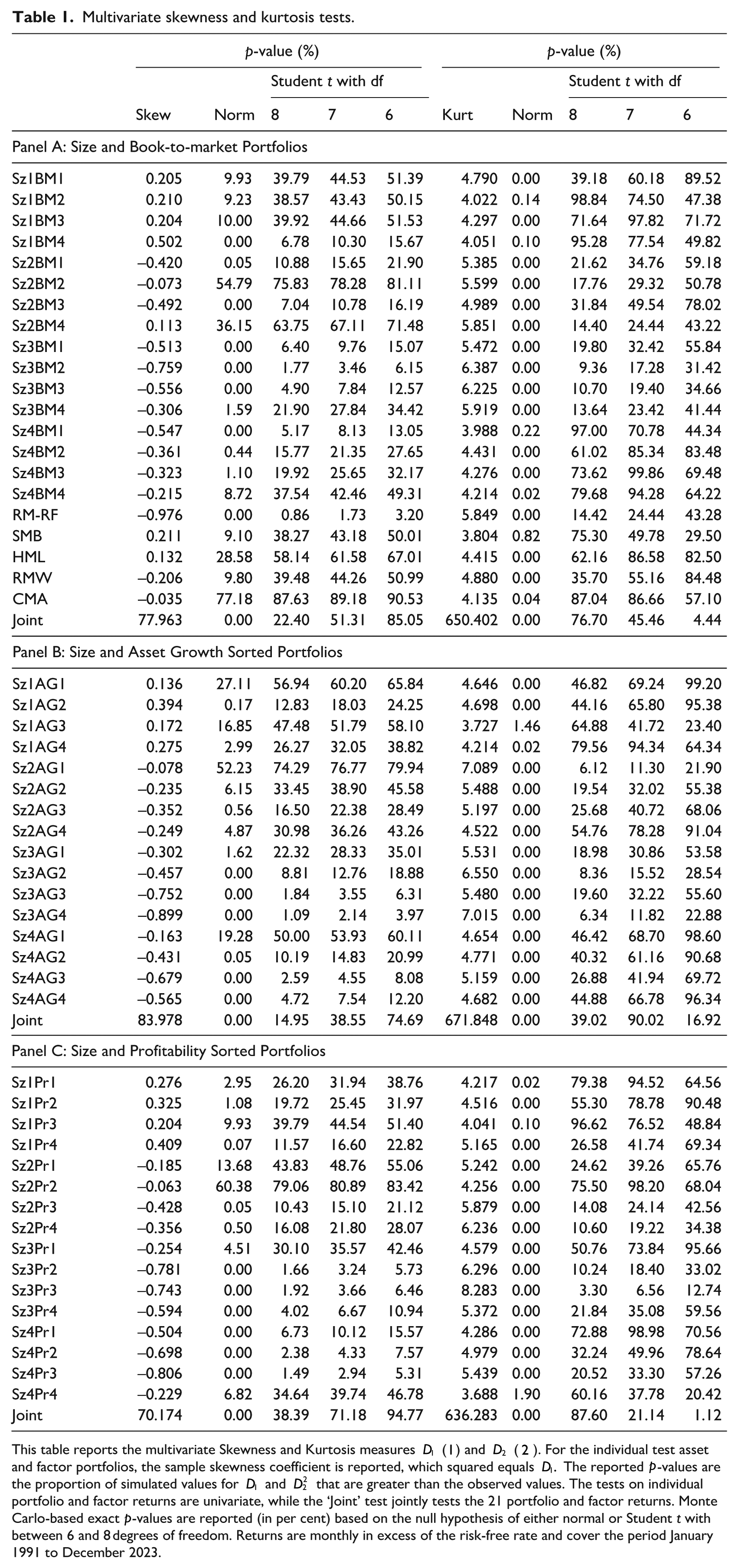
This table reports the multivariate Skewness and Kurtosis measures D₁ (1) and D₂ (2). For the individual test asset and factor portfolios, the sample skewness coefficient is reported, which squared equals D₁. The reported p-values are the proportion of simulated values for D₁ and $D_2^2$ that are greater than the observed values. The tests on individual portfolio and factor returns are univariate, while the ‘Joint’ test jointly tests the 21 portfolio and factor returns. Monte Carlo-based exact p-values are reported (in per cent) based on the null hypothesis of either normal or Student t with between 6 and 8 degrees of freedom. Returns are monthly in excess of the risk-free rate and cover the period January 1991 to December 2023.

Panel A of Table 1 shows very strong evidence of non-normality, and the evidence against normality is strongest in the kurtosis statistic D₂. The largest p-value for the kurtosis test D₂ is only 0.82%. For the size and book-to-market portfolio, the largest p-value is only 0.22% for the large-growth portfolio – 11 of the 16 portfolios are zero to four decimal places. If the data is normally distributed, the kurtosis statistic should equal three, but we see that every portfolio is greater than three by a large margin. Even the factors, with the exception of SMB, are well above four. The joint kurtosis test has a p-value that is smaller than one hundredth of 1%. The p-value of the test for kurtosis consistent with a multivariate Student t distribution with 6 degrees of freedom is also rejected (just) at the 5% level, but we are unable to reject the null that the size and book-to-market portfolios come from a multivariate t distribution with 7 or 8 degrees of freedom. Looking at the skewness tests, we find that small stocks are generally positively skewed, but larger stocks tend to be negatively skewed. Interestingly, the size and value factors are also positively skewed, but the profitability, asset growth, and market return factors are all negatively skewed too. Six of the 16 size and book-to-market portfolios have skewness that is not statistically different from zero at the 5% level, but of course we must be cautious about interpreting multiple comparisons and the multivariate tests. As Richardson and Smith (1993) note, when returns are highly correlated, as our portfolio returns are, misleading conclusions can be reached by focusing on univariate tests. The evidence against normality from observing two independent variables that have statistically significant univariate kurtosis is much less significant if the two variables are highly correlated, as a few extremely large returns that may occur by chance, leading to one asset’s return having large sample skewness, will also affect the other stock because of this correlation. Thus, inference should focus on joint tests. The joint test for kurtosis is reported in the final row and is 650. Since the statistic is computed using 21 test assets and 396 monthly observations, if returns and factors were really jointly normally distributed, the test statistic would be normally distributed with a mean of 483 and a standard deviation of 3.1. The multivariate kurtosis test statistic is thus 53.5 standard errors from zero for the size and book-to-market returns!

Interestingly, the four small stock portfolios tend to have smaller kurtosis than larger stock portfolios. An important reason for this is that the number of stocks used in the small portfolio is significantly larger. The four smallest stock portfolios average around 125 stocks each, while the four largest stock portfolios average around 25 stocks. If we construct portfolios by ranking stocks into four size bins with equal numbers of stocks and then into four book-to-market portfolios independently, the number of stocks in the Sz1BM1 portfolio is significantly lower, and the Kurtosis statistic jumps to 6.7. All four Sz1 portfolios’ skewness jumps markedly too, with the Sz1BM1 with independent homogeneous sorts having a skewness statistic of 0.881, which is much higher than 0.205 in the dependent heterogeneous size bins. Of course, the Sz1Bm1 homogeneous independent sort is $7 million. Indeed, if the small portfolio is defined as the 25% smallest stocks by market cap, the average firm size for all value portfolios is only around $7 million.

The joint skewness test convincingly rejects the null hypothesis that returns are normally distributed (p-value of 0.0001), but is unable to reject the null of a Student’s t distribution with between 6 and 8 degrees of freedom. Since the Student t, like the normal, are symmetric distribution, this suggests a lack of power in skewness to reject the student t distribution.

4. Asset pricing with fat tails

If the n-dimensional vector X_t is distributed as a multivariate t random variable, its probability density function is given by

$$\begin{array}{c}f\left(X_t|\mu ,\psi ,\nu \right)=\frac{\Gamma \left((\nu +n)/2\right)}{\Gamma \left(\nu /2\right){\left(\nu \pi \right)}^{n/2}{|\psi |}^{1/2}}{\left(1+\frac{1}{\nu }{\left(X_t-\mu \right)}^{\prime }{\psi }^{-1}\left(X_t-\mu \right)\right)}^{-(\nu +n)/2}.\end{array}$$

(7)

A feature of the multivariate t (MVT) density is that the tail probabilities decline at a polynomial rate rather than the exponential decay rate in the normal distribution, which means that the multivariate t distribution is fat-tailed. Because of this feature, the MVT distribution is used in the context of robust estimation and robust regression (Lange et al., 1989). It is well-known that MVT random variables can be expressed as a chi-square mixture of normal random variables

$$\begin{array}{c}{X}_t=\mu +{\Psi }^{1/2}{Z}_t/\sqrt{q_t},\end{array}$$

(8)

where Z_t in an n-dimensional standard normal random variable and $q_t\sim {\chi }_{\nu }^2/\nu$ is a scaled chi-square random variable that is independent of Z_t. The mixture of normal distributions provides an interesting way to understand excess kurtosis. The latent variable q_t captures the flow of information in this class of models. There are periods where new information is less than average, leading to returns closer to the mean, while in other time periods the amount of new information is atypically large, leading to outlying returns. This pattern of behaviour leads to more kurtosis than observed in a normal distribution with constant variance. Excess kurtosis induced by this heterogeneous information flow causes the sample mean, which is efficient when the latent scaling term is constant (and returns are thus normally distributed), to be inefficient because it places too much weight on extreme returns.

If returns and factors are distributed as multivariate t then parameter estimates that maximize the log-likelihood function based on that density will outperform estimates based on, for example, the normal density. In particular, when X_t is multivariate t log-likelihood function is given by

$$\begin{array}{c}\ln ℒ\left(\mu ,\Psi ,\nu ;X\right)=\mathrm{constant}-\frac{T}{2}\ln |\Psi |-\frac{\nu +n}{2}\sum _{t=1}^T\ln \left(1+\frac{{\left(X_t-\mu \right)}^{\prime }{\Psi }^{-1}\left(X_t-\mu \right)}{\nu }\right).\end{array}$$

(9)

A disadvantage of the non-normal distributions is that closed-form expressions for the maximum likelihood estimators are generally not available, requiring numerical optimization for estimating parameters. Indeed, the number of parameters involved, even for modest n can be quite daunting since there are n parameters for the mean vector and n(n + 1)/2 unique elements in Ψ. Further complicating numerical optimization is the need to impose the constraint that the scale matrix Ψ is positive definite.

However, for the multivariate t distribution the EM algorithm of Dempster et al. (1977) can be applied (Liu and Rubin, 1995) to provide a rapid iterative approach that converges monotonically to the optimal parameter estimates. The algorithm takes an initial guess for the mean vector and scale matrix, say ${\tilde{\mu }}^{(1)}=\widehat{\mu }$ and ${\tilde{\Psi }}^{(1)}=\tilde{\Psi }=\widehat{V}(\nu -2)/\nu$ , which allows iterative estimation via the following three equations:

$$\begin{array}{c}{u}_t^{\left(i\right)}=\frac{\nu +n}{\nu +{\left(X_t-{\tilde{\mu }}^{\left(i\right)}\right)}^{\prime }{\left({\tilde{\Psi }}^{\left(i\right)}\right)}^{-1}{\left(X_t-{\tilde{\mu }}^{\left(i\right)}\right)}^{\prime }}\end{array}$$

(10)

$$\begin{array}{c}{\tilde{\mu }}^{\left(i+1\right)}=\frac{{\sum }_{t=1}^T{u}_t^{\left(i\right)}{X}_t}{{\sum }_{t=1}^T{u}_t^{\left(i\right)}}\end{array}$$

(11)

$$\begin{array}{c}{\tilde{\Psi }}^{\left(i+1\right)}=\sum _{t=1}^T{u}_t^{\left(i\right)}\left(X_t-{\tilde{\mu }}^{\left(i+1\right)}\right){\left(X_t-{\tilde{\mu }}^{\left(i+1\right)}\right)}^{\prime }.\end{array}$$

(12)

The conditional mean is thus a weighted average of the sample returns, where the weights are

$$\begin{array}{c}{w}_t=\frac{u_t}{{\sum }_{t=1}^T{u}_t}\end{array}$$

(13)

where using the Mahalanobis distance between X_t and $\tilde{\mu }$ as

$${\delta }_t={\left(X_t-\tilde{\mu }\right)}^{\prime }{\left(\tilde{\Psi }\right)}^{-1}\left(X_t-\tilde{\mu }\right),$$

we can write

$$u_t=\frac{\nu +n}{\nu +{\delta }_t},$$

so the maximum likelihood estimator of the mean under a multivariate t distribution places less weight on more extreme observations, since u_t is a decreasing function of δ_t.

As an aside, the estimation algorithm works by casting the multivariate t as an inverted Gamma mixture of normal distributions, and then u_t is the expected value of this mixing scale conditional on X_t and the mean and scale matrix. Heuristically, we can motivate it by taking the derivative of (6) with respect to μ setting equal to zero, multiplying both sides by Ψ and simplifying gives

$$\begin{array}{c}\mu =\frac{{\sum }_{t=1}^T\frac{\nu +n}{\nu +{\delta }_t}{X}_t}{{\sum }_{t=1}^T\frac{\nu +n}{\nu +{\delta }_t}}.\end{array}$$

(14)

So when the Mahalanobis distance of X_t from the mean is large, those observations are given a smaller weight. When the data is normal, the weight on each observation is constant and thus independent of the size of the X_t s. However, when returns are from a multivariate t distribution with finite degrees of freedom, then outliers occur more frequently than they would if the data were normal, and the sample average performs less efficiently than the maximum likelihood estimator because it is adversely affected by such outliers. The sample average in this case will be consistent and asymptotically normal, but it will be less efficient than maximum likelihood estimates because these optimally place less weight on extreme values, resulting in improved efficiency. Indeed, Lange et al. (1989) discuss using the multivariate t distribution as an explicit way to construct robust estimates of multivariate means and covariance matrices and multiple regressions in the presence of outliers.

Proposition 4 of Lange et al. (1989) shows that the asymptotic covariance matrix of $\tilde{\mu }$ when v > 2 is

$$\begin{array}{c}Avar\left(\tilde{\mu }\right)=\frac{\nu +n+2}{\nu +n}\Psi .\end{array}$$

(15)

The asymptotic covariance matrix of the sample mean when the data are iid, equals its covariance matrix V. When the data is multivariate t then if v > 2 then V = v/(v − 2)Ψ, giving

$$\begin{array}{c}Avar\left(\widehat{\mu }\right)=\frac{\nu }{\nu -2}\Psi .\end{array}$$

(16)

In each case, we consider there are 16 test assets and 5 factors, so n = 21 and if v = 7, which seems to fit the data reasonably well, then the asymptotic standard errors for the sample average will be 14.3% larger than the standard errors for the maximum likelihood estimates, which is quite significant.

An advantage of allowing for non-normality by using the multivariate t distribution is that the standard Capital Asset Pricing Model (CAPM) of Sharpe (1964) and Lintner (1965) because it is a member of the broader class of elliptical distributions and the standard CAPM will hold for this class of multivariate distributions (Chamberlain, 1983; Owen and Rabinovitch, 1983). This enables us to test the performance of asset pricing models using a conditional distribution that is both tractable and justifiable theoretically, and yet can also account for the significant departures from multivariate normality we see in equity returns. And the Australian stock market is no different from other markets, and indeed, the large number of very small stocks suggests that non-normality is particularly relevant to the Australian empirical experience.

The components of X_t consist of r_t, the N-vector of asset returns; and f_t, the K-vector of factor returns, and we let ε_t be an N-vector of zero mean regression errors with nonsingular covariance matrix ∑ giving the factor structure

$$\begin{array}{c}{r}_t=\alpha +\beta f_t+{\epsilon }_t.\end{array}$$

(17)

The parameters of the regression model are related to the moment for $X_t={({r^{\prime }}_t,{f^{\prime }}_t)}^{\prime }$ using the partition:

$$\begin{array}{c}\mu =\left[\begin{array}{c}{\mu }_1\\ {\mu }_2\end{array}\right]V=\left[\begin{array}{cc}{V}_{11}& V_{12}\\ V_{21}& V_{22}\end{array}\right]\end{array}$$

(18)

When both f_t and ε_t are normally distributed then r_t and f_t are jointly normal, and the conditional distribution of r_t given f_t is well-known, having a conditional mean

$$\begin{array}{c}E(r_t|f_t)={\mu }_1+V_{12}{V}_{22}^{-1}(f_t-{\mu }_2)\end{array}$$

(19)

and covariance matrix

$$\begin{array}{c}V\left(r_t|f_t\right)=V_{11}-V_{12}{V}_{22}^{-1}{V}_{21}=\Sigma .\end{array}$$

(20)

And we also have

$$\begin{array}{c}\alpha ={\mu }_1-V_{12}{V}_{22}^{-1}{\mu }_2,\beta =V_{12}{V}_{22}^{-1}.\end{array}$$

(21)

As Kan and Zhou (2017) note, when returns and factors are multivariate normal, then ∑ is the covariance matrix of ε_t conditional on f_t, but when both r_t and f_t is a jointly multivariate t random variable

$$\begin{array}{c}Var\left(r_t|f_t\right)=\left(\frac{\nu -2+{\left(f_t-{\mu }_2\right)}^{\prime }{V}_{22}^{-1}(f_t-{\mu }_2)}{\nu +K-2}\right)\Sigma \end{array}$$

(22)

showing that the conditional variance of r_t given f_t is not constant but is rather heteroscedastic. This is in contrast to the standard approach of modelling a regression in which the errors follow a student t distribution conditional on the regressors. As such, the regressors and the errors are independent. This class of models has been used in robust estimation because it downweights extreme observations (see, for example, Lange et al. (1989)). In cases where the exogenous variables are chosen by the researcher, this specification makes sense. In the context of asset pricing factor models, jointly modelling factors and returns as jointly multivariate t random variables arguably makes more sense. As noted above one can view the multivariate t as an inverse chi-square mixture of normals, so the leptokurtosis arises because on some days there is much less information than normal resulting in observations clustered around the mean, while on other days the amount of information, and hence variance, is much greater and this results in too many returns far from the mean (Blattberg and Gonedes, 1974). (Too many is measured relative to the normal distribution with the same mean and covariance matrix.) The joint multivariate t specification can be motivated as the volume of information flow affects all portfolio and factor returns, as they are all simply portfolios of component stock returns. Using this information flow interpretation to have regressors that are multivariate t random variables independent of the regression errors that are also multivariate t requires that the amount of systematic information (that affects factor returns) on any given day be independent of the amount of common idiosyncratic information (affecting the errors). This, while possible, is harder to motivate conceptually.

The key distinction between these two specifications is the conditional heteroscedasticity, and this heteroscedasticity has a specific functional form. In Appendix A, we present a GMM-test of the overidentifying moment condition $E(({\epsilon }_{it}^2-{\sigma }_i^2){\delta }_t)=0$ for i = 1,…,N, which is distributed as chi-square with N degrees of freedom under the null.

Alternatively, we can test between the two using a likelihood ratio type test. Unfortunately, the two models are non-nested, meaning that one model cannot be expressed as a restriction on the parameters of the more general model. When models are nested, then twice the difference in the log-likelihoods follows a chi-square distribution with degrees of freedom equal to the number of restrictions. However, Vuong (1999) shows that when two models, 1 and 2, are non-nested (as in the case of multivariate t errors versus multivariate t returns), then the test statistic

$$\begin{array}{c}V=\frac{L_1-L_2-\frac{\left(K_1-K_2\right)}{2}\ln T}{T\omega }\end{array}$$

(23)

where L_i is the log-likelihood of the model i, K_i is the number of parameters in the model i and ω is an estimate of the variance of the difference in the log densities of models 1 and 2, and can be used to conduct inference. In particular, under the null hypothesis that both models are equivalent (the expected value of the log-likelihoods is equal), the test statistic V will be asymptotically distributed as a standard normal random variable. When model 1 fits the data better, V will diverge V → ∞, while model 2 fits the data better then V → −∞.

When returns are multivariate t and we have the estimates $\tilde{\mu }$ and $\tilde{\Psi }$ then the maximum likelihood estimates of the betas and alphas are given by

$$\begin{array}{c}\tilde{\beta }={\tilde{\Psi }}_{12}{\tilde{\Psi }}_{22}^{-1}\end{array}$$

(24)

and

$$\begin{array}{c}\tilde{\alpha }={\tilde{\mu }}_1-\tilde{\beta }{\tilde{\mu }}_2.\end{array}$$

(25)

.

Kan and Zhou (2017) show that the asymptotic covariance matrix of the least squares and maximum likelihood estimates of the alphas and betas when the returns and factors are jointly multivariate t random variables with v degrees of freedom are:

$$\begin{array}{c}Avar\left[\begin{array}{c}\tilde{\alpha }\\ vec(\tilde{\beta })\end{array}\right]=\left(\frac{\nu +n+2}{\nu +n}\right)\left[\begin{array}{cc}\left(\frac{\nu -2}{\nu }\right)+{{\mu }^{\prime }}_2{V}_{22}^{-1}{\mu }_2& -{{\mu }^{\prime }}_2{V}_{22}^{-1}\\ -V_{22}^{-1}{\mu }_2& V_{22}^{-1}\end{array}\right]\otimes \Sigma \end{array}$$

(26)

and

$$\begin{array}{c}Avar\left[\begin{array}{c}\widehat{\alpha }\\ vec(\widehat{\beta })\end{array}\right]=\left[\begin{array}{cc}1+\left(\frac{\nu -2}{\nu -4}\right){{\mu }^{\prime }}_2{V}_{22}^{-1}{\mu }_2& -\left(\frac{\nu -2}{\nu -4}\right){{\mu }^{\prime }}_2{V}_{22}^{-1}\\ -\left(\frac{\nu -2}{\nu -4}\right)V_{22}^{-1}{\mu }_2& \left(\frac{\nu -2}{\nu -4}\right)V_{22}^{-1}\end{array}\right]\otimes \Sigma \end{array}$$

7)

respectively.

The ratio of the asymptotic variance of the two β estimates are given by

$$\begin{array}{c}\frac{Avar(vec(\tilde{\beta }))}{Avar(vec(\widehat{\beta }))}=\left(\frac{\nu +n+2}{\nu +n}\right)\left(\frac{\nu -2}{\nu -4}\right),\end{array}$$

(28)

and thus the standard errors of $\tilde{\beta }$ are 19.2% lower than the standard errors of the OLS estimate $\widehat{\beta }$ when returns and factors are multivariate t. Just as in the normally distributed case, the variance of $\widehat{\alpha }$ and $\tilde{\alpha }$ depend on the squared Sharpe ratio of the factors, and we express the ratio of the asymptotic variance of the two estimators of α as

$$\begin{array}{c}\frac{Avar(\tilde{\alpha })}{Avar(\widehat{\alpha })}=\frac{\left(\frac{\nu +n+2}{\nu +n}\right)\left(\frac{\nu -2}{\nu }\right)+\left(\frac{\nu +n+2}{\nu +n}\right){{\mu }^{\prime }}_2{V}_{22}^{-1}{\mu }_2}{1+\left(\frac{\nu -2}{\nu -4}\right){{\mu }^{\prime }}_2{V}_{22}^{-1}{\mu }_2},\end{array}$$

(29)

clearly showing this dependence on the squared Sharpe ratio. We can gauge the possible improvement in efficiency by noting that the ratio is bounded between $(\frac{\nu +n+2}{\nu +n})(\frac{\nu -2}{\nu })$ as ${{\mu }^{\prime }}_2{V}_{22}^{-1}{\mu }_2\to 0$ and $(\frac{\nu +n+2}{\nu +n})(\frac{\nu -4}{\nu -2})$ as ${{\mu }^{\prime }}_2{V}_{22}^{-1}{\mu }_2\to \infty .$ In our case with n = 21 and if v = 7 the reduction in the standard errors of $\tilde{\alpha }$ compared with $\widehat{\alpha }$ is between 12.5% and 19.8% as ${{\mu }^{\prime }}_2{V}_{22}^{-1}{\mu }_2$ varies between zero and infinity. There are thus significant efficiency gains available by estimating the parameters of factor pricing models when the returns and factors are multivariate t random variables.

This raises the question of how to test the efficiency of the factors f_t when returns are non-normal. The standard approach to testing asset pricing models follows Gibbons et al. (1989), who test the parametric restriction

$$H_0:\alpha =0.$$

When the factor model residuals ε_t are normally distributed, this hypothesis is tested using the GRS statistics

$$\begin{array}{c}GRS=\frac{T-N-k}{N}\frac{{\widehat{\alpha }}^{\prime }{\widehat{\Sigma }}^{-1}\widehat{\alpha }}{1+{{\widehat{\mu }}^{\prime }}_2{\widehat{V}}_{22}^{-1}{\widehat{\mu }}_2}~F_{N,T-N-K}.\end{array}$$

(30)

However, when returns and factors are multivariate t random variables, the GRS test is not appropriate. Zhou (1993) shows that the distribution of the GRS test statistic and the distribution of the OLS estimates vary only slightly when residuals are assumed to be either normally or multivariate t random variables. However, when the distribution of the market returns is taken into account, allowing returns to be multivariate t the distribution of the test statistics and the estimates of the GRS statistic and the regression parameter estimates are markedly different. He also shows that accounting for non-normality leads to higher p-values for the GRS test statistic, indicating that failing to account for non-normality biases the GRS test into rejecting asset pricing models. Indeed, Zhou (1993) shows that assuming normality when constructing critical values rejects the CAPM, but allowing for non-normality results in the GRS test no longer rejecting the CAPM in some situations.

MacKinlay and Richardson (1991) construct a GMM-based Wald test of the zero alpha restriction that doesn’t place distributional assumptions like normality. It is the asymptotic version of the GRS statistic, leading to a chi-square rather than F distribution under the null hypothesis. They also allow returns to be multivariate t random variables, noting the residual heteroscedasticity that this entails, and quantifying the bias in the GRS statistic that arises by erroneously assuming normality. The test continues to use the OLS estimates of the alphas, which we have seen from Zhou (1993) and Kan and Zhou (2017), are inefficient when the data is not multivariate t.

Kan and Zhou (2017) developed a likelihood ratio test to replace the GRS test when returns and factors are multivariate t random variables. They develop an EM algorithm to estimate the other model parameters while imposing the restrictions of the null hypothesis that α = 0 the null hypothesis using the following mapping

$$\begin{array}{c}\mu =\left[\begin{array}{c}\beta {\mu }_2\\ {\mu }_2\end{array}\right]\end{array}$$

(31)

$$\begin{array}{c}\Psi =\left[\begin{array}{cc}\beta {\Psi }_{22}{\beta }^{\prime }+{\Psi }_{\epsilon }& \beta {\Psi }_{22}\\ {\Psi }_{22}{\beta }^{\prime }& {\Psi }_{22}\end{array}\right]\end{array}$$

(32)

where Ψ _ε = (v − 2)/v∑. Appendix C describes the EM algorithm used to estimate the maximum likelihood parameter estimates under the null of zero alphas. Denoting the restricted maximum likelihood estimates of the parameters by ${\tilde{\mu }}_r$ and ${\tilde{\Psi }}_r$ , then the likelihood ratio test is given by

$$\begin{array}{c}LRT\equiv 2\left(\frac{T-N/2-K-1}{T}\right)\left[\log ℒ(\tilde{\mu },\tilde{\Psi })-\log ℒ({\tilde{\mu }}_r,\widetilde{{\Psi }_{\mathrm{r}}})\right]\begin{array}{c}A\\ ~\end{array}{\chi }_N^2\end{array}$$

(33)

where $\log \mathcal{L}(\tilde{\mu },\tilde{\Psi })$ is the log-likelihood function under the multivariate t distribution, and we use the Bartlett correction factor (T − N)/(2 − K − 1) rather than T.

5. Results

We use the portfolio and factor returns to estimate and test multiple factor models using Australian returns that assume normality or a multivariate t distribution for factors and returns. Table 2 reports the maximum likelihood estimates of the means and standard deviations of the test assets and factors under these two distributional assumptions. The sample mean is the maximum likelihood estimate of the mean under the assumption of normality. The results are largely as expected. Within each size bin, we see sample excess returns increasing as portfolios move from growth to value (BM1 to BM4); decreasing, but not monotonically, from conservative to aggressive asset growth (AG1 to AG4); and increasing from weak to robust profitability (Pr1 to Pr4). We also find that standard deviations decrease within each size bucket as we increase all three non-size characteristics.

Table 2.

Maximum likelihood estimates of means and standard deviations under alternative distributional assumptions.

	Mean				Standard deviation
	Norm	Student t with df			Norm	Student t with df
		8	7	6		8	7	6
Panel A: 16 Portfolios Sorted on Size and Book-to-Market Ratio
Sz1BM1	0.681	−0.110	−0.135	−0.162	8.933	8.659	8.829	9.090
Sz1BM2	1.067	0.395	0.373	0.350	8.302	8.137	8.295	8.539
Sz1BM3	1.096	0.395	0.376	0.355	8.091	7.830	7.984	8.221
Sz1BM4	1.308	0.610	0.589	0.567	7.956	7.806	7.958	8.192
Sz2BM1	0.357	−0.132	−0.149	−0.166	7.133	7.113	7.258	7.478
Sz2BM2	0.462	−0.016	−0.031	−0.047	6.566	6.460	6.589	6.786
Sz2BM3	0.393	0.114	0.104	0.093	5.551	5.702	5.821	6.002
Sz2BM4	0.777	0.456	0.446	0.437	5.998	5.926	6.045	6.227
Sz3BM1	0.458	0.157	0.144	0.130	6.851	6.919	7.061	7.278
Sz3BM2	0.511	0.362	0.356	0.350	5.292	5.382	5.493	5.662
Sz3BM3	0.351	0.149	0.141	0.132	5.323	5.392	5.504	5.674
Sz3BM4	0.717	0.476	0.467	0.458	5.564	5.523	5.634	5.804
Sz4BM1	0.462	0.366	0.362	0.358	4.336	4.649	4.753	4.908
Sz4BM2	0.302	0.134	0.129	0.124	4.408	4.609	4.710	4.862
Sz4BM3	0.451	0.286	0.280	0.272	4.397	4.643	4.743	4.894
Sz4BM4	0.805	0.667	0.665	0.663	4.942	5.053	5.159	5.320
RM-RF	0.513	0.380	0.375	0.370	3.674	3.817	3.901	4.027
SMB	0.192	−0.103	−0.112	−0.120	3.953	3.963	4.044	4.168
HML	0.437	0.454	0.457	0.461	3.326	3.269	3.333	3.432
RMW	0.278	0.479	0.486	0.493	3.680	3.508	3.576	3.680
CMA	0.504	0.521	0.520	0.518	2.826	2.836	2.893	2.981
Panel B: 16 Portfolios Sorted on Size and Asset Growth
Sz1AG1	0.988	0.424	0.404	0.383	9.188	8.963	9.140	9.411
Sz1AG2	1.302	0.731	0.712	0.691	7.985	7.762	7.913	8.147
Sz1AG3	1.142	0.609	0.590	0.568	7.656	7.657	7.811	8.047
Sz1AG4	0.689	0.136	0.116	0.094	8.567	8.414	8.580	8.836
Sz2AG1	0.940	0.572	0.559	0.544	6.865	6.603	6.736	6.939
Sz2AG2	0.639	0.420	0.411	0.400	5.293	5.365	5.474	5.641
Sz2AG3	0.554	0.361	0.352	0.343	5.979	6.052	6.176	6.363
Sz2AG4	−0.145	−0.521	−0.535	−0.549	7.321	7.288	7.434	7.658
Sz3AG1	0.617	0.342	0.331	0.320	5.578	5.678	5.797	5.976
Sz3AG2	0.795	0.749	0.746	0.743	5.055	5.002	5.104	5.258
Sz3AG3	0.350	0.260	0.254	0.248	5.327	5.515	5.632	5.809
Sz3AG4	0.211	0.107	0.101	0.095	6.995	6.935	7.074	7.286
Sz4AG1	0.798	0.673	0.669	0.664	4.300	4.474	4.569	4.711
Sz4AG2	0.671	0.610	0.607	0.603	4.051	4.199	4.289	4.424
Sz4AG3	0.245	0.220	0.219	0.217	4.475	4.613	4.710	4.856
Sz4AG4	0.423	0.267	0.262	0.256	5.232	5.311	5.423	5.592
RM-RF	0.513	0.439	0.435	0.432	3.674	3.772	3.854	3.975
SMB	0.192	−0.039	−0.046	−0.053	3.953	3.970	4.052	4.177
HML	0.437	0.478	0.482	0.487	3.326	3.318	3.384	3.485
RMW	0.278	0.457	0.464	0.472	3.680	3.498	3.565	3.669
CMA	0.504	0.492	0.491	0.490	2.826	2.832	2.889	2.976
Panel C: 16 Portfolios Sorted on Size and Profitability
Sz1Pr1	0.553	−0.222	−0.243	−0.265	9.695	9.474	9.659	9.943
Sz1Pr2	0.907	0.255	0.237	0.218	9.100	8.989	9.166	9.438
Sz1Pr3	1.230	0.430	0.410	0.389	9.084	8.839	9.009	9.271
Sz1Pr4	1.286	0.865	0.852	0.838	6.031	5.924	6.040	6.219
Sz2Pr1	0.092	−0.333	−0.344	−0.357	8.029	7.890	8.046	8.285
Sz2Pr2	0.406	−0.038	−0.047	−0.057	7.430	7.456	7.606	7.836
Sz2Pr3	0.288	0.079	0.074	0.068	5.471	5.477	5.588	5.757
Sz2Pr4	1.044	0.861	0.856	0.850	4.994	4.949	5.048	5.200
Sz3Pr1	−0.009	−0.187	−0.191	−0.195	7.507	7.657	7.815	8.055
Sz3Pr2	0.467	0.367	0.366	0.366	5.760	5.770	5.884	6.060
Sz3Pr3	0.554	0.437	0.433	0.430	4.816	4.783	4.880	5.028
Sz3Pr4	0.829	0.688	0.685	0.683	5.218	5.305	5.415	5.582
Sz4Pr1	0.648	0.467	0.463	0.459	5.483	5.615	5.733	5.911
Sz4Pr2	0.207	0.149	0.147	0.145	4.335	4.401	4.492	4.630
Sz4Pr3	0.435	0.380	0.378	0.376	4.332	4.501	4.598	4.743
Sz4Pr4	0.600	0.511	0.509	0.506	4.133	4.388	4.483	4.624
RM-RF	0.513	0.443	0.442	0.440	3.674	3.765	3.845	3.966
SMB	0.192	−0.084	−0.090	−0.097	3.953	3.958	4.039	4.162
HML	0.437	0.442	0.442	0.443	3.326	3.302	3.366	3.464
RMW	0.278	0.478	0.483	0.488	3.680	3.507	3.575	3.680
CMA	0.504	0.520	0.518	0.515	2.826	2.830	2.887	2.974

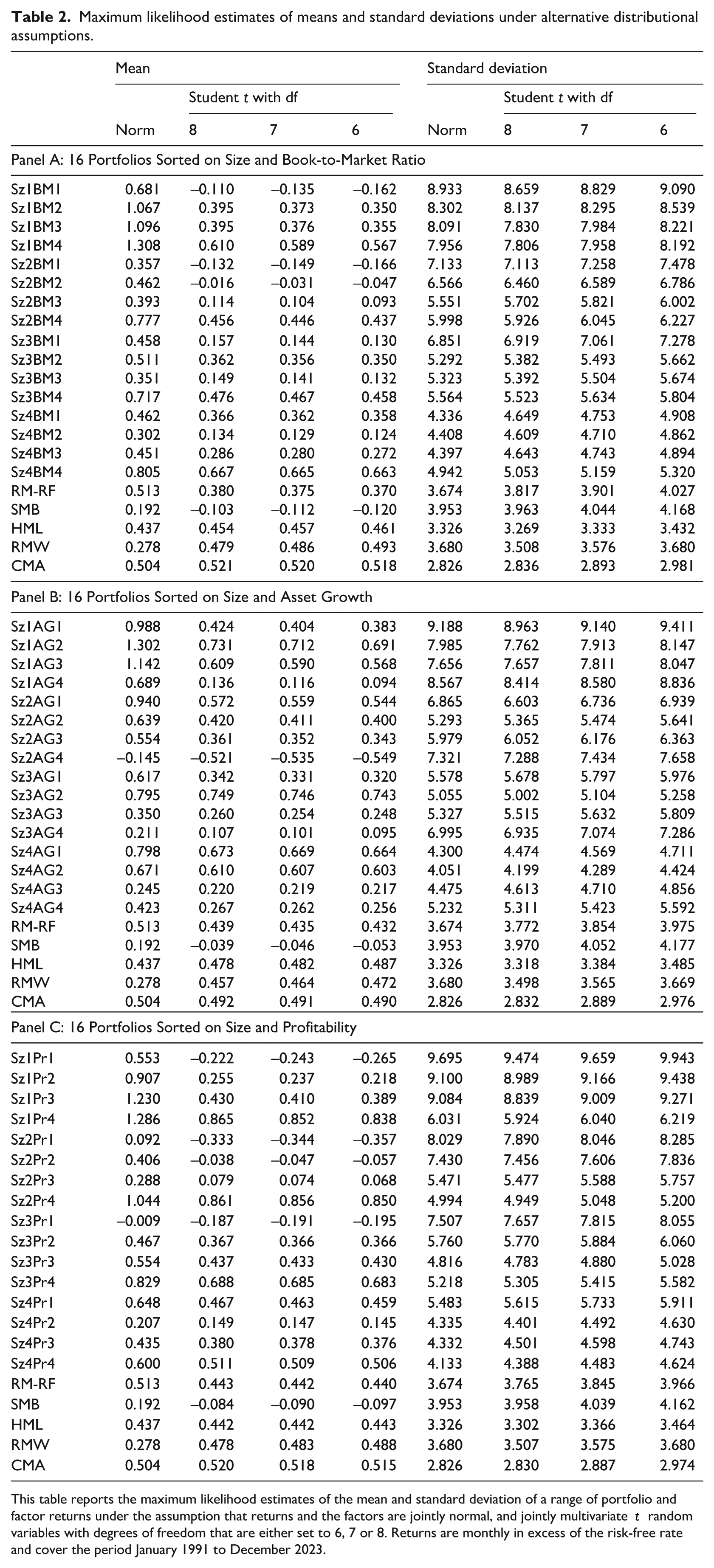
This table reports the maximum likelihood estimates of the mean and standard deviation of a range of portfolio and factor returns under the assumption that returns and the factors are jointly normal, and jointly multivariate t random variables with degrees of freedom that are either set to 6, 7 or 8. Returns are monthly in excess of the risk-free rate and cover the period January 1991 to December 2023.

These results are only statistically efficient if returns are normally distributed, because the sample average is not the maximum likelihood estimator of the mean when returns are non-normal. We can relax this assumption by estimating the means and standard deviations when returns and factors are jointly distributed as a multivariate t random variable. We also report those results in Table 2. We consider three different degrees of freedom: 6, 7 and 8. We find that 7 degrees of freedom seem to fit the data best based on the multivariate skewness and kurtosis tests discussed earlier, and considering values slightly higher and slightly lower allows us to gauge how robust the results are to varying the degrees of freedom. Relaxing the normality assumption on expected returns has a remarkable impact on the size and book-to-market sorted portfolios. The mean return on the small growth stock portfolio (Sz1Bm1) decreases from 68 basis points per month to -14 basis points per month – a change of over 0.8% per month or about 10% per year! The decrease in expected returns among the four largest portfolios only drops 0.1% to 0.2% per month. The value effect is still strongly observable. For example, among the smallest stocks, the spread between the extreme value and growth portfolios is over 0.6% per month if returns are assumed to be normal and over 0.7% if returns are student t with 7 degrees of freedom. The spread for the largest four portfolios drops from 0.34% to 0.30%, with all returns being at a slightly lower level.

All portfolio mean returns are lower when student t distributions are used rather than normal returns because the most extreme positive returns are when the Mahalanobis distance δ_t is largest. And it is especially true that returns on small-cap stocks tend to be much higher during months that are more extreme. If we calculate the average return on the 5% days with the largest δ_t, which are when δ_t > 65, the average monthly percentage return on the small growth stock is 7.64% per month. On months where δ_t ≤ 64 the mean excess return was 0.29% per month. That is a difference of 25 times! This pattern is similar for the other small stock portfolios, all having average returns of between 5% and 7% per month during the months where the Mahalanobis distance is greatest. The quadratic loss function that comes with the normality assumption places too much weight on these extreme observations, because such extreme outcomes simply don’t arise frequently when returns are normal, but happen relatively frequently when returns exhibit fat tails, as in the multivariate t distribution. These effects are seen also in the scatter plot of the Mahalanobis distance against the returns for the Small-Growth portfolio, the market and SMB factor returns in Figure 1. We see a large number of observations with high returns when δ_t is between 80 to 100. And for the SMB, the ratio of positive to negative returns when δ_t is above about 75 looks to be roughly two-to-one. When all these larger returns are down-weighted, the estimates of the means are moderated. Again, this is statistically optimal because the sample average places far too much weight on extreme outcomes because if the data truly is normal, such large outcomes simply don’t occur, however, outliers are common when dealing with leptokurtic distributions such as the multivariate t distribution.

Figure 1.

Scatter plot of small-growth stocks, market and size factor returns against δ_t.

This dramatic change in signs is even larger than that observed in the United States returns. For example, Kan and Zhou (2017) note that the smallest size and book-to-market portfolio’s conditional mean decreases by 2% annually when estimated by maximum likelihood using a Student t rather than a normal. In Australia, the difference in estimates is closer to 9% annually. This is because the smallest stocks in the Australian market are microscopic relative to US firms. However, the difference in the size and book-to-market portfolio for growth stocks that are between the 75th and 90th percentiles by market capitalization (Sz3Bm1), the difference between the normal and t maximum likelihood estimates of the mean are over 3.5% annually.

Similar results hold for the other sorting strategies. To illustrate, for the profitability-sorted stocks, the drop in estimated mean returns when using a multivariate t distribution with finite degrees of freedom is marked. The average decrease in mean returns for the four small-size portfolios is about 70 basis points per month. The profitability effect is still amplified: under normal returns, the spread Sz1Pr4-Sz1Pr1 is about 75 basis points, but for a student t distribution with 7 degrees of freedom, the same spread is 110 basis points per month.

Interestingly, the estimates of the factor prices of risk, other than the size factor SMB, don’t change dramatically when excess kurtosis is accounted for. The excess returns to the market, HML and CMA are all about, or for HML slightly below, 50 basis points per month when returns are normal, and they are all between 44 and 48 basis points if we assume a Student t distribution with 7 degrees of freedom and estimate them jointly with the Profitability sorted portfolios. And RMW’s price of risk increases from 28 to 48 basis points. However, the size factor drops from 19 basis points to negative 10 basis points. A 30 basis point swing flipping the sign is the most striking result that we find. Note also that the maximum likelihood estimates of the factor means under the multivariate t assumption vary as the assets change because although the estimates are a weighted average of that factor’s returns, varying the asset portfolio returns will cause variations in the weights and result in small variations across specifications.

Interestingly, the standard deviations don’t change appreciably when fat tails are accounted for. Table 3 reports the fitted maximum likelihood estimates of the betas for the three-factor model for all three portfolio formation strategies. Interestingly, we find that the distributional assumptions have very little impact on the betas, which stands in stark contrast to the profound impact on the estimates of alpha. This is consistent with the results in Table 2 that find very little impact on the estimates of the standard deviations.

Table 3.

Portfolio betas from the three-factor model for 16 size and book-to-market portfolios.

	RM-RF		SMB		HML
	Norm	T(7)	Norm	T(7)	Norm	T(7)
Panel A: Size and Book-to-Market Sorted Portfolios
Sz1BM1	1.153	1.236	1.433	1.376	−0.242	−0.174
Sz1BM2	1.170	1.229	1.352	1.345	0.017	0.118
Sz1BM3	1.066	1.120	1.343	1.299	0.251	0.268
Sz1BM4	1.016	1.059	1.282	1.282	0.338	0.407
Sz2BM1	1.088	1.109	0.972	0.998	−0.410	−0.381
Sz2BM2	1.094	1.094	0.922	0.970	0.022	0.063
Sz2BM3	0.962	1.006	0.698	0.775	0.139	0.179
Sz2BM4	0.972	0.997	0.768	0.821	0.486	0.502
Sz3BM1	1.273	1.291	0.608	0.613	−0.379	−0.358
Sz3BM2	1.042	1.030	0.372	0.426	−0.163	−0.158
Sz3BM3	1.107	1.128	0.399	0.435	0.152	0.164
Sz3BM4	1.117	1.124	0.456	0.500	0.417	0.434
Sz4BM1	0.949	0.946	−0.168	−0.202	−0.451	−0.488
Sz4BM2	1.020	1.019	−0.121	−0.126	−0.098	−0.093
Sz4BM3	1.000	1.029	−0.067	−0.045	0.091	0.141
Sz4BM4	1.059	1.087	−0.025	−0.054	0.627	0.679
Panel B: Size and Asset Growth Sorted Portfolios
Sz1AG1	1.140	1.200	1.556	1.506	0.043	0.132
Sz1AG2	1.024	1.072	1.362	1.337	0.121	0.193
Sz1AG3	1.136	1.180	1.201	1.206	0.116	0.171
Sz1AG4	1.148	1.191	1.354	1.358	−0.016	0.076
Sz2AG1	0.991	1.012	0.968	0.950	0.144	0.179
Sz2AG2	0.902	0.919	0.693	0.743	0.188	0.200
Sz2AG3	1.045	1.028	0.767	0.858	−0.031	−0.034
Sz2AG4	1.208	1.216	0.982	1.025	−0.105	−0.060
Sz3AG1	1.117	1.121	0.474	0.521	0.135	0.132
Sz3AG2	1.039	1.042	0.393	0.399	0.061	0.069
Sz3AG3	1.070	1.097	0.382	0.419	−0.065	−0.052
Sz3AG4	1.326	1.288	0.595	0.620	−0.144	−0.109
Sz4AG1	0.953	0.972	−0.133	−0.132	0.120	0.152
Sz4AG2	0.936	0.937	−0.115	−0.108	−0.050	−0.042
Sz4AG3	1.024	1.023	−0.126	−0.121	−0.012	0.042
Sz4AG4	1.163	1.147	0.024	−0.040	−0.067	−0.078
Panel C: Size and Profitability Sorted Portfolios
Sz1Pr1	1.263	1.312	1.628	1.607	−0.030	0.028
Sz1Pr2	1.110	1.175	1.535	1.537	0.029	0.119
Sz1Pr3	1.266	1.338	1.399	1.374	0.099	0.207
Sz1Pr4	0.871	0.885	0.941	0.951	0.154	0.231
Sz2Pr1	1.175	1.161	1.099	1.149	−0.202	−0.157
Sz2Pr2	1.175	1.230	1.005	1.023	0.088	0.120
Sz2Pr3	0.939	0.949	0.684	0.740	0.198	0.247
Sz2Pr4	0.900	0.892	0.654	0.698	0.077	0.079
Sz3Pr1	1.304	1.352	0.739	0.784	−0.174	−0.103
Sz3Pr2	1.171	1.156	0.432	0.457	0.077	0.100
Sz3Pr3	1.019	1.012	0.359	0.364	0.073	0.052
Sz3Pr4	1.074	1.089	0.395	0.418	−0.025	−0.039
Sz4Pr1	1.196	1.221	0.021	−0.030	0.174	0.222
Sz4Pr2	1.022	1.004	−0.026	−0.039	0.066	0.079
Sz4Pr3	1.020	1.024	−0.090	−0.086	0.053	0.075
Sz4Pr4	0.937	0.946	−0.214	−0.205	−0.155	−0.160

This table reports the maximum likelihood estimates of the slope coefficients or betas from the Fama and French (1993) three-factor model for portfolios sorted based on size and Book-to-Market ratios under the assumption that returns are normally distributed and that returns and the factors are jointly multivariate t random variables with 7 degrees of freedom. Returns are monthly in excess of the risk-free rate and cover the period January 1991 to December 2023.

Table 4 reports the alphas for four models: the one-factor Capital Asset Pricing Model, the three-factor model of Fama and French (1993), the five-factor model of Fama and French (2015) that adds profitability and asset growth to the three-factor model, and a four-factor model (labelled as FF4) that is inspired by the Hou et al. (2015) ² that includes a market, size, profitability and investment factor. As the table shows the magnitudes of the alphas vary remarkably depending on whether one uses simple sample moments, which are only MLEs if returns are normal, or if we assume returns and factors exhibit kurtosis following the multivariate t distribution with 7 degrees of freedom. For the size and book-to-market sorted portfolios, the Sz1Bm1 portfolio goes from trivially negative (−0.036) to a much larger negative alpha (−0.645) in the CAPM and FF3 models, and in the FF5, the alphas switch signs from 0.107 to −0.131. The evidence against the CAPM is stronger if one imposes normality.

Table 4.

Portfolio alphas.

	CAPM		FF3		FF4		FF5
	Norm	T(7)	Norm	T(7)	Norm	T(7)	Norm	T(7)
Panel A: Size and Book-to-Market Sorted Portfolios
Sz1BM1	−0.036	−0.649	−0.080	−0.381	0.009	−0.227	0.107	−0.131
Sz1BM2	0.355	−0.142	0.199	0.003	0.391	0.294	0.392	0.280
Sz1BM3	0.444	−0.066	0.180	−0.025	0.469	0.352	0.382	0.270
Sz1BM4	0.690	0.163	0.393	0.139	0.593	0.490	0.489	0.351
Sz2BM1	−0.293	−0.589	−0.209	−0.291	−0.127	−0.122	0.012	0.012
Sz2BM2	−0.176	−0.476	−0.287	−0.358	−0.032	−0.079	−0.050	−0.099
Sz2BM3	−0.155	−0.301	−0.296	−0.270	−0.114	−0.036	−0.173	−0.116
Sz2BM4	0.227	0.070	−0.083	−0.071	0.222	0.276	0.053	0.078
Sz3BM1	−0.257	−0.346	−0.147	−0.107	−0.034	0.072	0.083	0.180
Sz3BM2	−0.059	−0.052	−0.024	0.088	0.161	0.253	0.193	0.292
Sz3BM3	−0.247	−0.281	−0.361	−0.308	−0.129	−0.078	−0.194	−0.157
Sz3BM4	0.117	0.062	−0.127	−0.093	0.079	0.189	−0.065	0.009
Sz4BM1	−0.024	−0.012	0.204	0.204	0.165	0.099	0.306	0.279
Sz4BM2	−0.215	−0.256	−0.156	−0.227	−0.149	−0.196	−0.116	−0.160
Sz4BM3	−0.054	−0.098	−0.089	−0.176	−0.075	−0.109	−0.104	−0.162
Sz4BM4	0.281	0.280	−0.008	−0.059	0.340	0.346	0.138	0.101
Panel B: Size and Asset Growth Sorted Portfolios
Sz1AG1	0.275	−0.152	0.085	−0.131	0.104	0.014	0.124	0.023
Sz1AG2	0.667	0.252	0.462	0.224	0.622	0.468	0.595	0.414
Sz1AG3	0.462	0.055	0.277	0.023	0.404	0.261	0.366	0.201
Sz1AG4	−0.013	−0.442	−0.154	−0.408	0.261	0.109	0.255	0.077
Sz2AG1	0.355	0.110	0.182	0.077	0.272	0.190	0.246	0.166
Sz2AG2	0.124	−0.007	−0.039	−0.055	0.095	0.134	0.031	0.050
Sz2AG3	−0.047	−0.123	−0.116	−0.036	0.058	0.151	0.049	0.148
Sz2AG4	−0.849	−1.077	−0.907	−0.979	−0.488	−0.521	−0.480	−0.535
Sz3AG1	0.008	−0.165	−0.107	−0.204	0.014	−0.027	−0.028	−0.072
Sz3AG2	0.230	0.266	0.159	0.271	0.198	0.308	0.172	0.277
Sz3AG3	−0.232	−0.255	−0.244	−0.190	−0.063	0.002	−0.059	0.006
Sz3AG4	−0.523	−0.473	−0.521	−0.382	−0.137	0.064	−0.118	0.063
Sz4AG1	0.323	0.263	0.281	0.176	0.130	0.083	0.122	0.063
Sz4AG2	0.198	0.194	0.234	0.207	0.130	0.099	0.156	0.138
Sz4AG3	−0.271	−0.232	−0.252	−0.264	−0.062	−0.074	−0.074	−0.115
Sz4AG4	−0.178	−0.224	−0.150	−0.188	0.267	0.225	0.255	0.211
Panel C: Size and Profitability Sorted Portfolios
Sz1Pr1	−0.231	−0.873	−0.395	−0.699	−0.311	−0.520	−0.277	−0.492
Sz1Pr2	0.211	−0.350	0.030	−0.229	0.241	0.131	0.244	0.128
Sz1Pr3	0.467	−0.188	0.268	−0.169	0.681	0.378	0.640	0.299
Sz1Pr4	0.766	0.443	0.591	0.432	0.644	0.554	0.597	0.468
Sz2Pr1	−0.608	−0.882	−0.634	−0.672	−0.423	−0.421	−0.348	−0.329
Sz2Pr2	−0.278	−0.587	−0.429	−0.547	0.007	−0.037	−0.038	−0.087
Sz2Pr3	−0.245	−0.365	−0.412	−0.385	−0.206	−0.119	−0.282	−0.217
Sz2Pr4	0.530	0.444	0.423	0.486	0.416	0.462	0.382	0.420
Sz3Pr1	−0.744	−0.870	−0.744	−0.715	−0.356	−0.199	−0.311	−0.163
Sz3Pr2	−0.168	−0.142	−0.251	−0.144	0.026	0.204	−0.015	0.152
Sz3Pr3	0.003	−0.013	−0.070	−0.009	−0.057	0.027	−0.084	−0.007
Sz3Pr4	0.244	0.202	0.212	0.268	0.289	0.282	0.281	0.284
Sz4Pr1	0.037	−0.032	−0.046	−0.166	0.389	0.371	0.334	0.312
Sz4Pr2	−0.313	−0.287	−0.341	−0.338	−0.334	−0.299	−0.352	−0.325
Sz4Pr3	−0.079	−0.083	−0.094	−0.122	0.010	0.001	−0.013	−0.029
Sz4Pr4	0.132	0.078	0.228	0.137	0.148	0.030	0.195	0.077

This table reports the alpha from four asset pricing models: the basic CAPM, the Fama and French (1993) three-factor model, and the four- and five-factor models of Fama and French (2015). Returns are monthly in excess of the risk-free rate and cover the period January 1991 to December 2023.

Of course, this is only one of the 16 test asset portfolios that we consider. The entire results are summarized in Table 5 using the summary statistics suggested by Fama and French (2016), including the likelihood ratio test statistic for zero alpha (where Fama and French (2016) report the GRS statistic), and the average absolute alpha, the average absolute alpha scaled by the average deviation of estimated mean from the grand estimated means, and the mean squared alpha scaled by the average deviation of squared deviation of means from the grand mean. The FF3 model does the best when returns are normal when portfolios are formed by sorting stocks on Size and Book-to-Market ratio, while if returns and factors are assumed to be drawn from a multivariate t distribution with 7 degrees of freedom, the FF5 model produces the smallest alphas on average. However, the FF5 model does better when stocks are formed by sorting on Size and Asset Growth and a bivariate sort of Size and Operating Profitability.

Table 5.

Summary statistics of asset pricing tests under various distributional assumptions.

Model	Likelihood ratio test					$A(|{\widehat{\alpha }}_i|)$		$\frac{A(|{\widehat{\alpha }}_i|)}{A(|{\widehat{\mu }}_i-\overline{\widehat{\mu }}|)}$		$\frac{A({\widehat{\alpha }}_i^2)}{A({({\widehat{\mu }}_i-\overline{\widehat{\mu }})}^2)}$
	Norm	T(6)	T(7)	T(8)	T(Est)	Norm	T(7)	Norm	T(7)	Norm	T(7)
Panel A: Size and Book-to-Market Sorted Portfolios
CAPM	26.53 **	32.18 **	34.01 ***	33.49 ***	33.03 **	0.227	0.226	0.912	1.167	0.918	1.604
FF3	20.68	28.78	29.94 *	29.53 *	29.17 *	0.178	0.173	0.714	0.874	0.505	0.797
FF4	23.45	31.00 *	32.17 **	31.80 **	31.47 **	0.193	0.200	0.776	1.034	0.743	1.077
FF5	20.30	27.66	28.28	28.05	27.84	0.179	0.167	0.718	0.844	0.587	0.721
Panel B: Size and Asset Growth Sorted Portfolios
CAPM	55.49 ***	66.12 ***	67.50 ***	67.13 ***	66.79 ***	0.297	0.266	1.073	1.163	1.088	1.355
FF3	48.58 ***	61.20 ***	62.48 ***	62.07 ***	61.70 ***	0.261	0.240	0.941	1.055	0.869	1.137
FF4	33.96 **	42.47 ***	43.18 ***	42.93 ***	42.69 ***	0.207	0.172	0.746	0.768	0.549	0.567
FF5	31.40 *	40.00 ***	40.51 ***	40.31 ***	40.13 ***	0.195	0.161	0.706	0.710	0.498	0.491
Panel C: Size and Profitability Sorted Portfolios
CAPM	82.83 ***	86.15 ***	87.58 ***	87.24 ***	86.94 ***	0.316	0.349	1.066	1.191	1.126	1.633
FF3	76.29 ***	79.68 ***	80.31 ***	80.12 ***	79.95 ***	0.323	0.341	1.090	1.149	1.082	1.306
FF4	73.78 ***	74.57 ***	74.46 ***	74.49 ***	74.52 ***	0.284	0.254	0.957	0.868	0.884	0.790
FF5	69.75 ***	69.34 ***	68.90 ***	69.06 ***	69.21 ***	0.275	0.239	0.926	0.816	0.782	0.637

This table reports likelihood ratio tests of four different asset pricing models: the CAPM, Fama-French Three-, Four- and Five-Factor models. Three different sets of test assets are used: 16 portfolios formed by sorting stocks into four portfolios based on Size, and then four portfolios for each size quartile based on Book-to-Market Ratio, Asset Growth, and finally Profitability. Likelihood Ratio Tests under normal, and student t returns (with 6,7, 8 and estimated degrees of freedom) are estimated, and the average absolute alpha, average absolute alpha scaled by average absolute deviation of estimated means from grand mean, and the average squared alpha scaled by average squared deviation of estimated means from grand mean. Returns are monthly in excess of the risk-free rate and cover the period January 1991 to December 2023.

Significance is denoted by * at the 10% level, ** at the 5% level, and *** at the 1% level.

The evidence against all four asset pricing models is greater when returns are multivariate t than when they are assumed to be normal, with the size of the LR statistics being higher in the three t LR tests than in the Norm LR test for the size and book-to-market portfolios and the size and asset growth portfolios, though the magnitudes of the LR statistics are similar for normal and t distributions in the size and profitability sorted assets. A similar result is seen in the US returns in Kan and Zhou (2017). Looking at the likelihood ratio tests when we assume normality to test the size and book-to-market portfolios, we can reject only the basic CAPM, but none of the multiple factor models. However, when accounting for student t returns all cannot reject either the three- or five-factor models, but the CAPM and FF4 models are both rejected. However, all four models except the full five-factor model are rejected if the leptokurtosis of the return distribution is accounted for by using a student t distribution. The alternative portfolio sorts are all rejected by the data. The average squared alphas scaled by squared de-meaned means under the t distributions are larger than under the normal distribution, with the increase being largest for the CAPM.

6. Robustness and simulations

A natural question that arises is how robust and important the assumption that returns are heteroscedastic. To address this issue, we have discussed the Vuong non-nested Likelihood Ratio test and a GMM-based specification test in Table 6. The Vuong test will be large and positive if the joint multivariate t model fits the data better than the homoscedastic multivariate t error model, it will be large and negative if the homoscedastic errors are more appropriate, and it will be close to zero if the models are indistinguishable. Interestingly, the CAPM errors are unable to be separated in the three data sets, while the Vuong test statistics are greater than three for all multifactor asset pricing models in all three portfolio formation contexts. To explore the performance of these tests, we undertake a Monte Carlo simulation experiment in Table 7. The left half of the table reports the percentiles of the Vuong test statistic when the homoscedastic multivariate t error model is true, and the right half of the table reports the percentiles of the Vuong test when the heteroscedastic joint multivariate t model is true. The true parameters correspond to the maximum likelihood parameter estimates estimated under that model. We find that the test doesn’t do particularly well in differentiating the two alternative models when there is a single factor, as the upper tail of the homoscedastic model and the lower tail of the heteroscedastic models are both close to zero (and cross for the size and profitability sorted returns). However for all the multiple factor models the right 99th percentile (95th percentile for the three-factor model) of the test when the data is homoscedastic (regression errors are t) are statistically significant at the 5% central critical value of −1.96, and when the data are heteroscedastic (returns and factors jointly t) the left 1st percentile (5th percentile for the three-factor model) are statistically significantly greater than the 5% central critical value of 1.96. The more factors there are, the more information about the latent volatility mixing parameter there is, causing a greater difference between the two alternative multivariate t specifications and the more useful accounting for the error heteroscedasticity that the joint multivariate t distribution produces.

Table 6.

Model specification tests.

Model	Vuong LR test	Heteroscedasticity test	p-value
Panel A: Size and Book-to-Market Sorted Portfolios
CAPM	−0.633	26.33	(0.38)
FF3	3.209 ***	49.63	(0.00)
FF4	4.165 ***	66.72	(0.00)
FF5	3.859 ***	59.06	(0.00)
Panel B: Size and Asset Growth Sorted Portfolios
CAPM	0.028	30.48	(0.17)
FF3	3.056 ***	41.70	(0.00)
FF4	3.471 ***	48.67	(0.00)
FF5	3.345 ***	50.52	(0.00)
Panel C: Size and Profitability Sorted Portfolios
CAPM	0.633	26.90	(0.34)
FF3	4.082 ***	34.63	(0.03)
FF4	4.941 ***	63.62	(0.00)
FF5	4.680 ***	71.49	(0.00)

This table reports the Vuong non-nested Likelihood Ratio test of the null hypothesis that the heteroscedastic multivariate t model is no better than the homoscedastic t error model. This test statistic is distributed standard normal under the null that the two non-nested models are equivalent, and is positive when the heteroscedastic model is better, and negative when the homoscedastic model is better. Significance is denoted by ^* at the 10% level, ^** at the 5% level, and ^*** at the 1% level. The final two columns report the GMM-based test of the null hypothesis that the conditional variance of the factor model residuals is unrelated to the Mahalanobis distance of the factors from their mean and a bootstrapped p-value. Returns are monthly in excess of the risk-free rate and cover the period January 1991 to December 2023.

Table 7.

Percentiles of Vuong’s non-nested likelihood ratio test.

Model	Homoscedastic model true					Heteroscedastic model true
	0.01	0.05	0.5	0.95	0.99	0.01	0.05	0.5	0.95	0.99
Panel A: Size and Book-to-Market-Sorted Portfolio Returns
CAPM	−4.22	−3.66	−2.37	−0.98	−0.29	−0.07	0.55	2.25	3.89	4.58
FF3	−5.38	−4.86	−3.70	−2.50	−2.05	1.84	2.53	4.19	5.70	6.25
FF4	−5.49	−5.08	−3.98	−2.77	−2.25	2.19	2.97	4.54	6.14	6.88
FF5	−5.84	−5.50	−4.40	−3.28	−2.84	2.74	3.50	5.19	6.84	7.53
Panel B: Size and Asset Growth Sorted Portfolio Returns
CAPM	−4.21	−3.64	−2.36	−0.97	−0.27	−0.09	0.67	2.25	3.90	4.62
FF3	−5.28	−4.80	−3.66	−2.41	−1.78	1.75	2.44	4.07	5.62	6.19
FF4	−5.73	−5.30	−4.12	−2.95	−2.44	2.43	3.13	4.82	6.43	7.05
FF5	−5.98	−5.57	−4.49	−3.31	−2.82	2.94	3.64	5.28	6.96	7.61
Panel C: Size and Profitability Sorted Portfolio Returns
CAPM	−4.08	−3.50	−2.19	−0.89	−0.18	−0.24	0.39	2.11	3.76	4.36
FF3	−5.10	−4.65	−3.48	−2.27	−1.72	1.74	2.40	3.95	5.54	6.00
FF4	−5.58	−5.11	−3.95	−2.79	−2.22	2.12	2.93	4.59	6.21	6.93
FF5	−5.89	−5.39	−4.33	−3.21	−2.80	2.79	3.64	5.13	6.84	7.51

This table reports the five quantiles of simulated values of the Vuong non-nested Likelihood Ratio test when the true model is a regression model with factor distribution as multivariate t random variables independent of the regression errors that are also multivariate t (left half), and when both factor and test asset returns are jointly multivariate t random variables. Hypothetical data is simulated using true parameter values set to the maximum likelihood estimates of each corresponding model and portfolio formation strategy. Returns are monthly in excess of the risk-free rate and cover the period January 1991 to December 2023.

The right panel of Table 6 reports the GMM specification test presented in Appendix A. The middle column reports the size of the test statistic, and the right column reports the bootstrapped p-value. In all cases, we cannot statistically reject the null hypothesis of homoscedasticity at the 5% level for the CAPM, but we are able to reject the null hypothesis of homoscedasticity for all multiple factor models for all test asset portfolio formation strategies. The size and power of the test are explored using a simulation experiment presented in Table 8. The first two columns report the rejection frequency using the asymptotic critical value 26.3 (chi-square distribution with 16 degrees of freedom) when returns are generated first from the homoscedastic multivariate t error model and then from the heteroscedastic joint multivariate t model. The results show that the rejection frequency under the null is far too high, rejecting between 16% and 30% when it should only reject in 5% of samples. To address this, we construct the critical value by bootstrapping the residuals. In particular, we estimate the GMM parameters (coinciding with the OLS coefficients) and then resample from those residuals with replacement 500 times, generating returns using the regression alphas and betas, which results in multivariate t errors that are independent of the regressors. The p-value of the test statistic is then given by the fraction of the bootstrapped sample greater than the estimated quantity. When the true data is homoscedastic, these bootstrapped critical values reject between 3.8% and 4.9% of samples, quite close to the theoretical 5%. The test also has remarkable power when the data is heteroscedastic, being rejected in roughly 90% of samples when there are three factors and 99% of samples when four or five factors, but only 10% of samples when the CAPM is true.

Table 8.

Monte Carlo rejection frequencies of the multivariate t heteroscedasticity test.

Model	Asymptotic critical value		Bootstrapped critical value
	Homo errors	Hetero errors	Homo errors	Hetero errors
Panel A: Size and Book-to-Market-Sorted Portfolio Returns
CAPM	30.2	42.5	4.6	12.2
FF3	16.4	98.2	4.8	93.0
FF4	16.4	99.8	4.9	98.5
FF5	17.8	100.0	4.0	99.5
Panel B: Size and Asset Growth Sorted Portfolio Returns
CAPM	29.9	44.8	4.4	13.9
FF3	18.1	97.7	4.2	91.0
FF4	16.5	99.9	4.9	98.8
FF5	20.0	100.0	4.3	99.8
Panel C: Size and Profitability Sorted Portfolio Returns
CAPM	30.7	42.1	4.7	10.4
FF3	19.2	97.7	4.4	90.5
FF4	16.8	99.9	4.6	99.1
FF5	17.2	100.0	3.8	99.8

This table reports the rejection frequencies of the Vuong non-nested Likelihood Ratio test of the null hypothesis that the heteroscedastic multivariate t model is no better than the homoscedastic t error model. This test statistic is distributed standard normal under the null that the two non-nested models are equivalent, and is positive when the heteroscedastic model is better, and negative when the homoscedastic model is better. Significance is denoted by ^* at the 10% level, ^** at the 5% level, and ^*** at the 1% level. The final two columns are a GMM-based test of the null hypothesis that the conditional variance of the factor model residuals is unrelated to the Mahalanobis distance of the factors from their mean and a bootstrapped p-value. Returns are monthly in excess of the risk-free rate and cover the period January 1991 to December 2023.

Another question is the importance of accounting for fat tails. The efficiency gains discussed above are asymptotic in nature. To explore the size of efficiency gains that accrue to using the robust estimation methods in finite samples, we undertake a small Monte Carlo experiment. In particular we simulate 10,000 replications of a range of six data generating processes and estimate the sample average return and the maximum likelihood estimates of the mean assuming returns and factors are jointly multivariate t random variables (MLE-t), and the ordinary least squares and MLE-t alphas and report the percentage increase in average mean-squared errors for the sample average mean returns over the maximum likelihood estimates of the means in Table 9 and alphas in Table 10. In particular, the statistics we report, for example, for the means, as

$$\begin{array}{c}\frac{100}{N}\sum _{i=1}^N\left(\frac{{\sum }_{j=1}^M{\left({\widehat{\mu }}_i^{(j)}-{\mu }_i\right)}^2}{{\sum }_{j=1}^M{\left({\tilde{\mu }}_i^{(j)}-{\mu }_i\right)}^2}-1\right)\end{array}$$

(34)

where μ_i is the assumed true mean for portfolio i’s return, ${\widehat{\mu }}_i^{(j)}$ is the sample average of the portfolio i’s return found in simulation j, and ${\tilde{\mu }}_i^{(j)}$ the corresponding maximum likelihood estimate based on the multivariate t assumption. This statistic will be positive when the MLE estimates are closer to their true values and negative when the sample averages are closer to their true values. We simulate returns from six different scenarios:

• Normal returns,

• Multivariate t returns with 7 and 10 degrees of freedom,

• Multivariate t errors are independent of multivariate t factors,

• Mixture of normal distributions with three different mixing probabilities.

Table 9.

Mean squared error of means.

Model	Normal	T-7	T-10	T-Homo	MN05	MN10	MN25
Panel A: Size and Book-to-Market-Sorted Portfolio Returns and T = 400
CAPM	0.00	29.48	16.28	6.97	17.03	26.76	57.64
FF3	−0.01	30.92	17.46	5.17	16.88	25.46	57.24
FF4	−0.01	31.18	16.66	6.15	16.77	26.08	56.66
FF5	−0.01	30.77	16.87	8.04	16.35	25.30	56.59
Panel B: Size and Asset Growth Sorted Portfolio Returns and T = 400
CAPM	0.00	29.39	16.30	5.76	17.02	26.68	57.59
FF3	−0.01	30.62	17.46	5.72	16.79	25.31	57.00
FF4	−0.01	31.08	16.59	5.19	16.65	25.83	56.74
FF5	−0.01	30.76	16.91	8.27	16.49	25.30	56.73
Panel C: Size and Profitability Sorted Portfolio Returns and T = 400
CAPM	0.00	29.39	16.24	4.95	16.97	26.68	57.57
FF3	−0.01	30.54	17.32	4.99	16.67	25.09	57.05
FF4	−0.02	31.14	16.55	5.66	16.69	25.79	56.63
FF5	−0.01	30.67	16.97	8.56	16.44	25.21	56.73
Panel D: Size and Book-to-Market-Sorted Portfolio Returns and T = 800
CAPM	0.02	30.20	14.79	6.45	16.26	24.99	56.20
FF3	0.01	30.98	17.15	5.05	16.10	25.60	56.33
FF4	0.00	30.70	17.45	5.14	16.37	25.05	57.73
FF5	0.00	31.14	17.75	8.60	17.81	27.25	58.85
Panel E: Size and Asset Growth Sorted Portfolio Returns and T = 800
CAPM	0.01	30.23	14.76	5.93	16.18	24.77	56.21
FF3	0.01	30.98	17.12	5.73	16.15	25.68	56.44
FF4	0.00	30.76	17.56	4.95	16.35	25.01	57.86
FF5	0.00	31.13	17.89	8.45	17.93	27.36	59.14
Panel F: Size and Profitability Sorted Portfolio Returns and T = 800
CAPM	0.01	30.14	14.82	5.61	16.17	24.85	56.35
FF3	0.01	30.96	17.21	4.86	16.29	25.82	56.52
FF4	0.00	30.65	17.48	5.15	16.32	24.99	57.99
FF5	0.00	31.23	17.76	8.00	17.96	27.37	59.23

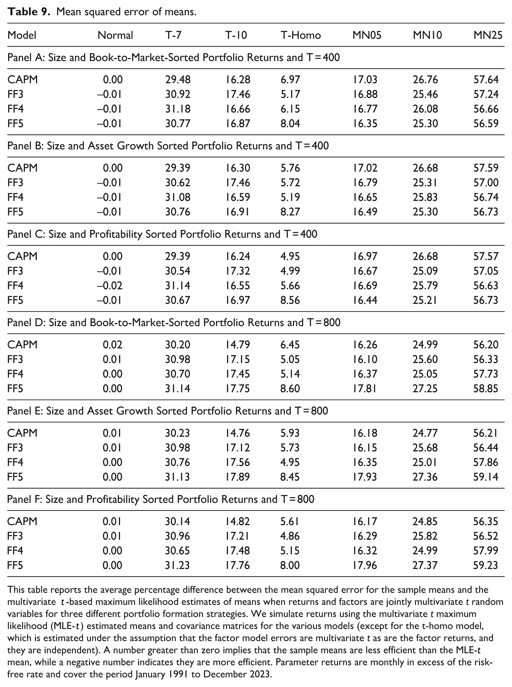
This table reports the average percentage difference between the mean squared error for the sample means and the multivariate t-based maximum likelihood estimates of means when returns and factors are jointly multivariate t random variables for three different portfolio formation strategies. We simulate returns using the multivariate t maximum likelihood (MLE-t) estimated means and covariance matrices for the various models (except for the t-homo model, which is estimated under the assumption that the factor model errors are multivariate t as are the factor returns, and they are independent). A number greater than zero implies that the sample means are less efficient than the MLE-t mean, while a negative number indicates they are more efficient. Parameter returns are monthly in excess of the risk-free rate and cover the period January 1991 to December 2023.

Table 10.

Mean squared errors of alphas.

Model	Normal	T-7	T-10	T-Homo	MN05	MN10	MN25
Panel A: Size and Book-to-Market-Sorted Portfolio Returns and T = 400
CAPM	-0.01	29.31	16.47	14.55	17.01	26.12	56.54
FF3	-0.01	29.31	16.65	15.90	17.58	26.42	56.44
FF4	-0.01	31.72	16.85	13.12	20.55	29.26	57.95
FF5	-0.01	31.76	17.22	13.77	20.82	29.45	57.26
Panel B: Size and Asset Growth Sorted Portfolio Returns and T = 400
CAPM	-0.01	29.14	16.34	14.51	17.34	26.39	56.80
FF3	-0.01	29.63	16.93	14.36	18.16	26.76	56.94
FF4	-0.01	31.41	17.22	15.35	20.60	29.05	57.44
FF5	-0.01	31.89	17.03	14.84	20.85	29.97	58.30
Panel C: Size and Profitability Sorted Portfolio Returns and T = 400
CAPM	-0.01	29.39	16.36	11.61	17.22	26.14	56.60
FF3	-0.01	29.88	16.68	12.24	18.08	27.01	57.14
FF4	-0.01	31.30	17.10	13.15	20.34	29.03	57.14
FF5	-0.01	31.93	16.97	12.62	21.21	30.07	57.67
Panel D: Size and Book-to-Market-Sorted Portfolio Returns and T = 800
CAPM	0.00	30.53	16.30	14.89	17.63	27.34	58.44
FF3	0.00	29.89	16.75	16.31	18.12	26.91	57.56
FF4	0.00	31.78	17.78	13.50	20.78	29.34	58.11
FF5	0.00	32.13	17.43	13.74	21.91	30.80	58.94
Panel E: Size and Asset Growth Sorted Portfolio Returns and T = 800
CAPM	0.00	30.73	16.47	15.17	18.11	27.67	58.65
FF3	0.00	30.16	16.88	14.51	18.72	27.49	58.04
FF4	0.00	31.76	17.68	16.34	20.61	29.39	58.06
FF5	0.00	32.25	17.23	15.23	22.04	31.15	59.12
Panel F: Size and Profitability Sorted Portfolio Returns and T = 800
CAPM	0.00	30.47	16.21	12.51	18.19	27.75	58.52
FF3	0.00	30.36	16.78	12.64	18.42	27.38	57.58
FF4	0.00	32.17	17.72	13.69	21.25	29.92	58.36
FF5	0.00	32.34	17.49	13.03	22.49	31.59	59.57

This table reports the average percentage difference between the mean squared error for the sample alphas and the multivariate t-based maximum likelihood estimates of alphas when returns and factors are jointly multivariate t random variables for three different portfolio formation strategies. We simulate returns using the multivariate t maximum likelihood (MLE-t) estimated means and covariance matrices for the various models (except for the t-homo model, which is estimated under the assumption that the factor model errors are multivariate t as are the factor returns, and they are independent). A number greater than zero implies that the OLS alphas are less efficient than the MLE-t alphas, while a negative number indicates they are more efficient. Parameter returns are monthly in excess of the risk-free rate and cover the period January 1991 to December 2023.

The multivariate t error model has regression errors distributed as multivariate t independent of f_t and is estimated using the EM algorithm outlined in Appendix B and simulated as discussed in Appendix D.

The mixture of normal distribution, in which X_t ~ N(μ,V₁) with probability p and X_t ~ N(μ,V₂) with probability 1 − p, is an elliptical distribution (as is the multivariate t) that exhibits fat tails. However, it is interesting to consider because in this case, the multivariate t distribution is misspecified, and yet the maximum likelihood estimates based on it may outperform the sample average because it is robust and downweights extreme returns. To keep parameterization manageable, we introduce a single parameter γ (that depends on p) and let V₁ = γ/(1 + p(1 − γ))V and V₂ = γ/(1 + p(1 − γ))V, so that, coupled with the fact that the means are state-invariant, the covariance matrix of X_t is V = pV₁ + (1 − p)V₂ since pγ/(1 + p(1 − γ)) + (1 − p)/(1 + p(1 − γ)) = 1. To ensure the kurtosis of the variables is plausible, we consider 3 cases: p_A = 0.005 and γ_A = 6.2981, p_B = 0.10 with γ_B = 5.3738, and p_C = 0.25 and γ_A = 5.4575. Appendix D describes how we simulate returns in all these cases.

Table 9 reports the average percentage increase in mean squared error across the mean parameters for the six models considered above, with two different sample sizes: 400 observations consistent with our current sample size, and 800, corresponding to a little over 66 years of monthly returns. When returns are normal, the robust multivariate t-based maximum likelihood estimator of the means performs about as well as the optimal ordinary least squares estimator. However, the multivariate t-based maximum likelihood estimator performs better than the least squares whenever there is excess kurtosis relative to the normal distribution, such as when returns and factors are jointly multivariate t random variables, when the factor model errors are multivariate t independent of the factors, or when returns and factors come from a fat-tailed distribution other than the multivariate t distribution. When the multivariate t distribution with 7 degrees of freedom, the sample mean has, on average, a MSE 30% higher, and when the degree of freedom is 10, the gains drop to about 17% when using 400 monthly observations and 15% when the sample size is doubled to 800. The T-Homo results refer to the homoscedastic multivariate t error model considered above. This model has returns with fat tails, but the heteroscedastic error joint multivariate t maximum likelihood estimator is misspecified. However, the sample average returns have an MSE that is still on average 5% larger than the (misspecified) maximum likelihood-based estimator. Finally, when we simulate returns from any of the three mixture of normal distributions that are elliptical random variables that exhibit excess kurtosis and produce heteroscedastic factor model errors but are not from the multivariate t distribution so the t-based maximum likelihood estimators are inefficient, but provide impressive improvements over the sample mean that on average have MSEs larger than our robust estimator of between 16% and 60% depending on parameterizations. This provides strong evidence that the MLE-t estimator is a useful robust estimator: even when returns are normal is doesn’t markedly underperform the optimal sample average because the normal case is a special case of the robust estimator when the degree of freedom parameter increases without bound. The only downside is one irrelevant parameter. However, when there are fat tails, even when these are drawn from a different distribution, and even when the factor model errors are homoscedastic, the robust multivariate t-based maximum likelihood estimator dramatically outperforms the sample average return. Table 10 repeats the experiment for alphas, and the same picture emerges: the robust multivariate t-based maximum likelihood estimator does no worse than the least-squares estimator when that is optimal and provides significant efficiency gains when returns exhibit fat tails, even when the multivariate t distribution is misspecified.

7. Conclusion

We explore the impact of relaxing the normality assumption and estimate means, alphas, and betas using methods other than least squares. We provide strong evidence against the multivariate normality assumption using tests of multivariate skewness and kurtosis, but we cannot reject the null hypothesis that returns and factors are jointly multivariate t random variables with 7 degrees of freedom. This approach is different from the case where the multivariate regressions are estimated assuming that the residuals are multivariate t conditional on the factors, which means that the residuals are conditionally heteroscedastic.

Although estimates of standard deviations and betas are similar when returns are estimated using maximum likelihood under normality and the multivariate t distribution, estimates of means and alphas change dramatically. We find that the mean excess return for the small growth portfolio decreases by more than 0.8% per month, the mean estimate of the size SMB factor flips from positive to negative, and the average squared alphas are typically higher after accounting for fat tails. The evidence against asset pricing models are higher using the likelihood ratio test under the multivariate t distribution than under the normal, showing the importance of accounting for non-normality.

Key practical and research applications

• Extreme returns are common stock returns, and traditional estimates of key features of asset pricing models, such as the price of factor risk, are adversely affected by such outliers.

• Estimating models using robust measures provides practitioners with more reliable parameter estimates. Simulation results show that the robust estimation method based on the multivariate t distribution performs much better even when returns have extreme returns from a range of fat-tailed distributions, and it shows that the sign of the size effect changes relative to the sample average factor return.

• The robust methods provide practitioners and researchers alike with improved estimation tools.