Sage Journals: Discover world-class research

Abstract

COVID-19 has had a significant economic impact on Australia, and consequently on the superannuation savings of many individuals. To examine COVID-19’s heterogeneous effects across different industries and demographic groups, the impact on superannuation was assessed for 12 representative cameos using a range of Australian data, including Household, Income and Labour Dynamics in Australia (HILDA), ATO, ABS and APRA sources. The marginal impacts of sudden job loss, investment losses, investment switching and participation in the Early Release of Superannuation (ERS) scheme were each investigated in turn. The cameos highlight that some demographic cohorts faced several compounding challenges. For example, many ERS applicants were already facing financial hardship, were more likely to be younger, and faced a higher risk of unemployment. This highlights that COVID-19 has impacted different cohorts in different ways, depending on age, employment status and industry, and family situation, among other factors.

JEL Classification: D14, D15, J26, J32

Keywords

COVID superannuation retirement

1. Introduction

Though primarily a public health issue, the economic impacts of COVID-19 have also been significant (RBA, 2020b). The implementation of border closures, social distancing measures and lockdowns restricted movement and disrupted labour markets (ABS, 2021a). The superannuation savings of Australians were also significantly impacted, for a range of reasons. A sharp rise in unemployment in some industries gave rise to a reduction in superannuation contributions in the short term. Immediate investment losses were compounded by many members’ decisions to switch to cash investment options. Indeed, there was a 1.5% increase in cash assets in March 2020, a larger movement than during the Global Financial Crisis where member switching flows were relatively small (Gerrans, 2012; Mercer, 2020; RBA, 2021a). Members who switched to cash forwent the subsequent market recovery, and losses also crystallised for those who withdrew superannuation sums under the Early Release of Superannuation (ERS) scheme (RBA, 2021a; Wherrett et al., 2021).

Notably, these impacts were not homogeneous across the population (Salt, 2021). Unemployment was concentrated in particular industries such as hospitality, retail and entertainment, which generally had low- and middle-income earners, a casual workforce and high female representation (Australian Unions, 2020; Hodgson, 2020; Mercer, 2020). Unemployment was also high for younger age groups (ABS, 2021b), but also brought on early retirement for others due to fewer employment opportunities (Mercer, 2020).

A temporary ERS policy was announced, allowing those with adverse financial circumstances the ability to withdraw up to an untaxed $10,000 from their superannuation in each of the 2019–2020 and 2020–2021 financial years. High rates of ERS withdrawals occurred for those working in industries impacted by COVID-19 and who were therefore also exposed to greater risks of unemployment, with concentrated impacts in certain regions and age groups (ASFA, 2020b; The Treasury, 2020b). As such, some industry superannuation funds experienced higher levels of ERS withdrawals than others, with several smaller funds compelled to release more than 10% of funds under management (FUM) (ASFA, 2021). Several funds experienced a significant increase in cash assets (exceeding 3% of FUM, twice the industry average), with older members and those with larger superannuation balances more likely to switch to cash (RBA, 2021a).

Some demographics were prone to facing a number of impacts in combination, compounding their effect(s). For example, a large portion of ERS applicants had likely already faced financial hardship during the pandemic, were more likely to be younger, and faced a higher risk of unemployment. Recent commentary has also highlighted delays in returning to work for ERS participants (McIlroy, 2022). Those approaching retirement were exposed and less able to absorb sustained market losses, and for younger cohorts, losses will be compounded over time.

The effects on long-term savings arising from shocks such as that associated with COVID-19 are not yet fully understood. Some short-term impacts and features of the ERS have been studied, such as Wang-Ly and Newell (2022) who found that the ERS was successful in providing immediate financial support to those in need. In addition, Bateman et al. (2023) found significant heterogeneity in ERS participants’ decision-making processes, with many people either mis-estimating or not estimating how a withdrawal could ultimately impact on their retirement savings in the longer term.

This study contributes to the existing literature by providing estimates of long-term rather than short-term impacts on superannuation. It considers how COVID-19 has impacted combinations of factors that are relevant to superannuation savings and examines the heterogeneous nature of such impacts across different cohorts of the population. This in turn highlights the role(s) of both superannuation funds and the financial advice industry in responding to such crises, and consequently, in how to best help people navigate a post-COVID pathway to financial provision in retirement. It also increases the understanding of the consequences of future economic shocks, if similar policy responses are required.

The remainder of this article is arranged as follows. Section 2 provides the background that motivated this study. Section 3 describes the data and methodology. Section 4 discusses the results of the projections. Section 5 discusses the implications of our findings, and Section 6 concludes.

2. Background

2.1. Superannuation and retirement

In Australia, individuals derive an income in retirement through three main sources: first, a publicly funded and means-tested Age Pension; second, a compulsory and tax-advantaged superannuation savings scheme; and third, personal savings (including home ownership). The Age Pension is generally the main source of income for those with moderate levels of wealth (The Treasury, 2020b). Under compulsory superannuation, employers are currently required to pay 11% (increasing to 12% by July 2025) of an employee’s earnings into the employee’s superannuation fund (ATO, 2021). By 2040, most retiring employees will have had superannuation contributions of at least 9% for most of their working life (Lamarra et al., 2022).

However, a gender gap in retirement savings also exists (Knox et al., 2021). This is largely driven by employment outcomes, with females having longer periods out of the workforce due to caring duties, greater propensity to work part-time, and lower average wages in female-dominated industries such as health, education and hospitality (Dawson and Casey, 2020; Knox et al., 2021; The Treasury, 2020b). Furthermore, while promotions typically happen between the ages of 25 and 40, this is also when women have and raise children (Knox et al., 2021).

In general, individuals cannot access their superannuation savings until age 60 (for those born after 1964). However, earlier access to superannuation is possible in some circumstances, including terminal illness, incapacity, compassionate grounds and severe financial hardship (ATO, 2023a). Since 2017, access has also been allowed to voluntary superannuation contributions for the purposes of helping the purchase of a first home (ATO, 2023b).

Notably, as superannuation savings have increased since first being made compulsory in 1992, employer-sponsored defined benefit (DB) schemes have declined. This has contributed to the individualisation of financial security in retirement, alongside the decline of traditional insurance products. Such individualisation increases the longevity, investment and inflation risks that individuals are exposed to (Lamarra et al., 2022). When combined with a complex financial system, and generally low levels of financial literacy to manage such risks (Lin et al., 2019), a better understanding of personal financial choices and well-being is important (Bruhn, 2015).

In this context, the COVID-19 pandemic provides a potentially long-lasting economic impact upon the lives of many. As such, an economic shock of the magnitude provided by COVID-19 is of some interest, to examine how it has impacted superannuation’s role as a central pillar of financial well-being in retirement.

2.2. COVID-19 and economic impacts

COVID-19 is a highly transmissible infectious disease caused by a form of coronavirus and was identified in late December 2019 (Department of Health, 2021; World Health Organization, 2020a). Australia registered its first case on 25 January 2020 (Storen and Corrigan, 2020), a public health emergency of international concern was declared by the World Health Organization on 30 January 2020, and COVID-19 was declared a pandemic on 11 March 2020 (World Health Organization, 2020b, 2020c).

Significant measures were introduced in Australia to prevent the spread of COVID-19, including social distancing and business restrictions (ABC News, 2020). Industries hardest hit by social distancing requirements were hospitality, retail and entertainment. Several states implemented border restrictions, and Australian borders were closed to non-residents, further impacting industries such as tourism and education (Hodgson, 2020; RBA, 2020a). As cases grew and spread across the world, the ensuing economic shock was severe. The RBA announced support for the banking system, reduced the cash rate target to a historic low of 0.25%, and undertook quantitative easing (RBA, 2020b). A range of additional government support was also implemented (Prime Minister of Australia, 2020).

The impacts on labour markets were significant. Seasonally adjusted unemployment reached a 10-year high by July 2020, with larger impacts in industries with greater numbers of lower- and middle-income earners (ABS, 2021b; Mercer, 2020), in states that implemented strict border and stay-at-home restrictions (ABS, 2021b), and among youth, particularly females (ABS, 2021b; Salt, 2021). Wage growth fell significantly, especially in accommodation and food services (ABS, 2020d). Gross domestic product (GDP) fell 0.3% in the March 2020 quarter and 7% in the June 2020 quarter, reflecting Australia’s first recession in 29 years (ABS, 2020d; RBA, 2021b).

As case numbers started to decline, stay-at-home and travel restrictions were relaxed. Unemployment fell to pre-pandemic rates in May 2021 (ABS, 2021b), and underemployment, labour participation and youth unemployment recovered somewhat, as did GDP growth (ABS, 2021d). However, Australia has since had further outbreaks of COVID-19 cases. While these have not led to an economic shock comparable to 2020, the long-term impacts of COVID-19 may not be fully mature.

2.3. Superannuation impacts and the ERS

Superannuation funds, with approximately 17 million members in Australia (ASFA, 2020a), were not immunised to the economic shocks from COVID-19. In March 2020 alone, the median balanced superannuation fund fell 8.9%, and the median growth superannuation fund fell 12.5% (Robertson, 2020).

In order to provide immediate funds for those faced with sudden job loss and/or other adverse financial circumstances, a temporary ERS policy was announced. This allowed people to withdraw up to $10,000 (untaxed) from their superannuation in each of the 2019–2020 and 2020–2021 financial years. Various eligibility criteria applied, including being unemployed, in receipt of a range of government benefits, or having working hours reduced, which overrode existing preservation rules (The Treasury, 2020a). As such, a large number of applicants were already facing financial distress. The rationale for the ERS was that access to immediate funds in a period of economic distress would have benefits in excess of preserving funds until retirement (The Treasury, 2020b).

ERS withdrawals occurred in two tranches, between April and June 2020, and July and December 2020. By January 2021, 4.8 million applications had been approved and $36.4 billion in funds had been paid (an average of $7638 per approved application) (APRA, 2021). Single parents and those with lower levels of education had the highest tendency to participate (Warren, 2021). Meeting immediate financial needs such as mortgage payments, rent or household bills were major reasons for participation, with approximately half of applicants citing a reduction in working hours, and a fifth being unemployed (ABS, 2020e; ATO, 2021; Baker and Daniel, 2020).

Significant liquidity challenges consequently arose for the Superannuation industry, with 2% of total FUM released in 2020 (RBA, 2021a). Withdrawals prior to the pandemic under existing early release criteria presented a diversifiable liquidity risk; in contrast, the ERS scheme prompted millions of withdrawal applications in a short period of time (RBA, 2021a). Elevated demand from members for low-risk rather than risky assets also contributed to liquidity challenges (Mercer, 2020; RBA, 2021a), as did the need to meet margin calls on hedges (RBA, 2021a). Of note is that the above factors occurred simultaneously, highlighting a vulnerability to risk aggregation. However, while ERS scheme recipients were generally young, those increasing their allocation to cash assets were typically closer to retirement (ASFA, 2021; Mercer, 2020).

Given the role of superannuation to provide retirement income, it is important to understand the impact of COVID upon the superannuation balances of different cohorts of Australians. In particular, it is evident in studies of ERS participants that people face challenges in balancing trade-offs between saving and spending over a lifetime (Bateman et al., 2023). Furthermore, although Wang-Ly and Newell (2022) highlight a positive impact on individuals’ financial well-being as a consequence of participation in the ERS, this is considered in only a short-term context. Therefore, we explore three key questions that complement prior studies. First, what is the long-term impact on superannuation savings arising from COVID-19; second, what is the long-term impact in meeting modest and comfortable levels of income in retirement; and third, how do these impacts between different cohorts in the population.

We therefore select a number of cohorts for analysis of the longer-term impact, to ascertain the heterogeneous nature of impacts across the population.

3. Methodology and data

To quantify the impacts of COVID-19 upon the superannuation savings for certain cohorts, a model simulating the experience of representative individuals was built. Assessing impacts across 12 representative individuals (cameos) rather than the aggregate population was chosen to highlight that impacts were not uniform, but were focussed on certain cohorts – particularly those who were eligible for ERS. An aggregate assessment would provide a measure of materiality across the population, but would also dilute insights about consequences of COVID-19 on vulnerable cohorts. The use of cameos assists the focus on these cohorts, in a similar manner to studies that consider superannuation and retirement well-being (e.g. Butt et al., 2022). Outcomes from 2020 to retirement were simulated 1000 times for each selected cameo, for a hypothetical ‘COVID-free’ scenario (Part A) in order to estimate a counterfactual case, and then for a scenario incorporating the impacts of COVID-19 (Part B).

One metric used to examine the impact of COVID-19 included the difference in projected superannuation balances at retirement. To examine adequacy of retirement income, various benchmarks exist. ASFA offers a retirement income metric through categorising ‘modest’ and ‘comfortable’ living standards, which quantify the aggregated cost of common expenditure items such as household, transport and health expenses, for both singles and couples, in two age ranges. These provide a benchmark that help assess the impact of COVID-19 on retirement living standards. As such, another metric is the simulated probability of exceeding these living standards benchmarks. An analysis of change was also conducted to assess the drivers in differences between Part A and B outputs.

Model characteristics included age, age of retirement, gender, employment status (both at the beginning and end of the 2019–2020 financial year), starting superannuation balance, any ERS withdrawn, and whether superannuation was moved into cash assets. Changes in marital status, years that any children were born and highest level of education were also factored into projections, as these influence an individual’s employment, income and future superannuation. The key variables of employment status, taxable income, superannuation (investment) returns and fees, and wage growth are each discussed in turn below, following a description of the main data sources used for the model.

3.1. Data sources

Waves 14 to 19 of the Household, Income and Labour Dynamics in Australia (HILDA) Survey were used as a longitudinal guide of labour status transition and hourly wage regression estimates, as well as distributions of hours worked per week. Characteristics such as age and employment status were informed by summary statistics of ERS applications received during 2020 (ATO, 2021). Historical wage growth was sourced from the Wage Price Index (WPI) published by the Australian Bureau of Statistics (ABS, 2020a; 2020b; 2020c). Past investment performance and fees were used from 9 of the largest 10 superannuation funds in Australia¹ to construct fund distributional assumptions. Further characteristics were informed by application data released by Treasury and survey data conducted by the Australian Institute of Family Studies.

3.2. Modelling approach

To incorporate more realism than a static model, the constructed model was dynamic, where variables such as employment status, hourly wages and superannuation balance each year were functions of endogenous variables in previous years. The model incorporated multiple stochastic processes, such as wage growth, superannuation fund investment returns and hours worked. Monte Carlo simulations were conducted to establish a representative distribution of outcomes, which also allowed estimates of confidence levels of exceeding ASFA living standards benchmarks. This improves on a deterministic model, where unexplained variability would not be incorporated and only a point estimate would be computed (Britton et al., 2019; Higgins and Sinning, 2013).

The approach to model labour force transitions, hourly wage, hours worked, wage growth and superannuation returns and fees are each discussed in the following sections.

3.2.1. Labour force transitions

Three logistic regression models were built using HILDA data to estimate the probability of being in each of four labour force states in a given year. The first logistic regression model determined the probability of being employed. The second determined the probability of working full-time (FT) or part-time (PT), conditional on being employed. The third model quantified the probability of being unemployed or not in the labour force (NILF), conditional on not being employed. The equations for the three models are as follows, with random variable $Y_{i t}$ the bivariate choice of individual $i$ at time $t$ , $β$ a vector of coefficients and $X$ a vector of observed covariates (Higgins and Sinning, 2013)

P (Y_{i t}^{a} = k | X_{i t}^{a}) = \frac{\exp (β_{k}^{a} X_{i t}^{a})}{1 + \exp (β_{k}^{a} X_{i t}^{a})}

(1)

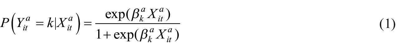
where $k = 0$ (not employed), 1 (employed)

P (Y_{i t}^{b} = k | X_{i t}^{b}) = \frac{\exp (β_{k}^{b} X_{i t}^{b})}{1 + \exp (β_{k}^{b} X_{i t}^{b})}

(2)

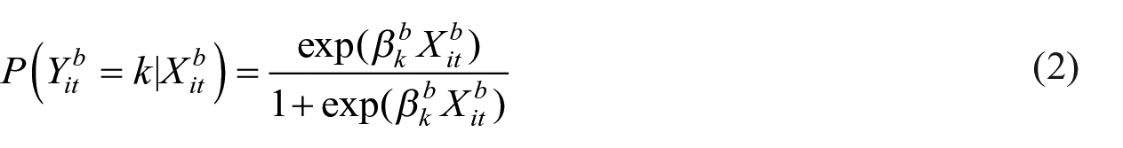
where $k = 0$ (PT), 1 (FT)

P (Y_{i t}^{c} = k | X_{i t}^{c}) = \frac{\exp (β_{k}^{c} X_{i t}^{c})}{1 + \exp (β_{k}^{c} X_{i t}^{c})}

(3)

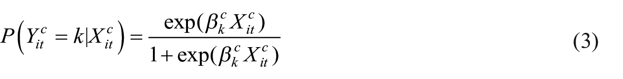
where $k = 0$ (NILF), 1 (unemployed).

The transitions were evaluated by reconciling cumulative probabilities across discrete employment states with a uniform randomly drawn number between 0 and 1 for a given year and simulation. Of note is that different individual characteristics infer differing propensities to be in each labour force state at different stages of life (Higgins and Sinning, 2013). Significant indicators of labour force status included age, gender, employment status in the previous 5 years, highest level of education, relationship status and age of youngest child. Interactions between age and marital status, gender and age of youngest child, and gender and marital status were also fitted. These are standard covariates used in labour force models (Haynes et al., 2006; Higgins and Sinning, 2013).

A cubic spline was used to fit curves on the propensities of being in each employment state across age, to address the non-linear association between labour force status and age. Cubic splines allowed for fluctuations in employment propensities across ages to be more effectively captured in the model than by categorising ages into groups, while minimising the number of parameters fitted. The number of knots chosen in this cubic was tuned and determined based on comparisons of Akaike information criterion (AIC). The movements in employment propensities across ages differed significantly by gender, justifying the employment of a cubic spline for age as well as an interaction term between age and gender. Five variables representing the previous 5 years of employment states were included with the four labour force states as categories. This allowed the model to be a fifth-order Markov process, with a more complex employment status serial dependency structure. Education categories were year 11 and below, year 12, certificate or tertiary diploma, and bachelor’s degree or higher. Relationship status had categories never married, legally married or de facto, separated, divorced or widowed. Age of youngest child was fitted as a categorical variable rather than a cubic spline, given that nearly 70% of the observations in the HILDA data used for modelling did not have a child under the age of 14. Categories for age of youngest child for people with a child included 0, 1, 2 to 5, 6 to 10 and 10 to 14. These age boundaries were chosen based on the observed movements in employment state propensities across youngest child ages, particularly for females with a young child. The interaction term of youngest child’s age and gender was included given the contrasting employment propensities across genders (higher comparative FT employment for fathers with a baby, while nearly half of mothers with a newborn were NILF). Other predictors such as number of children were explored but were not evaluated to be a significant addition to the model given its connection to age of youngest child, with model parsimony also an important consideration. Other interaction terms were tested and eliminated by comparing AIC.

3.2.2. Hourly wage

Rather than treating weekly earnings as a single variable, hourly wage is more suitable to apply across all employment states and is then combined with hours worked per week. Although copula functions can be employed to represent year-to-year dependency (Britton et al., 2020), a regression model was used to more simply cater for multiple non-binary or continuous covariates that may influence income and include previous years’ variables such as employment status.

Six years of HILDA data was used, with hourly wages inflated to 2019–2020 dollars. Given that individuals appear in multiple HILDA waves, they are represented multiple times in the model, to incorporate transitory variation and permanent differences (Higgins and Sinning, 2013). Hourly wage observations below $5 and above $150 were removed, as were ages below 23 or above 64 years. Due to sparsity of observations between 65 and 67, estimated wages for those aged 64 were used.

An ordinary least squares regression was fit with the natural logarithm of hourly wages set as the dependent variable. This model featured some predictors identical to that in the labour force logistic regression: gender, marital status, education and a cubic spline fitted for age. Age of youngest child had categories of no child, 0 to 5, and 6 to 14, with lower variability of average wage compared to labour state propensities. Current labour force status was included, as were terms interacting age with other predictors such as gender, age of youngest child, education and employment status (and selected through comparing AIC between candidate models).

Previous year’s hourly wage was not included, with serial dependence addressed through transitory variation and permanent differences (Higgins and Sinning, 2013). Permanent differences, denoted $u_{i t}$ for cameo $i$ at time $t,$ capture the difference between the predicted logarithm of hourly wage and the logarithm of hourly wage within HILDA. Permanent components featured an independent and identically distributed annual random shock, denoted $w_{i t},$ to reflect that observed residual variances and covariances increase with age. This is therefore modelled as a random walk. Transitory variation, denoted $v_{i t},$ was incorporated to capture differences due to other reasons.

The hourly wage model, with $β$ a vector of coefficients and $X$ a vector of observed covariates, can be expressed as follows (Higgins, 2011)

\log (W_{i t}) = β X_{i t} + u_{i t} + υ_{i t}

(4)

u_{i t} = u_{i, t - 1} + w_{i t}

3.2.3. Hours worked per week

Distributions of hours worked were constructed using HILDA data, characterised by employment status, gender and (for PT employment) whether the individual had a child under the age of 6 (in line with Higgins and Sinning, 2013). No further covariates of hours worked were modelled.

Hours worked per week was modelled to remain unchanged across years if the simulated employment state remained unchanged. Where labour force movement occurred, hours worked was simulated by applying the inverse transformation algorithm to the relevant hours worked probability mass function.

3.2.4. Wage growth

Wage growth was modelled by fitting a moving average time series model on historical WPI data. WPI is unaffected by compositional labour force changes, employee characteristics and hours worked, and is not uniform across industries or location (ABS, 2021c; The Treasury, 2017). However, given occupation and location were not modelled, an overall WPI was modelled for each cameo. Although drivers of wage growth include age, education and employment contract (Kalb and Meekes, 2020), these were addressed in the hourly wage regression model.

Although wage growth is also a function of labour market capacity and inflation expectations (Andrews et al., 2019), these were not estimated in the model. CPI is historically more volatile than WPI, with WPI also exhibiting serial correlation, justifying the use of an autoregressive integrated moving average (ARIMA) time series model. A moving average process was an intuitive model fit, based on the historical semi-annual wage growth data. A moving average process of order 2 (MA(2)) model produced a lower AIC than other associated ARIMA processes and was defined as

X_{t} - X_{t - 2} = e_{t} + β_{1} e_{t - 1} + β_{2} e_{t - 2}

(5)

$X_{t}$ whereis the semi-annual wage growth at time $t;$ $X_{t - 2}$ is the semi-annual wage growth 2 six-month periods or 1 year earlier; $e_{t}$ is a white noise process, assumed to be normally distributed with variance $σ^{2}$ ; with $e_{t - 1}$ and $e_{t - 2}$ the forecast errors at time $t - 1$ and $t - 2,$ respectively.

The standard deviation of the white noise process was estimated as 0.244%.

Wage growth at time $t$ was projected by simulating the white noise process $e_{t}$ and using previous white noise process values $e_{t - 1}$ and $e_{t - 2},$ subject to a minimum wage growth of 0. Wage growth was simulated from 2019 to 2020 for Part A and from 2021 to 2022 for Part B.

For the financial year ending at time $t,$ annual wage growth ( $Y_{t}$ ) was therefore calculated through combining two semi-annual growth rates as follows

Y_{t} = (1 + X_{t - 1}) (1 + X_{t}) - 1

(6)

where $X_{t - 1}$ and $X_{t}$ are semi-annual wage growth amounts for the 6 months ending at time $t - 1$ and $t,$ respectively, with each increment of time representing 6 months.

Modelled wage growth was also used as a discount rate, to provide present value estimations of retirement balances in the future. This choice of deflator is consistent with that used by The Treasury (2020b) for periods up until retirement age.

3.2.5. Superannuation returns and fees

A historical superannuation returns series was established by calculating the average annual return, weighted by total assets, across the balanced fund investment options of nine sampled funds (constituting 62% of total MySuper assets at 30 June 2020). This series did not display significant temporal dependency and was not correlated to WPI or CPI. A Weibull distribution fitted on a linear transformation of superannuation returns produced the lowest AIC of candidate probability distributions, reflecting the negative skewness of the average returns data. This gave an expected return of 7.6%, a standard deviation of 10.1%, and a 13.8% probability of a negative return in a given year. To differentiate the COVID-19 scenarios, superannuation returns were simulated from 2019 to 2020 for Part A and 2021 to 2022 for Part B (the latter to incorporate observed returns in 2019–2020 and 2020–2021). Cash investment returns in 2020–2021 captured the investment switch response to declining equities in March 2020.

Estimates of fixed and percentage of FUM fees were the weighted average of the superannuation funds’ fees. The fixed component was increased by wage growth over time.

3.3. Cameo selection

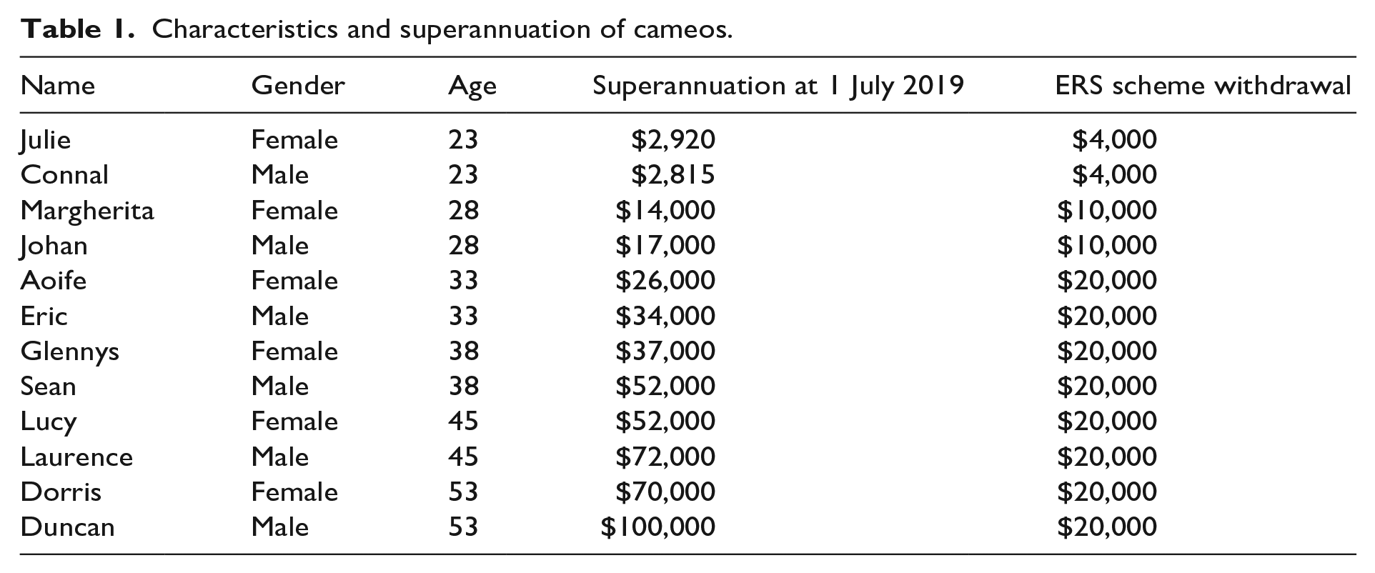
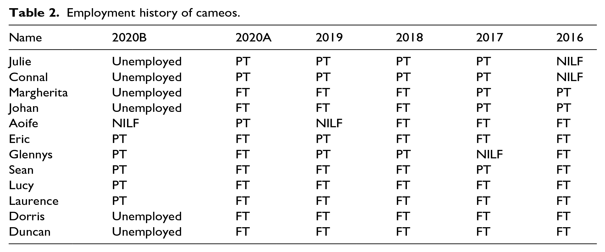
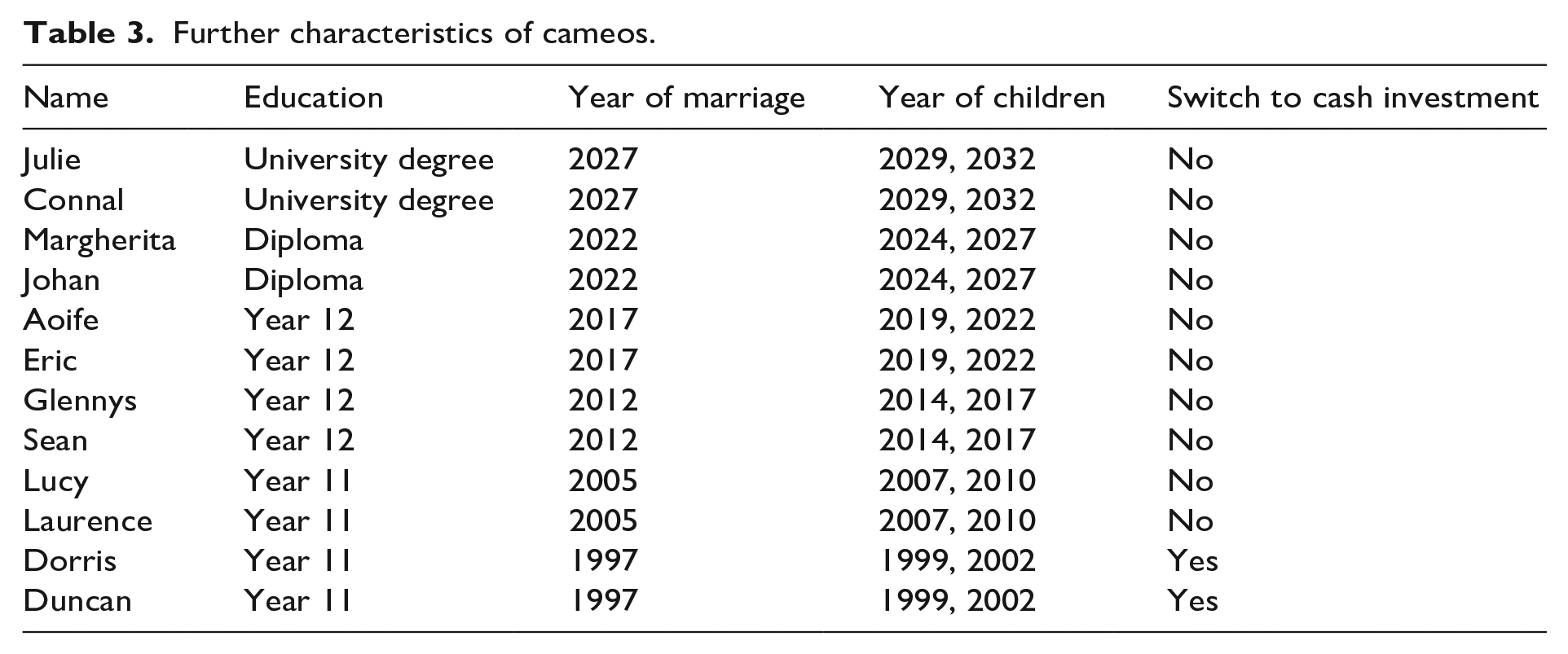
Male and female cameos were explored across six different ages. While males made up approximately 56% of all approved ERS scheme applications (ATO, 2021), an equal number of male and female cameos were constructed to provide a gender comparison. Superannuation balances and ERS scheme withdrawals were subsequently tailored on age and gender profiles. Each cameo was associated with a name rather than a number or other identifier, as a style choice to personalise the modelling of that cameo. Tables 1 to 3 detail the characteristics chosen for each of the resultant 12 cameos.

Table 1.

Characteristics and superannuation of cameos.

Name	Gender	Age	Superannuation at 1 July 2019	ERS scheme withdrawal
Julie	Female	23	$2,920	$4,000
Connal	Male	23	$2,815	$4,000
Margherita	Female	28	$14,000	$10,000
Johan	Male	28	$17,000	$10,000
Aoife	Female	33	$26,000	$20,000
Eric	Male	33	$34,000	$20,000
Glennys	Female	38	$37,000	$20,000
Sean	Male	38	$52,000	$20,000
Lucy	Female	45	$52,000	$20,000
Laurence	Male	45	$72,000	$20,000
Dorris	Female	53	$70,000	$20,000
Duncan	Male	53	$100,000	$20,000

Table 2.

Employment history of cameos.

Name	2020B	2020A	2019	2018	2017	2016
Julie	Unemployed	PT	PT	PT	PT	NILF
Connal	Unemployed	PT	PT	PT	PT	NILF
Margherita	Unemployed	FT	FT	FT	PT	PT
Johan	Unemployed	FT	FT	FT	PT	PT
Aoife	NILF	PT	NILF	FT	FT	FT
Eric	PT	FT	PT	FT	FT	FT
Glennys	PT	FT	PT	PT	NILF	FT
Sean	PT	FT	FT	FT	PT	FT
Lucy	PT	FT	FT	FT	FT	FT
Laurence	PT	FT	FT	FT	FT	FT
Dorris	Unemployed	FT	FT	FT	FT	FT
Duncan	Unemployed	FT	FT	FT	FT	FT

Table 3.

Further characteristics of cameos.

Name	Education	Year of marriage	Year of children	Switch to cash investment
Julie	University degree	2027	2029, 2032	No
Connal	University degree	2027	2029, 2032	No
Margherita	Diploma	2022	2024, 2027	No
Johan	Diploma	2022	2024, 2027	No
Aoife	Year 12	2017	2019, 2022	No
Eric	Year 12	2017	2019, 2022	No
Glennys	Year 12	2012	2014, 2017	No
Sean	Year 12	2012	2014, 2017	No
Lucy	Year 11	2005	2007, 2010	No
Laurence	Year 11	2005	2007, 2010	No
Dorris	Year 11	1997	1999, 2002	Yes
Duncan	Year 11	1997	1999, 2002	Yes

The following insights on ERS composition is informed by the ATO (2021):

• Approximately 10% of ERS applicants were aged 25 and under. This age group generally has modest superannuation balances, with a balance of $4000 assumed for both genders, which is fully withdrawn under the ERS. This is consistent with the large numbers of those aged under 35 who withdrew their entire superannuation balance between April and June 2020 (Industry Super Australia, 2020).

• Approximately 16% of ERS applicants were aged between 26 and 30. Superannuation balances could cover a $10,000 withdrawal in the first tranche, but not a second. This aligns with survey data that found that 74% of male applicants and 81% of female applicants under 30 withdrew $10,000 or less across both tranches (Warren, 2021). The male cameo commenced with a higher superannuation balance, with the gender difference aligning with Dawson and Casey (2020).

• Approximately 17% of ERS applicants were aged between 31 and 35. Those in this group were more likely to be able to withdraw the full $20,000. A greater gender difference in superannuation balances exists compared to younger cameos, consistent with Hodgson (2020), although both genders can make a full ERS withdrawal of $20,000. Nearly 50% of ERS applicants applied in both financial years, with a mean single withdrawal amount of approximately $8200. With more than a quarter of applicants aged 30 or younger, who are less likely to be able to make maximum withdrawals, all cameos over the age of 30 were therefore assumed to withdrawal the maximum amount of $20,000.

• The ages of 38, 45 and 53 represented groups aged from 36 to 40, 41 to 50 and 51 to 55, who made up 15%, 23% and 9% of all ERS applications, respectively. Cameos for these ages all withdrew the maximum amount of $20,000.

Other characteristics such as employment history, education, children and partner status were chosen based on the age of each cameo and adjusted to determine the role they each play on each cameo’s impact of COVID-19. These are given below.

Given the lack of ERS cross-sectional data, nominal retirement balances of each cameo at retirement age are not scrutinised in detail. Instead, differences between a COVID-free scenario and a COVID scenario are examined. For simplicity, ASFA’s stated superannuation balances required to achieve benchmark retirement incomes (allowing for a part or full age pension) were the basis to assess sufficiency of achieving a modest or comfortable retirement income (ASFA, 2018). This obviated the need for detailed assumptions about how assets were consumed in retirement, as the focus was on the impact of COVID-19 on projected superannuation balances at retirement.

4. Results

Results are presented in three main sections. First, the impact on projected retirement balances, then a deeper analysis of change/drivers of these differences, and then the impact on retirement incomes. We then present some insights around the age pension, and the gender gap in financial outcomes. The findings of selected sensitivity analyses are then also presented.

4.1. Superannuation at retirement

The impact on the modelled cameos were varied and align with the heterogeneous impacts of COVID-19 on the labour force, wage growth, ERS withdrawals and switches to cash investments.

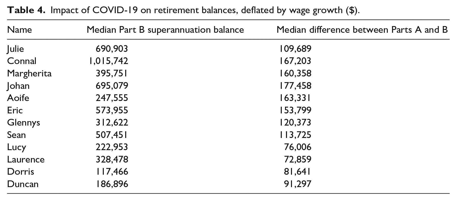
Of all cameos, 28-year-old Johan had the highest median fall in superannuation balance at retirement. There are various reasons why this has occurred. First, with nearly 40 years until retirement, the impacts of COVID-19 have a long time to compound, relative to older cameos. Second, Johan had a higher superannuation balance to withdraw from than other younger cameos. Third, he went from FT work to unemployment, hence suffered a larger labour force shock than several others. Furthermore, as his modelled income earning potential is high given his qualification and gender, his foregone income in 2020 was larger than some others as well. Other cameos such as Connal, Margherita, Aoife and Eric had impacts of similar magnitude, but each driven by differing causes.

Laurence and Lucy had the smallest impact. Both were aged 45 and faced reduced work hours, leading to a withdrawal of $20,000 of superannuation. However, with no job loss and a shorter time to retirement, this dampened the impact of low wage growth and compounding returns, compared to younger cameos.

Table 4.

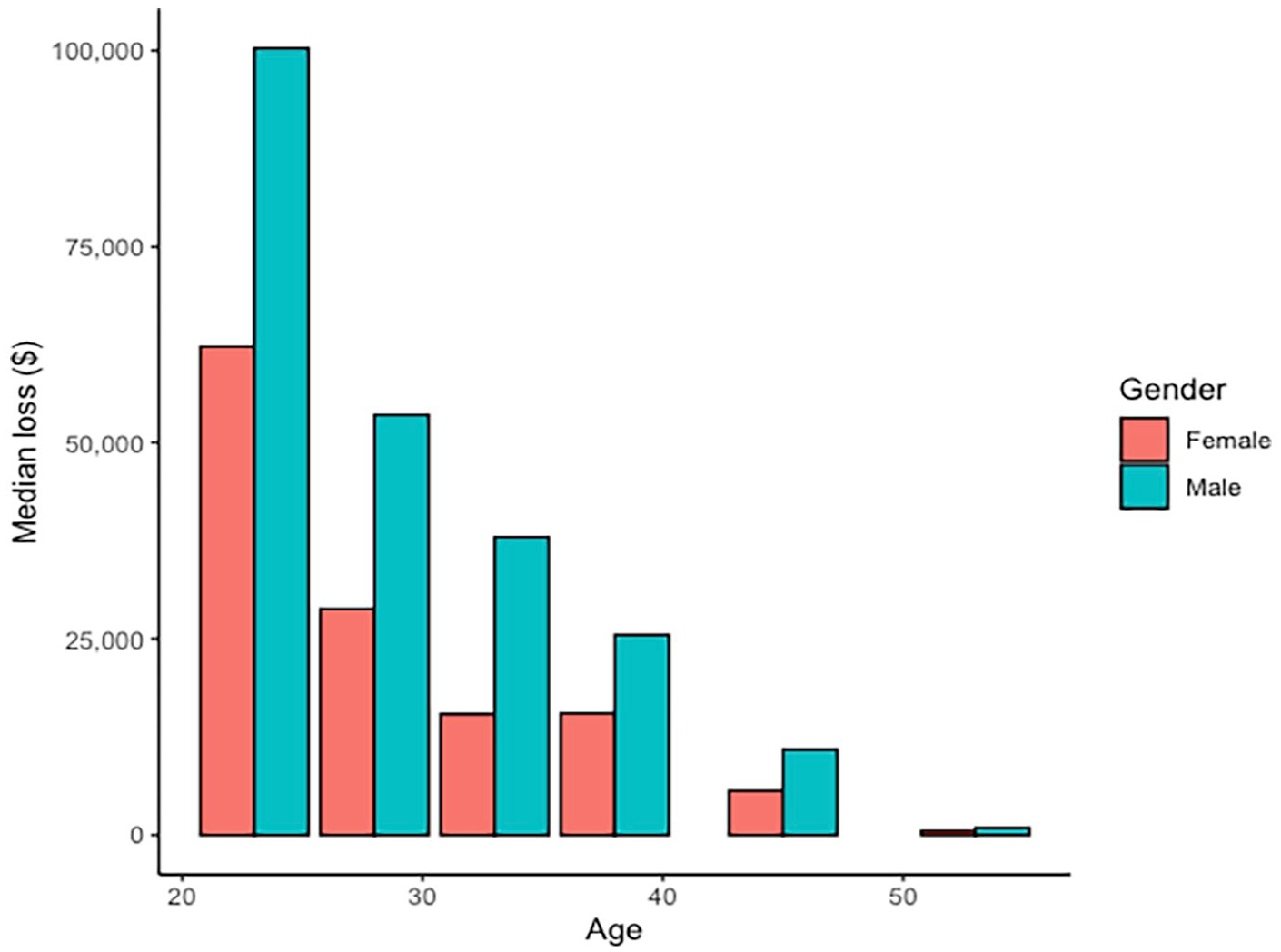
Impact of COVID-19 on retirement balances, deflated by wage growth ($).

Name	Median Part B superannuation balance	Median difference between Parts A and B
Julie	690,903	109,689
Connal	1,015,742	167,203
Margherita	395,751	160,358
Johan	695,079	177,458
Aoife	247,555	163,331
Eric	573,955	153,799
Glennys	312,622	120,373
Sean	507,451	113,725
Lucy	222,953	76,006
Laurence	328,478	72,859
Dorris	117,466	81,641
Duncan	186,896	91,297

Table 5.

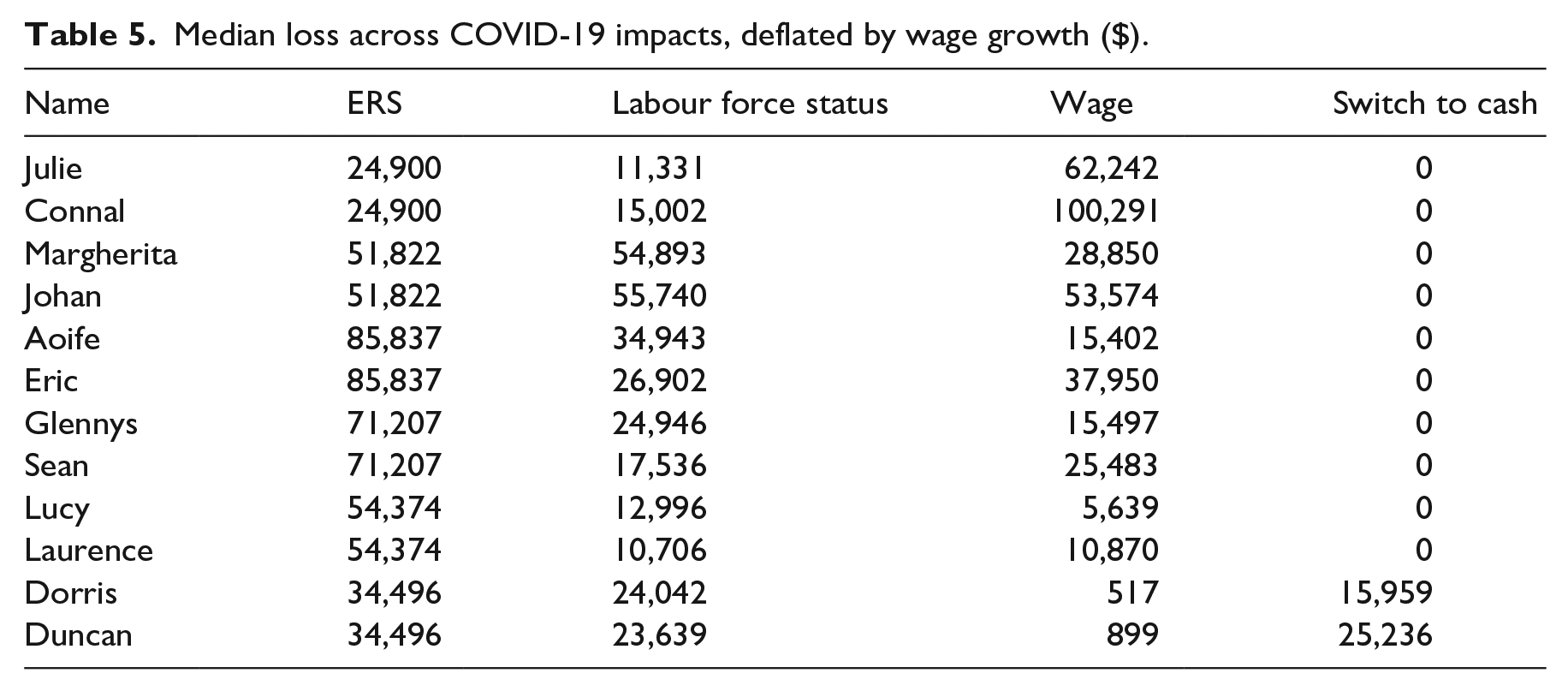
Median loss across COVID-19 impacts, deflated by wage growth ($).

Name	ERS	Labour force status	Wage	Switch to cash
Julie	24,900	11,331	62,242	0
Connal	24,900	15,002	100,291	0
Margherita	51,822	54,893	28,850	0
Johan	51,822	55,740	53,574	0
Aoife	85,837	34,943	15,402	0
Eric	85,837	26,902	37,950	0
Glennys	71,207	24,946	15,497	0
Sean	71,207	17,536	25,483	0
Lucy	54,374	12,996	5,639	0
Laurence	54,374	10,706	10,870	0
Dorris	34,496	24,042	517	15,959
Duncan	34,496	23,639	899	25,236

Duncan and Dorris would have had a smaller loss in superannuation at retirement if they did not switch to cash investments immediately after market losses. They also faced a greater employment shock than Laurence and Lucy, but their smaller loss (barring their cash switch) and closer proximity to retirement demonstrates the contribution that compounding returns play to drive COVID-19 retirement disparities.

4.2. Analysis of change

Given the above differences, it is instructive to also examine each source of impact from COVID-19, which includes ERS utilisation, changes in labour force stability and wages, and investment switching. This gave rise to the following estimates of marginal impacts:

4.2.1. ERS impact

The discounted cost at retirement for each dollar of ERS withdrawn increases in line with the amount withdrawn, and the time to retirement due to foregone and compounding superannuation investment returns. Therefore, each person in a given pair had the same loss distribution. Given their lower ERS withdrawals, the youngest cameos incurred a lower cost than Aoife and Eric, who had the largest cost. While declines in retirement balance fell as the time to retirement decreased, the impact of ERS as a percentage of total cost to retirement balances generally grew with age.

Figure 1.

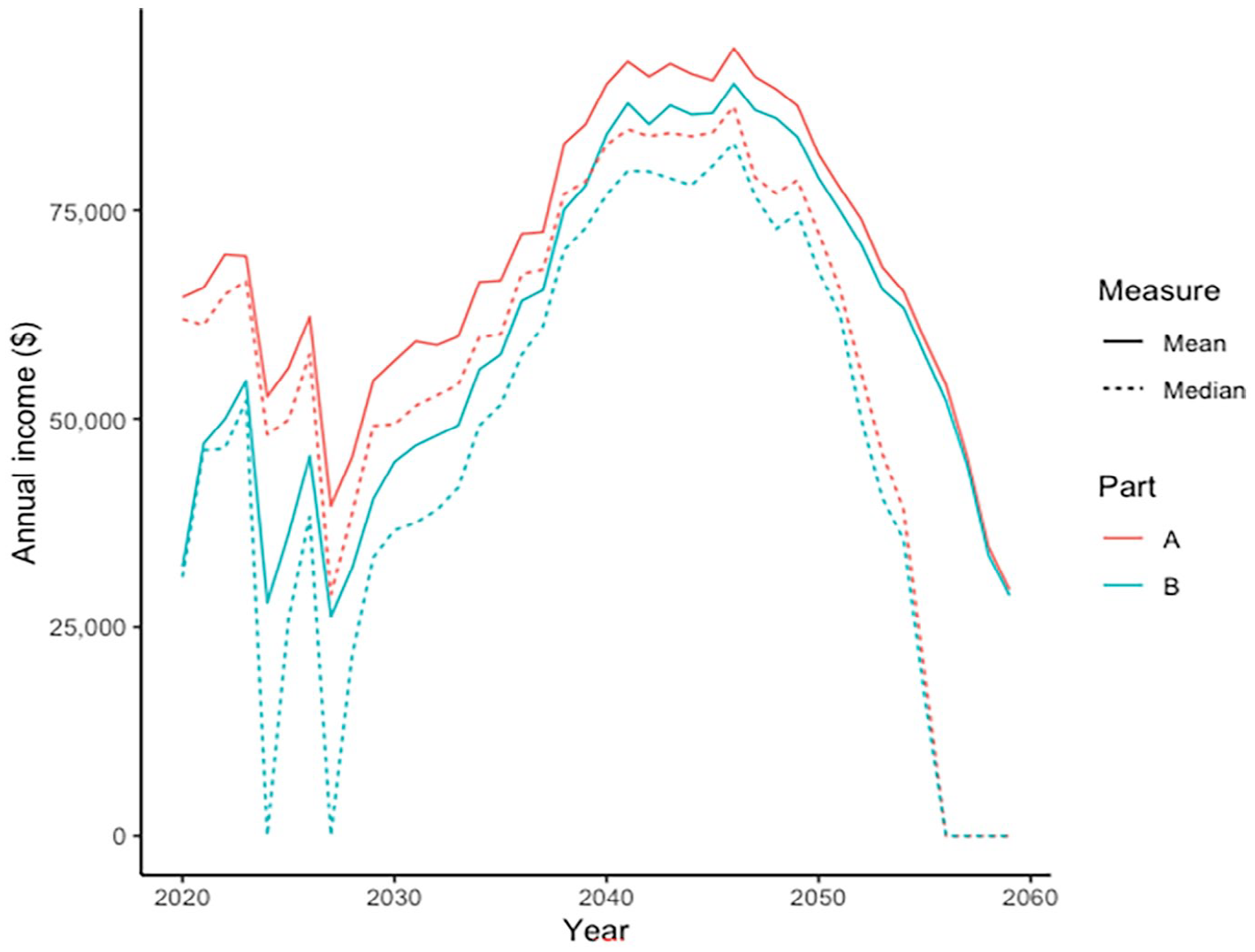
Margherita’s annual income.

4.2.2. Labour force status impact

The impact of adverse employment experiences during 2020 was dependent on various factors. This includes the type of labour force change (a reduction of hours or losing employment), the foregone salary and the time taken to return to a prior employment state, with impacts compounded over time.

Labour force resilience depended not only on the type of employment shock, but also on the propensity of being in the original state given the individual characteristics. Although past employment is a strong indicator of future employment status, other covariates are also important determinants of labour force recovery following an employment shock. This includes age, gender, education, marital status and age of children.

Given that recent employment history is influential on future labour force movement, cameos were selected such that their prior employment history was steady, to demonstrate the impact of a sudden shock, rather than a regular downturn. However, for those with young children or who had only recently entered the labour force (such as Aoife who spent 2019 out of the labour force as she gave birth to her child), a second consecutive year out of the labour force in 2020 would substantially decrease her probability of being employed for several years.

In terms of particular cameos, the labour force effect was greatest for Margherita and Johan. Both lost FT work, with the effects of lost contributions compounding over their relatively long time remaining before retirement.

Figure 2.

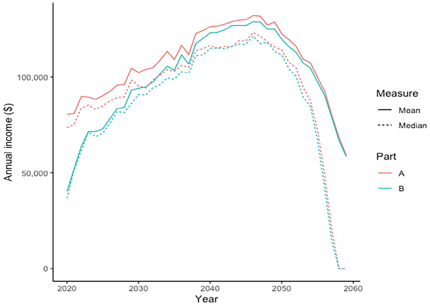
Johan’s annual income.

Figure 3.

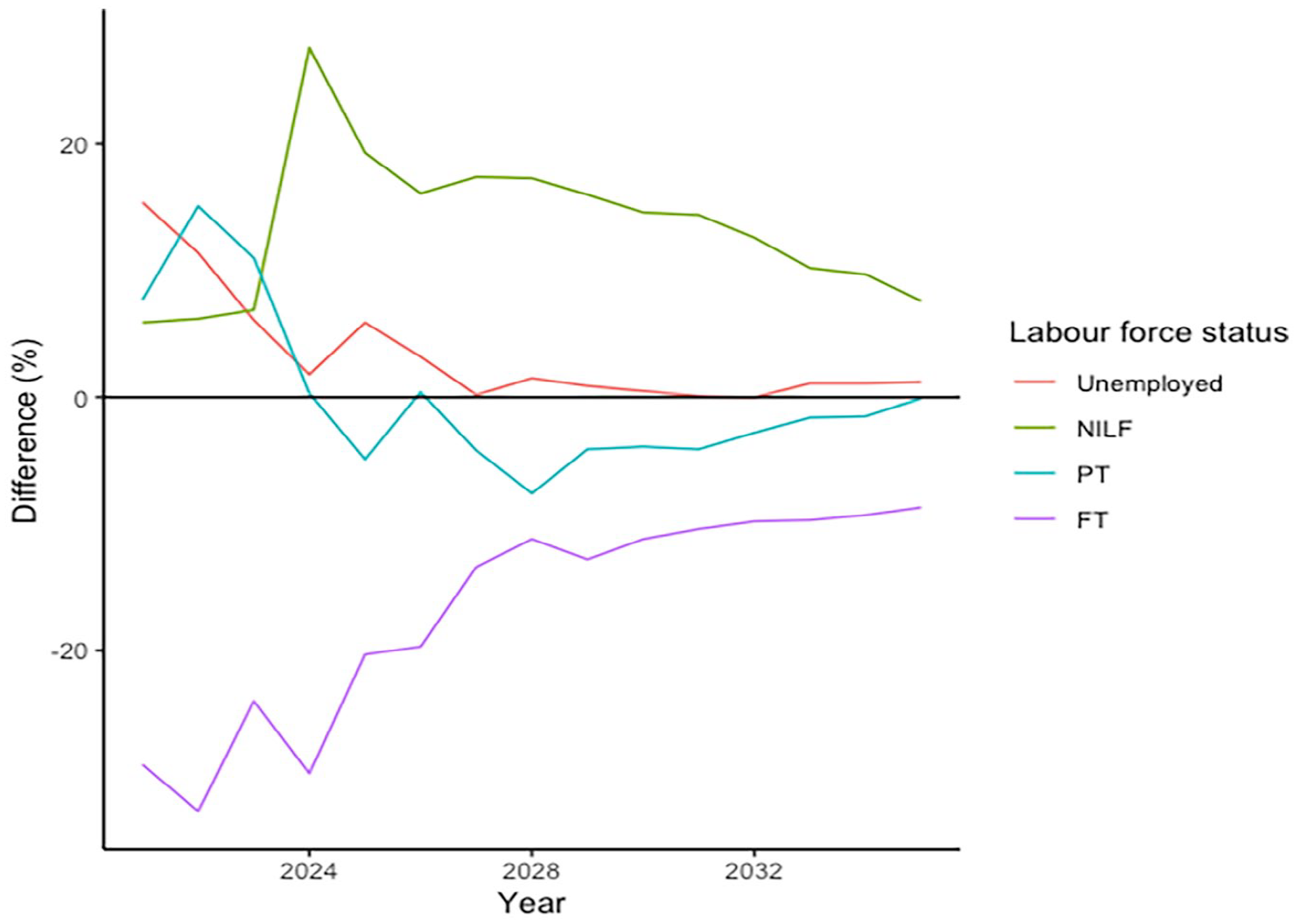
Margherita’s LF status impact.

Figure 4.

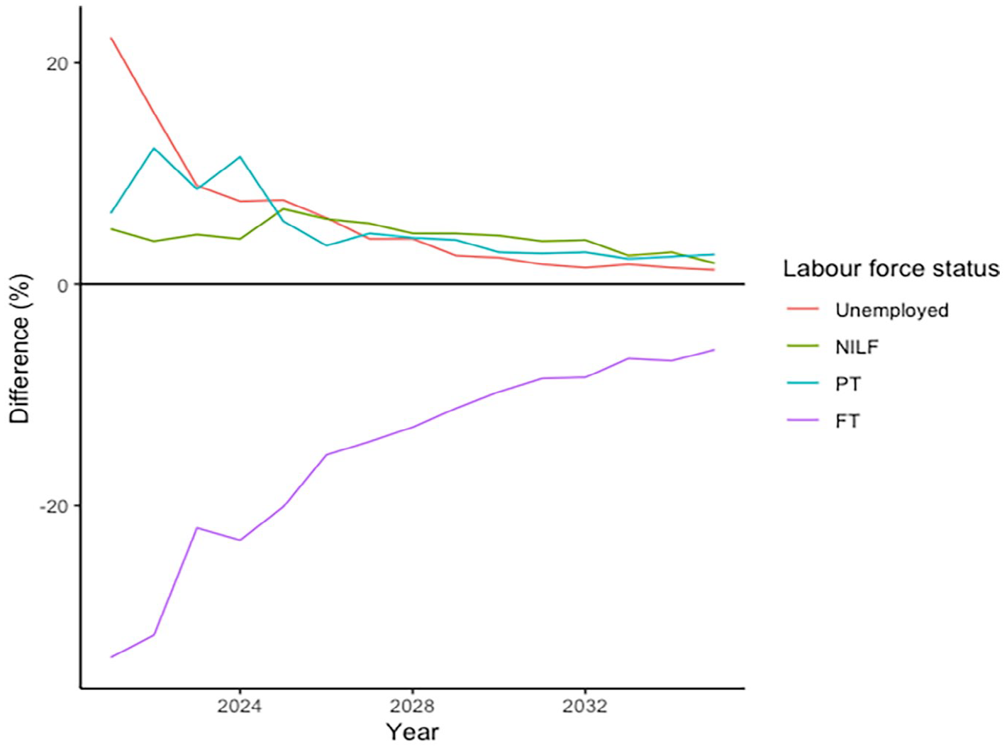
Johan’s LF status impact.

The immediate fall in Johan’s taxable income was greater than Margherita’s, but his labour force recovery was less turbulent. This is despite Johan being unemployed in 2020, meaning that his return to employment is more likely to be through PT work compared to expectations prior to COVID-19. Margherita’s period out of the workforce increased her probability of remaining out of the workforce once she had children, thereby impacting her long-term employment prospects. This speaks to COVID-19’s exacerbation of gender differences in financial matters, a point discussed in more detail shortly.

As a comparison to Johan and Margherita, the lowest impacts were for Julie and Connal, and Lucy and Laurence. For Julie and Connal, their labour force shock of losing PT work was not as large as for Margherita and Johan, their foregone income in 2020 was much lower and their employment recovery was stronger because of their qualifications and position at the start of their careers.

For Laurence and Lucy, someone with Lucy’s characteristics has a higher propensity to work PT than someone with Laurence’s characteristics, ignoring employment history. Lucy’s probability of not working also increased by more than Laurence’s as the pair approach age 60, meaning that the 2020 labour shock is more likely to bring on an earlier exit from the workforce for Lucy than Laurence.

While Laurence’s expected income in 2020 (and therefore his foregone income in 2020 when his hours worked are reduced) is higher than Lucy’s, his stronger labour force recovery meant that his median retirement balance loss is also lower than Lucy’s.

Dorris and Duncan were more impacted than Lucy and Laurence, as they lost employment rather than having a reduction in hours. Their income lost in 2020 was therefore greater and their return to full employment slower than if they kept their jobs. Being older, their propensity of full employment was lower and therefore harder to achieve than for Lucy and Laurence.

Figure 5.

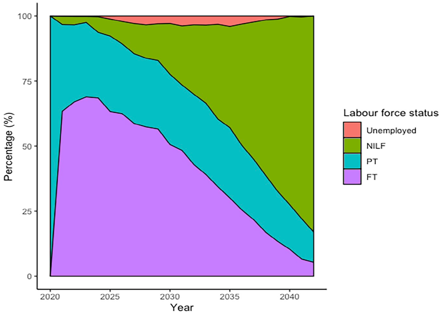
Lucy’s LF probabilities.

Figure 6.

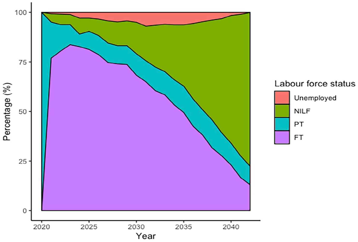
Laurence’s LF probabilities.

Figure 7.

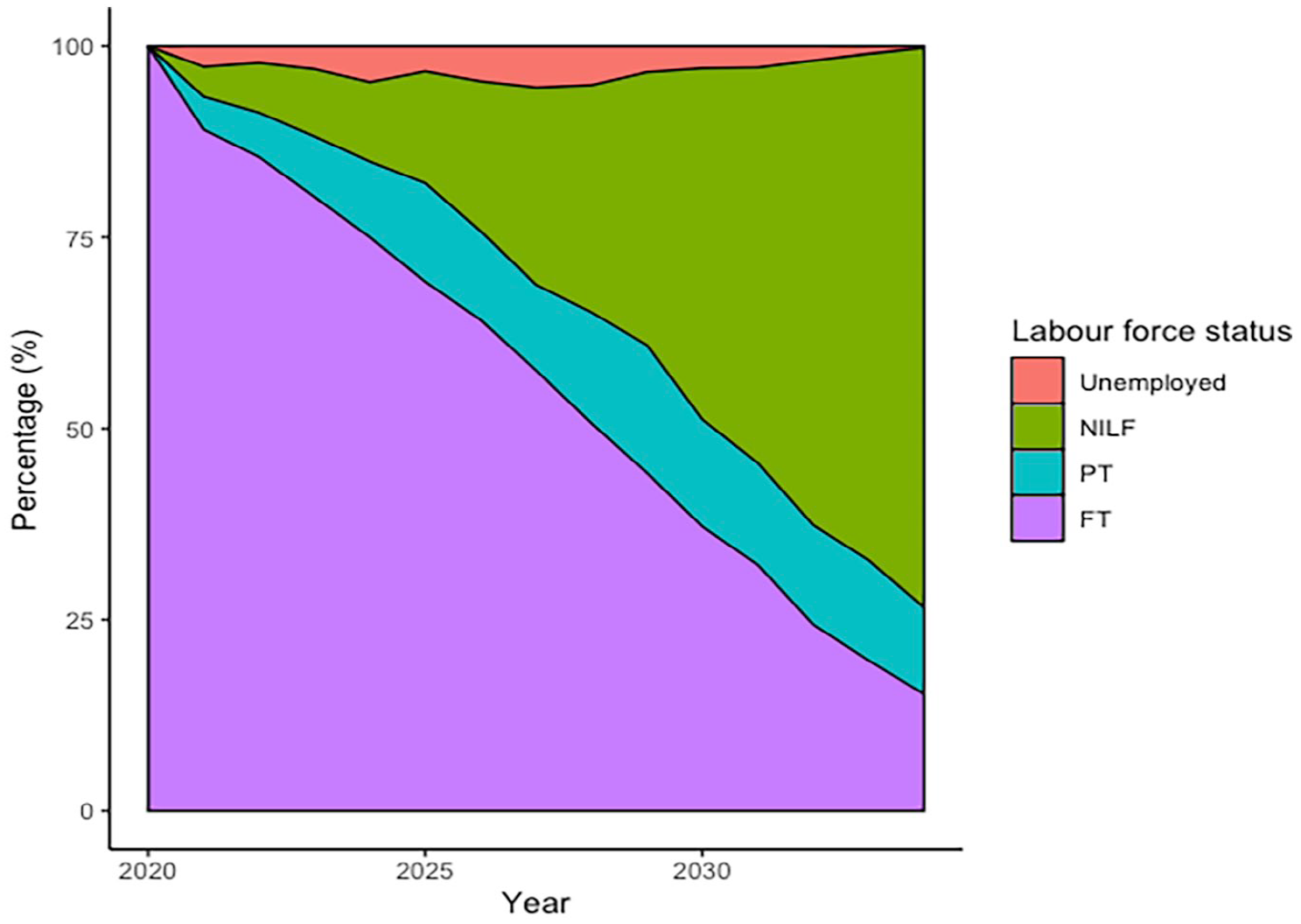
Part A – Duncan LF propensity.

Figure 8.

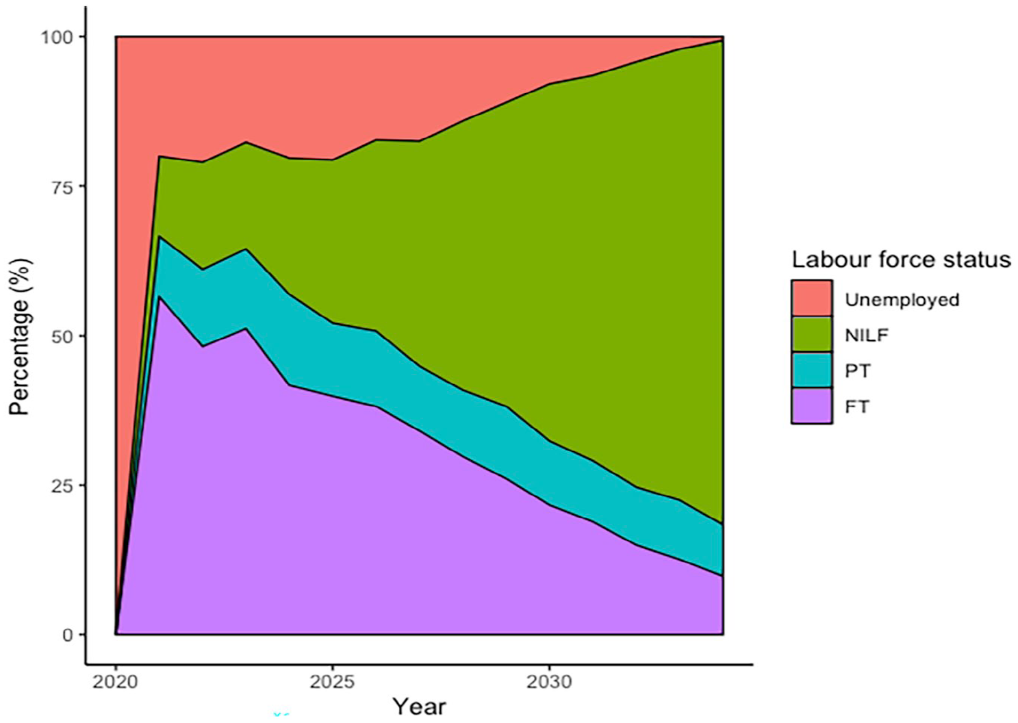
Part B – Duncan LF propensity.

Figure 9.

Impact of low wage growth on retirement balances.

4.2.3. Wage growth impact

The impact of a fall in wage growth increased with the number of years remaining in the labour force, and hence was greatest for Julie and Connal. This was due to the divergence of the Part A and Part B wage indexes series over time but also due to the effect of compounding investment returns. The absolute impact was greater for those with greater income.

4.2.4. Cash impact

Dorris and Duncan were close to retirement and had more superannuation than other cameos. Therefore, with more vulnerability to market downturns, they switched their superannuation to cash investment options to minimise further losses. As such, they missed out on the strong 2021 market recovery, with the impact effectively the difference between the market return (17.7%) and the cash return (0.25%) in the 2020–2021 financial year, and was further exacerbated by future superannuation returns over the remaining time until retirement. The cost to Duncan was higher than to Dorris given his higher starting superannuation balance.

4.2.5. Superannuation returns impact

The modelled impact of a poor investment performance for a balanced superannuation fund in the 2019–2020 financial year was small, given it was accompanied by a strong recovery in the 2020–2021 financial year. The observed 2-year return here was greater than the expected 2-year random variable return modelled. While those nearing retirement may have seemed at risk after market losses in early 2020, superannuation is a long-term investment, with a steady drawdown on assets in retirement.

4.3. Standards of living

A third mechanism to examine the impact of COVID-19 was the probability of meeting ASFA standards of living benchmarks in retirement. Results from simulation outputs are given below.

Table 6.

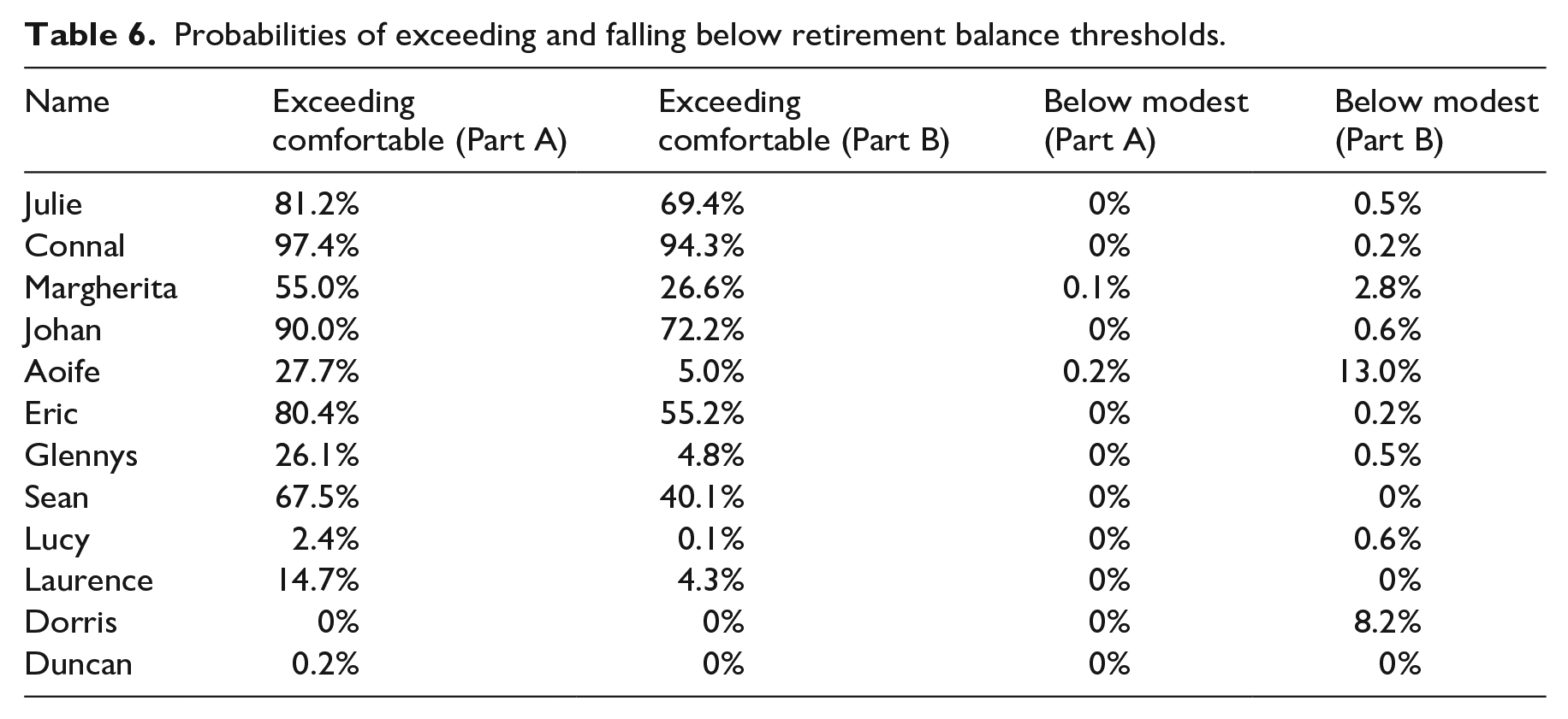
Probabilities of exceeding and falling below retirement balance thresholds.

Name	Exceeding comfortable (Part A)	Exceeding comfortable (Part B)	Below modest (Part A)	Below modest (Part B)
Julie	81.2%	69.4%	0%	0.5%
Connal	97.4%	94.3%	0%	0.2%
Margherita	55.0%	26.6%	0.1%	2.8%
Johan	90.0%	72.2%	0%	0.6%
Aoife	27.7%	5.0%	0.2%	13.0%
Eric	80.4%	55.2%	0%	0.2%
Glennys	26.1%	4.8%	0%	0.5%
Sean	67.5%	40.1%	0%	0%
Lucy	2.4%	0.1%	0%	0.6%
Laurence	14.7%	4.3%	0%	0%
Dorris	0%	0%	0%	8.2%
Duncan	0.2%	0%	0%	0%

Figure 10.

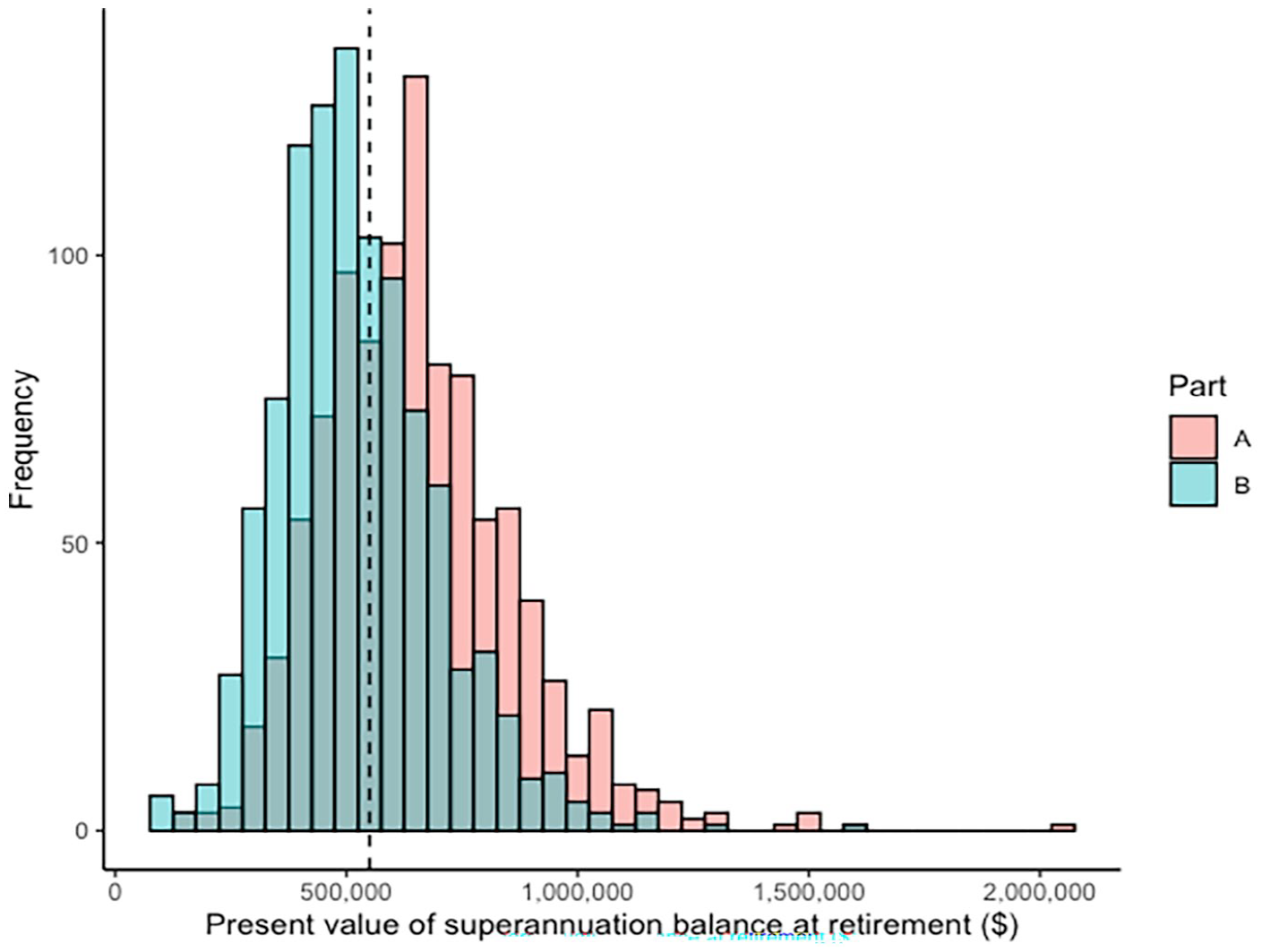
Sean retirement balance distributions, with comfortable threshold.

Given the role of the maturing superannuation system, the probability of not meeting a modest standard of living was generally low for each cameo. However, for those who lost a large proportion of their superannuation and have risks in returning to the workforce (e.g. Aoife and Dorris), the probability of not meeting the modest standard increased significantly to 13% and 8.2%, respectively. Those with higher superannuation balances had no discernible decrease in achieving a modest retirement standard.

The impact on reaching a comfortable standard of living in retirement was more significant. For example, both Sean and Margherita had projected median retirement balances above the comfortable benchmark before COVID-19, but lower than the benchmark after COVID-19. A large number of simulation outputs were concentrated around the median, hence the movement in comfortable threshold probabilities.

While Glennys and Aoife did not have a high probability of reaching this benchmark prior to COVID-19, their probabilities further reduced, to just 5%. In contrast, although Connal faced one of the largest nominal financial impacts of COVID-19, his high projected superannuation balance means that his probability was only reduced by a small amount.

For several cameos, the majority of retirement outcomes lie between the modest and comfortable standards. For example, Duncan withdrew the full ERS amount and switched his investment strategy to cash. Nearly all of his simulated superannuation balances at retirement fall between the two thresholds, and this wedge in superannuation between Part A and Part B is difficult to overcome given his proximity to retirement and the narrow distribution of his discounted future income.

Figure 11 demonstrates that the impact on Duncan is likely to be considerable. Given that his Part A distribution’s lower tail is close to the mode of his Part B distribution, this represents a tangible impact of COVID-19.

Figure 11.

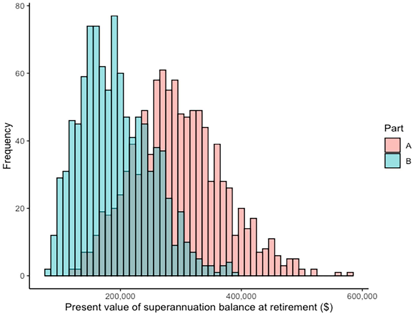
Duncan retirement balance distributions.

4.4. Interaction with age pension

Retirement income lost as a result of lower superannuation balances will be partly offset in some cameos by increases in future age pension payments. However, those with lower projected superannuation balances were more likely to be eligible for the maximum rate of age pension anyway, and therefore any losses are not supplemented by additional age pension receipts. Those with high superannuation balances at retirement may not be immediately eligible for any amount of age pension at retirement even after incurring losses. However, any superannuation losses from COVID-19 will increase the probability of future eligibility and the period of age pension receipt.

Table 7.

Gender gaps from median retirement balances.

Pair	Part A gap ($)	Part B gap ($)	Part A gap	Part B gap
Julie & Connal	386,609	324,839	32.3%	32.0%
Margherita & Johan	316,918	299,328	34.8%	43.1%
Aoife & Eric	312,879	326,400	42.2%	56.9%
Glennys & Sean	190,228	194,829	29.8%	38.4%
Lucy & Laurence	99,672	105,525	24.6%	32.1%
Dorris & Duncan	79,974	69,430	27.6%	37.1%

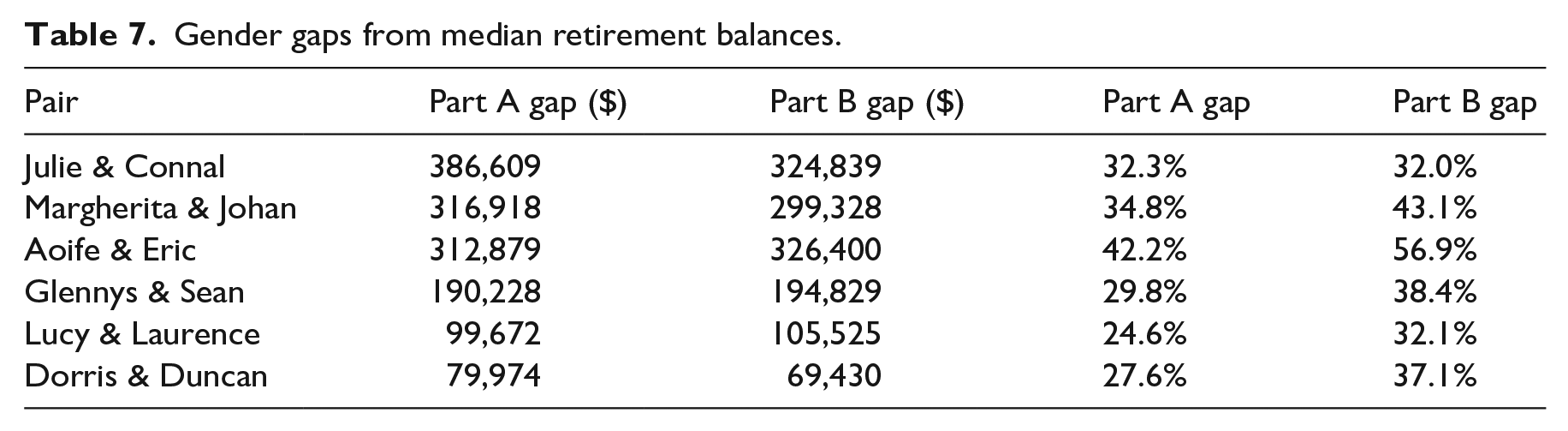
4.5. Gender gap

An approach to examine the impact on the aforementioned gender gap in superannuation savings is to consider same-aged pairs of cameos. A main driver of disparities will be differing periods out of the workforce, in addition to plateauing wages and short-term income declines. Also, identical ERS withdrawals will increase the percentage gap in superannuation if a prior gap exists.

The percentage gender gap in superannuation was increased by COVID-19 for all but one of the pairs. For each pair, the male’s starting superannuation was higher than the female’s, but their ERS amount were identical, contributing to this percentage gap. The exception is the youngest pair Julie and Connal, who are at the start of their careers, have identical attributes (other than gender) and after making ERS withdrawals have negligible superannuation balances. In addition, Connal experiences high wage growth impacts.

Taking career breaks to raise children has been cited as a significant driver of the current gender gap (The Treasury, 2020b). Therefore, Margherita and Aoife’s increased probability of being out of the labour force (from the 2020 labour force shock) increased the gender gap further. This gap in labour force recoveries can be sustained for a longer period, given the five lagged employment status predictors in the model. Similarly, the faster labour force recoveries observed by Sean and Laurence over their female counterparts saw their nominal gender gaps increase. The nominal superannuation gap existing between Dorris and Duncan reduced given Duncan switched more assets to cash; however, their relative gap in percentage terms increased.

Overall, the simulated results demonstrate that the gender gap in superannuation will continue to perpetuate in retirement income in the future if gender discrepancies in the form of wages and labour force participation exist during working years.

We reiterate that these results only reflect superannuation gaps for the cameos and are not (by design) indicative of a population-wide impact of COVID-19. The use of cameos in this manner does not reflect that women were overrepresented in highly affected industries and that the gender gap in average weekly ordinary time earnings increased during the pandemic (Australian Unions, 2020; Glennie et al., 2021; Hodgson, 2020).

4.6. Sensitivity analysis

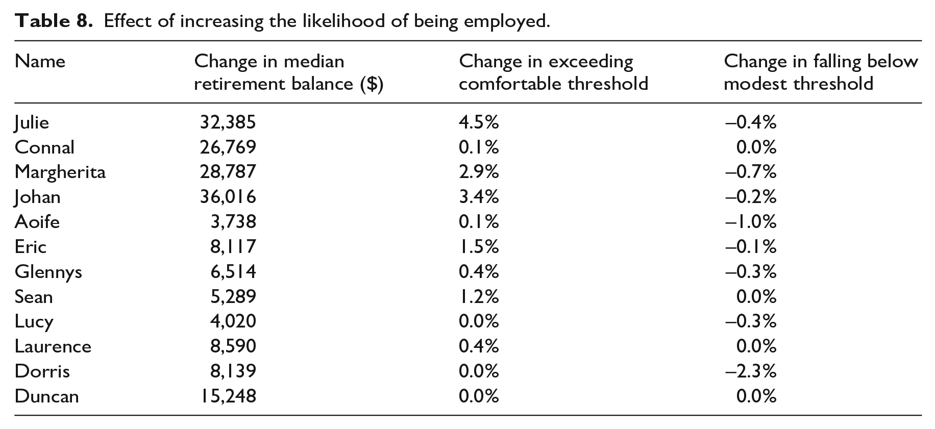
With the large labour force contraction in early 2020, there are increased uncertainties in the size of the labour market and in the impact on labour force transitions in the short to medium term. Therefore, as a form of sensitivity analysis, the probability of being employed was increased and decreased by 10% over the 2021–2022 to 2023–2024 financial years. The following gives the impact of the 10% increase.

With a higher likelihood of returning to employment, those who benefit most are those who lost employment in 2020. Younger cameos benefit more from compounding effects up to retirement, giving higher likelihoods of reaching a comfortable standard of living in retirement. For the modest threshold, Aoife and Dorris benefit most, given that their modelled labour force recoveries were not strong.

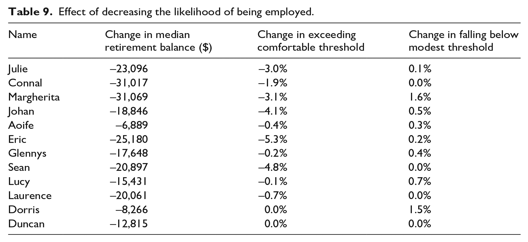
The following gives the impact of the 10% decrease.

The sensitivity of labour force probabilities on retirement superannuation balances is more concentrated for young people, given the effect of compounding investment returns. Comparing Tables 8 and 9 suggests that the downside associated with lower employment is greater than the upside of high employment, at least for these cameos. For example, the decline in exceeding the comfortable threshold at retirement was generally greater than the earlier increases. This is seen with Margherita, whose relative increase in falling below a modest threshold highlights the negative impact of an extended period of no contributions.

Table 8.

Effect of increasing the likelihood of being employed.

Name	Change in median retirement balance ($)	Change in exceeding comfortable threshold	Change in falling below modest threshold
Julie	32,385	4.5%	–0.4%
Connal	26,769	0.1%	0.0%
Margherita	28,787	2.9%	–0.7%
Johan	36,016	3.4%	–0.2%
Aoife	3,738	0.1%	–1.0%
Eric	8,117	1.5%	–0.1%
Glennys	6,514	0.4%	–0.3%
Sean	5,289	1.2%	0.0%
Lucy	4,020	0.0%	–0.3%
Laurence	8,590	0.4%	0.0%
Dorris	8,139	0.0%	–2.3%
Duncan	15,248	0.0%	0.0%

Table 9.

Effect of decreasing the likelihood of being employed.

Name	Change in median retirement balance ($)	Change in exceeding comfortable threshold	Change in falling below modest threshold
Julie	–23,096	–3.0%	0.1%
Connal	–31,017	–1.9%	0.0%
Margherita	–31,069	–3.1%	1.6%
Johan	–18,846	–4.1%	0.5%
Aoife	–6,889	–0.4%	0.3%
Eric	–25,180	–5.3%	0.2%
Glennys	–17,648	–0.2%	0.4%
Sean	–20,897	–4.8%	0.0%
Lucy	–15,431	–0.1%	0.7%
Laurence	–20,061	–0.7%	0.0%
Dorris	–8,266	0.0%	1.5%
Duncan	–12,815	0.0%	0.0%

Figure 12.

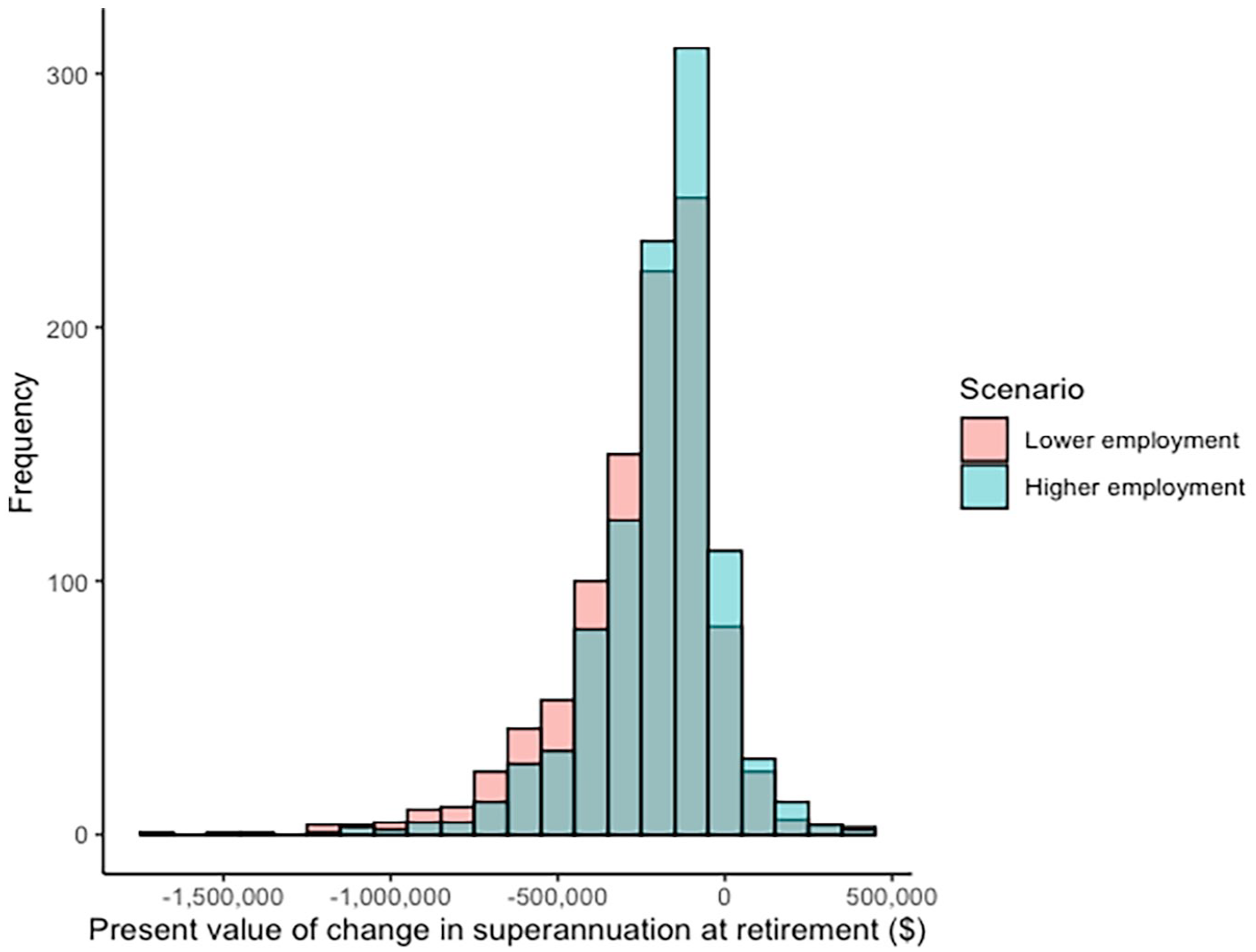
Johan Part B loss distributions under adjusted employment probabilities.

Differences in median balances is a useful metric for quantifying the impact of adjusting labour force transitions, but this does not correspond to a shift of equivalent amount in the distributions of outcomes. Simulations with high losses between Part A and Part B retirement balances were likely absorbed in unemployed or NILF states for an extended period of time, as a result of the imposed 2020 labour shock. Given the fitted lagged employment covariates in the labour force transition model, the probability of returning to employment decreases for each successive year out of the workforce. By increasing the likelihood of being out of the workforce until 2023, the probability of experiencing an extended period out of the workforce increases and therefore the distribution of losses between Part A and Part B becomes more negatively skewed. This is illustrated below.

Here, the skewness of losses under increased probability of employment is −1.16, compared to −1.41 under a scenario of decreased probability of employment, indicating a higher level of negative skewness under this latter scenario.

5. Discussion

The ERS scheme provided timely liquidity to Australians in a climate of high economic uncertainty. Take-up of the scheme was high, and as the sums released were self-funded, it can be framed as an effective fiscal measure in the short term. While standard government unemployment benefits may potentially discourage labour force participation, the ERS scheme did not introduce any obvious, similar moral hazard (Gerards and Welters, 2020). In addition, the scheme served as an economic stimulus, providing funds to a self-selected group that either identified that their immediate needs were greater than their future requirements or did not consider such trade-offs in an explicit manner.

However, the value of an ERS withdrawal accumulated to retirement can be significant, particularly for younger ERS recipients. For cameos that remained employed, an ERS withdrawal was the major contributor to a reduced projected retirement balance. That said, for most of the cameos modelled, the probability of falling below a modest standard of living in retirement did not increase significantly by electing to withdraw.

The ERS also facilitated the sale of superannuation assets at their lowest point after the market shock, foregoing later market recovery (Wherrett et al., 2021) and posing additional liquidity challenges for the superannuation industry, particularly for a small number of industry funds with young members (HESTA, 2020). It poses an interesting case study for future liquidity stress testing, which may need to capture the simultaneous aggregation of fund withdrawals, member switching and market downturns. The release of Prudential Standard SPS530 (APRA, 2023) itself partly reflects insights from COVID-19’s impact on stress testing and liquidity management (Alleston, 2023).

The impacts of COVID-19 on retirement are not isolated to those who withdrew ERS in 2020. The cameos indicate that while younger individuals are exposed to greater nominal costs by retirement due to the effect of compounding returns, older Australians are also highly vulnerable, especially those who do not own their own home.

How to restore or adapt to lower superannuation balances at retirement is an open question. Delaying retirement to spend a longer time in the workforce is an obvious response, to increase savings and decrease the number of years for which retirement savings are needed. However, participating in the labour force for longer may not be feasible for many and the benefits of retiring later may be limited, given the expected hourly wage for those at this age is relatively low. Increasing voluntary contributions is an option, but this also depends on sustained employment and other issues such as cost of living pressures. Furthermore, to assist those who withdrew ERS amounts, the government legislated a measure in July 2021 to allow re-contributions to superannuation, without these amounts counting towards non-concessional caps, if completed before 30 June 2030 (Treasury Laws Amendment Act, 2021, sch 3). It remains to be seen how many Australians that accessed superannuation during financial distress are in a position over the next several years to respond to this legislation.

There is also a wider question around behavioural adaptation. Are people concerned enough about an impact on a future level of savings, when more pressing concerns are high living costs and challenges in home affordability? This is especially relevant for the younger cohorts, where the full impact on superannuation emerges over a long period of time and becomes subsumed by a new ‘normal’ in terms of expectation and mental framing over that same long period of time.

To a degree, COVID-19 has increased the level of individual responsibility for retirement well-being. As such, an ongoing challenge is generating individual engagement in financial choices, particularly for those who can understandably struggle with the complexity of the superannuation system as well as uncertainty (Bruhn, 2019; Cheah et al., 2015; Levy, 2023). This highlights the relevance and importance of an effective and accessible financial advice industry, which has its own challenges (Bruhn and Asher, 2021; Bruhn and Miller, 2014). It also highlights key roles that superannuation funds can themselves play in education, engagement, access to advice and development of effective products. This could include, for example, personalised communications to members who have withdrawn (Wang-Ly and Newell, 2022). For similar responses to future crises, it could also include clear information around the long-term consequences of withdrawing, or other safeguards such as more personalised limits in withdrawal amounts (Bateman et al., 2023; Wang-Ly and Newell, 2022).

6. Conclusion

The economic impact of COVID-19 has been significant. This included impacts on the superannuation savings of many Australian, which has a critical role for financial provision in retirement. As such, the projected impact of COVID-19 on superannuation balances at retirement was assessed for 12 cameos. A heterogeneity in impacts across these cameos is evident. For ERS participants, the associated reduction in superannuation balances will compound over time to retirement. For young recipients who are decades away from complete access to their superannuation, this compounding affect is significant. However, this cohort is also more likely to enjoy a greater proportion of their careers with higher rates of superannuation contributions than older Australians, resulting in higher likelihoods of achieving adequacy in retirement. Conversely, those closer to retirement with low superannuation balances face a reduced probability of reaching either a comfortable or modest standard of retirement income. This cohort would have already been likely to qualify for the full-rate age pension, meaning this loss in superannuation will not be supplemented by increased marginal age pension income. Those with less resilience to a labour force shock are projected to have significantly reduced superannuation assets at retirement.

In terms of model limitations and improvements, a more sophisticated framework such as a Wilkie investment model could be used to incorporate the association between inflation, wage growth and investment returns. Furthermore, the employment regression estimates are unlikely to represent transition probabilities in the long term, 45 years into the future. Future modelling could incorporate improvement factors to employment status probabilities for particular cohorts for later forecast years. Sampling HILDA surveys without replacement and including covariates to proxy the point in time as well as the economic climate, may be one way to build a labour force status transition model.

The hours worked component of the model was relatively simplistic, and further determinants of hours worked could be established for more meaningful distributions. Hours worked could be incorporated as a covariate to employment state transition probabilities, where someone working PT transitioning to FT would increase with their PT hours worked. Reductions in hours worked could be explicitly modelled rather than shifts in employment states.

In terms of scope, this article has not examined the opportunity cost of not using ERS withdrawals. Access to the ERS provided timely assistance for many participants, and the counterfactual of what their situation would have been without ERS is unknown. Might more financial assistance from wider family networks have been forthcoming, or would the use of predatory lenders become more prevalent, together with its obvious consequent risks?

One extension of this work is to consider the situations of couples, rather than just individuals. A rudimentary approach could be to pair same-age cameos together, including their superannuation at retirement. However, this would require development of the dependencies between the combined financial position with future labour force participation, among other things. Finally, the simulation model could be applied to all individuals who accessed ERS, if the data were available, to quantify the collective or cohort-specific impacts.

Footnotes

Acknowledgements

The authors acknowledge the comments and support provided by Dr Bronwyn Loong, Dr Jananie William and Dr Tim Higgins at the Research School of Finance, Actuarial Studies and Statistics, Australian National University.

Final transcript accepted 8 August 2024 by Tom Smith (AE Finance).

Funding

The author(s) disclosed receipt of the following financial support for the research, authorship, and/or publication of this article: The authors thank the Australian National University for the facilities and resources to enable this research to occur.

ORCID iD

Aaron Bruhn

1.

Australian Super, Aware Super, REST, CBUS, SunSuper, QSuper, HESTA, HOSTPLUS, Unisuper, sourced by APRA quarterly MySuper statistics.

References

ABC News (2020) Coronavirus COVID-19 pandemic phase will call for ‘extreme measures’, Victorian Premier Daniel Andrew says. Available at: https://www.abc.net.au/news/2020-03-10/victorian-premier-daniel-andrews-on-coronavirus-pandemic-plans/12042780 (accessed 12 September 2021).

ABS (2020a) Wage Price Index, Australia. Available at: https://www.abs.gov.au/statistics/economy/price-indexes-and-inflation/wage-price-index-australia/jun-2020#spotlight-wage-reductions (accessed 30 June 2021).

ABS (2020b) Wage Price Index, Australia. Available at: https://www.abs.gov.au/statistics/economy/price-indexes-and-inflation/wage-price-index-australia/sep-2020 (accessed 30 June 2021).

ABS (2020c) Wage Price Index, Australia. Available at: https://www.abs.gov.au/statistics/economy/price-indexes-and-inflation/wage-price-index-australia/dec-2020 (accessed 30 June 2021).

ABS (2020d) Australian National Accounts: National income, expenditure and product. Available at: https://www.abs.gov.au/statistics/economy/national-accounts/australian-national-accounts-national-income-expenditure-and-product/jun-2020 (accessed 22 September 2021).

ABS (2020e) Household financial resources. Available at: https://www.abs.gov.au/statistics/economy/finance/household-financial-resources/sep-2020 (accessed 27 September 2021).

ABS (2021a) One year of COVID-19: Aussie jobs, businesses and the economy. Available at: https://www.abs.gov.au/articles/one-year-covid-19-aussie-jobs-business-and-economy (accessed 12 June 2021).

ABS (2021b) Labour force, Australia. Available at: https://www.abs.gov.au/statistics/labour/employment-and-unemployment/labour-force-australia/latest-release (accessed 26 June 2021).

ABS (2021c) Wage Price Index. Australia. Available at: https://www.abs.gov.au/statistics/economy/price-indexes-and-inflation/wage-price-index-australia/jun-2021 (accessed 19 August 2021).

10.

ABS (2021d) Australian National Accounts: National income, expenditure and product. Available at: https://www.abs.gov.au/statistics/economy/national-accounts/australian-national-accounts-national-income-expenditure-and-product/latest-release (accessed 27 September 2021).

11.

Alleston (2023) How super funds are bolstering trust in their valuations. Available at: https://www.spglobal.com/marketintelligence/en/mi/research-analysis/how-super-funds-are-bolstering-trust-in-their-valuations.html (accessed 15 January 2024).

12.

Andrews

Deutscher

Hambur

, et al. (2019) Wage growth in Australia: Lessons from longitudinal microdata. Available at: https://treasury.gov.au/sites/default/files/2019-07/2019-04_wage_growth_in_australia_lessons_from_longitudinal_microdata.pdf (accessed 14 August 2021).

13.

APRA (2021) COVID-19 early release scheme – Issue 36. Available at: https://www.apra.gov.au/covid-19-early-release-scheme-issue-36 (accessed 7 February 2021).

14.

APRA (2023) Prudential standard SPS 530 – investment governance. Available at: https://www.apra.gov.au/sites/default/files/2022-07/Prudential%20Standard%20SPS%20530%20Investment%20Governance.pdf (accessed 15 January 2024).

15.

ASFA (2018) ASFA retirement standard. Available at: https://www.superannuation.asn.au/ArticleDocuments/269/2109-ASFA-Retirement_Standard_Summary.pdf (accessed 18 April 2021).

16.

ASFA (2020a) Superannuation statistics June 2020. Available at: https://www.superannuation.asn.au/ArticleDocuments/269/SuperStats-Jun2020.pdf (accessed 22 September 2021).

17.

ASFA (2020b) Experience to date with the early release of superannuation. Available at: https://www.superannuation.asn.au/wp-content/uploads/2023/09/2006-Experience-to-date-with-the-early-release-of-superannuation.pdf (accessed 26 June 2021).

18.

ASFA (2021) ASFA Economic Snapshot: Week ending 16 April. Available at: https://www.superannuation.asn.au/resources/economic-snapshot?PagingModule=8265&retain=true&Pg=3 (accessed 12 September 2021).

19.

ATO (2021) COVID-19 early release of super report (20 April-31 December 2020). Available at: https://www.ato.gov.au/about-ato/research-and-statistics/in-detail/super-statistics/early-release/covid-19-early-release-of-super (accessed 6 April 2021).

20.

ATO (2023a) When you can access your super early. Available at: https://www.ato.gov.au/individuals/super/withdrawing-and-using-your-super/early-access-to-super/when-you-can-access-your-super-early/ (accessed 22 September 2023).

21.

ATO (2023b) First home super saver scheme. Available at: https://www.ato.gov.au/individuals/super/withdrawing-and-using-your-super/first-home-super-saver-scheme/ (accessed 22 September 2023).

22.

Australian Unions (2020) Leaving women behind: The real cost of the Covid recovery. Available at: https://www.actu.org.au/media/1449315/d56-leavingwomenbehind_realcostofcovidrecovery.pdf (accessed 12 June 2021).

23.

Baker

Daniel

(2020) Rental insights: A COVID-19 collection, the Australian housing and urban research institute limited. Melbourne, VIC, Australia. https://www.ahuri.edu.au/sites/default/files/migration/documents/Rental-Insights-A-COVID-19-Collection.pdf

24.

Bateman

Dobrescu

Liu

, et al. (2023) Determinants of early access to retirement savings: Lessons from the COVID-19 pandemic. The Journal of the Economics of Ageing 24: 100441.

25.

Britton

Dearden

van der Erve

, et al. (2020) The impact of undergraduate degrees on lifetime earnings. Research report, no. DFE-RR974, Department of Education, Manchester. Available at: https://www.gov.uk/government/publications/undergraduate-degrees-lifetime-labour-market-returns (accessed 20 September 2021).

26.

Britton

van der Erve

Higgins

(2019) Income contingent student loan design: Lessons from around the world. Economics of Education Review 71: 65–82.

27.

Bruhn

(2015) Personal and social impacts of significant financial loss. Australian Journal of Management 40: 459–477.

28.

Bruhn

(2019) Relying on the heuristic of trust: A case study. Accounting & Finance 59: 333–357.

29.

Bruhn

Asher

(2021) The primacy of ethics in the provision of financial advice. Accounting & Finance 61: 3305–3327.

30.

Bruhn

Miller

(2014) Lessons about best interests duty. Australasian Accounting, Business and Finance Journal 8: 23–44.

31.

Butt

Khemka

Warren

(2022) Heterogeneity in optimal investment and drawdown strategies in retirement. Pacific-basin Finance Journal 74: 1–20.

32.

Cheah

Foster

Heaney

, et al. (2015) Discussions on long-term financial choice. Australian Journal of Management 40: 414–434.

33.

Dawson

Casey

(2020) The ‘Herstory’ of Superannuation. Per Capita. Available at: https://percapita.org.au/wp-content/uploads/2020/08/The-Herstory-of-Superannuation-FINAL-1.pdf (accessed 4 September 2021).

34.

Department of Health (2021) What you need to know about Coronavirus (COVID-19). Available at: https://www.health.gov.au/news/health-alerts/novel-coronavirus-2019-ncov-health-alert/ongoing-support-during-coronavirus-covid-19/what-you-need-to-know-about-coronavirus-covid-19 (accessed 12 September 2021).

35.

Gerards

Welters

(2020) Liquidity constraints, unemployed job search and labour market outcomes. Oxford Bulletin of Economics and Statistics 82: 625–646.

36.

Gerrans

(2012) Retirement savings investment choices in response to the global financial crisis: Australian evidence. Australian Journal of Management 37: 415–439.

37.

Glennie

von Reibnitz

William

, et al. (2021) Gender Pay Gap Reporting in Australia – Time for an Upgrade. Canberra, ACT, Australia: The Australian National University.

38.

Haynes

Western

, et al. (2006) Methods for categorical longitudinal survey data: Understanding employment status of Australian Women. In: Paper presented to the methods for longitudinal surveys conference, University of Essex, Colchester, 12–14 July 2006. Available at: https://melbourneinstitute.unimelb.edu.au/assets/documents/hilda-bibliography/conference-papers-lectures/2006/Haynes_Western_Evaluation_of_Methods_MOLS.pdf (accessed 6 August 2021).

39.

HESTA (2020) Early release super scheme sees younger women drain super. Media Release. Available at: https://www.first5000.com.au/blog/early-release-super-scheme-sees-younger-women-drain-super/ (accessed 27 August 2021).

40.

Higgins

(2011) Implications of earnings model complexity to costing income contingent loans. Unpublished Working Paper. Available at: https://papers.ssrn.com/sol3/papers.cfm?abstract_id=1810134 (accessed 18 April 2021).

41.

Higgins

Sinning

(2013) Modeling income dynamics for public policy design: An application to income contingent student loans. Economics of Education Review 37: 273–285.

42.

Hodgson

(2020) Superannuation and Covid-19: What does early access mean for women? The Power to Persuade. Available at: http://www.powertopersuade.org.au/blog/superannuation-and-covid-19-what-does-early-access-mean-for-women/17/4/2020 (accessed 18 April 2021)

43.

Industry Super Australia (2020) Super wipe out: Almost 500,000 Australians have emptied their nest eggs. Available at: https://www.industrysuper.com/assets/FileDownloadCTA/MR_Super-Wipe-Out-Almost-500000-Australians-have-emptied-nest-eggs_2-July-2020.pdf (accessed 4 September 2021).

44.

Kalb

Meekes

(2020) Wage growth distribution and changes over time: 2001-2018. Melbourne Institute Working Paper. Available at: https://melbourneinstitute.unimelb.edu.au/__data/assets/pdf_file/0008/3386762/wp2020n08.pdf (accessed 15 August 2021).

45.

Knox

Rice

Dunn

(2021) Gender inequality in retirement savings. Actuaries Institute. Available at: https://www.actuaries.asn.au/Library/Miscellaneous/2021/GenderInequalityinRetirementSavingsActuariesInstitute270421.pdf (accessed 30 April 2021).

46.

Lamarra

Bruhn

Miller

, et al. (2022) Stochastic modelling of the home equity access scheme. Australian Journal of Management 48: 652–677.

47.

Levy

(2023) Quality of advice review – final report, Australian Treasury. Available at: https://treasury.gov.au/publication/p2023-358632 (accessed 17 January 2024).

48.

Lin

Bruhn

William

(2019) Extending financial literacy to insurance literacy: A survey approach. Accounting & Finance 59: 685–713.

49.

McIlroy

(2022) Super early access delayed unemployed returning to work, Australian Financial Review. Available at: https://www.afr.com/politics/federal/super-early-access-delayed-unemployed-returning-to-work-20220915-p5bi9y (accessed 10 October 2022).

50.

Mercer (2020) Mercer CFA Institute Global Pension Index. Melbourne, VIC, Australia: Mercer.

51.

Prime Minister of Australia (2020) Supporting Australian workers and business. Media Release. Available at: https://www.pm.gov.au/media/supporting-australian-workers-and-business (accessed 12 September 2021).

52.

RBA (2020a) Statement by Philip Lowe, Governor: Monetary policy decision. 2020-06. Available at: https://www.rba.gov.au/media-releases/2020/mr-20-06.html (accessed 29 June 2021).

53.

RBA (2020b) Statement by Philip Lowe, Governor: Monetary policy decision. 2020-08. Available at: https://www.rba.gov.au/media-releases/2020/mr-20-08.html (accessed 29 June 2021).

54.

RBA (2021a) Financial Stability Review. Available at: https://www.rba.gov.au/publications/fsr/2021/apr/pdf/financial-stability-review-2021-04.pdf (accessed 27 August 2021).

55.

RBA (2021b) Recession. Available at: https://www.rba.gov.au/education/resources/explainers/recession.html (accessed 22 September 2021).

56.

Robertson

(2020) Super funds have been battered by Coronavirus, but panic is your worst enemy. ABC News. Available at: https://www.abc.net.au/news/2020-05-22/superannuation-during-covid-19-do-not-panic/12273076 (accessed 30 June 2021).

57.

Salt

(2021) Rethinking retirement: The impact of demographic change and the pandemic on retirement planning in the 2020S. ASFA. Available at: https://www.superannuation.asn.au/wp-content/uploads/2023/09/2102-Rethinking-retirement.pdf (accessed 26 June 2021).

58.

Storen

Corrigan

(2020) COVID-19: A chronology of state and territory government announcements (Up until 30 June 2020). Commonwealth of Australia. Available at: https://parlinfo.aph.gov.au/parlInfo/download/library/prspub/7614514/upload_binary/7614514.pdf (accessed 12 September 2021).

59.

The Treasury (2017) Analysis of wage growth. Commonwealth of Australia. Available at: https://treasury.gov.au/sites/default/files/2019-03/p2017-t237966.pdf (accessed 14 August 2021).

60.

The Treasury (2020a) Early access to superannuation. Australian Government. Available at: https://treasury.gov.au/sites/default/files/2020-07/Fact_sheet-Early_Access_to_Super.pdf (accessed 22 September 2021).

61.

The Treasury (2020b) Retirement income review. Commonwealth of Australia. Available at: https://treasury.gov.au/sites/default/files/2021-02/p2020-100554-udcomplete-report.pdf (accessed 11 February 2021).

62.

Treasury Laws Amendment Act (2021) Treasury Laws Amendment (More Flexible Superannuation) Act 2021 (Cth) sch 3. Available at: https://www.legislation.gov.au/Details/C2021A00045

63.

Wang-Ly

Newell

(2022) Allowing early access to retirement savings: Lessons from Australia. Economic Analysis and Policy 75: 716–733.

64.

Warren

(2021) Families in Australia Survey: Towards COVID Normal Report No. 6: The COVID-19 Early Release of Superannuation. Melbourne, VIC, Australia: Australian Institute of Family Studies.

65.

Wherrett

Cavanough

Buckland

(2021) Buy high, sell low? The early super access scheme and foregone returns on investment. The McKell Institute. Available at: https://mckellinstitute.org.au/research/articles/buy-high-sell-low-the-early-super-access-scheme-and-foregone-returns-on-investment/ (accessed 24 May 2021).

66.

World Health Organization (2020a) Novel Coronavirus (2019-nCoV) Situation report – 1. Available at: https://www.who.int/docs/default-source/coronaviruse/situation-reports/20200121-sitrep-1-2019-ncov.pdf?sfvrsn=20a99c10_4 (accessed 12 September 2021).

67.

World Health Organization (2020b) Novel Coronavirus (2019-nCoV) Situation report – 11. Available at: https://www.who.int/docs/default-source/coronaviruse/situation-reports/20200131-sitrep-11-ncov.pdf?sfvrsn=de7c0f7_4 (accessed 12 September 2021).

68.

World Health Organization (2020c) Coronavirus disease 2019 (COVID-19) Situation report – 51. Available at: https://www.who.int/docs/default-source/coronaviruse/situation-reports/20200311-sitrep-51-covid-19.pdf?sfvrsn=1ba62e57_10 (accessed 12 September 2021).

The impact of COVID-19 and the ERS on superannuation savings in Australia

Abstract

Keywords

1. Introduction

2. Background

2.1. Superannuation and retirement

2.2. COVID-19 and economic impacts

2.3. Superannuation impacts and the ERS

3. Methodology and data

3.1. Data sources

3.2. Modelling approach

3.2.1. Labour force transitions

3.2.2. Hourly wage

3.2.3. Hours worked per week

3.2.4. Wage growth

3.2.5. Superannuation returns and fees

3.3. Cameo selection

4. Results

4.1. Superannuation at retirement

4.2. Analysis of change

4.2.1. ERS impact

4.2.2. Labour force status impact

4.2.3. Wage growth impact

4.2.4. Cash impact

4.2.5. Superannuation returns impact

4.3. Standards of living

4.4. Interaction with age pension

4.5. Gender gap

4.6. Sensitivity analysis

5. Discussion

6. Conclusion

Footnotes

Acknowledgements

Funding

ORCID iD

1.

References